 Hao Guan
 Saira Hameed
 Sadaf3
 Jana Shafi
- 1Institute of Computing Science and Technology, Guangzhou University, Guangzhou, China
- 2Institute of Computer Science of Information Technology, Qiannan Normal University for Nationalities, Duyun, China
- 3Department of Mathematics, University of the Punjab, Lahore, Pakistan
- 4University of Technology and Applied Sciences, Musanna, Oman
- 5Department of Computer Engineering and Information, College of Engineering in Wadi Alddawasir, Prince Sattam Bin Abdul Aziz University, Wadi Alddawasir, Saudi Arabia
In this modern era, graph theory has become an integral part of science and technology. It has enormous applications in handling various design-based problems. In this study, we present a new approach that increases the ability of graph theory to deal with uncertain challenges. The spherical fuzzy graph addresses the uncertainty domain more broadly, going beyond classical fuzzy graphs other than generalized fuzzy graph types. The concept of the spherical fuzzy planarity value provides a new method to evaluate the edge intersection and order in the graph. The ability of the spherical fuzzy planar graph
1 Introduction
One of the most advanced fields of science is “graph theory,” which plays a vital role in the applications of other branches of science like chemistry, biology, physics, electrical engineering, computer science, discrete mathematics, astronomy, and operations research. Graph theory research has experienced significant advancements recently due to its diverse range of applications. It is also helpful in image segmentation, networking, data mining, structuring, organizing, communication, etc. For instance, a data set can be represented graphically in the form of a model, like a tree containing vertices and edges. Similarly, the concept of a graph can be used to organize network design. In many different types of graph structure applications, including design problems for electrical transmission lines, utility lines, subways, circuits, and trains, crossing through edges can be problematic. It is actually essential to run paths of communication at different levels for it to cross them. Although the positioning of the electrical cables is not extremely difficult, the cost of some types of lines can increase if subway tunnels are constructed beneath them. Specifically, circuits with a few layers in their structure are simpler to produce. Planar graphs become a framework for these applications. All the abovementioned applications utilize the concept of planar graphs. Crossing has certain benefits, such as saving space and being affordable, but it also has some disadvantages. In city road planning, due to crossing, there are increased chances of accidents because of the increasing rush of vehicles day by day. Moreover, the expenditure on crossing routes underground is high, but traffic jams are reduced on underground routes. In urban planning, it would be protective for human lives not to cross the routes. However, due to a lack of space, such crossing of routes is permitted. Generally, we use such linguistic terms as “congested, “very congested,” and “high congested”. The word congested has no definite meaning. All the abovementioned terms have some membership degrees. The choice of navigating between a congested road and a non-congested one is more favorable than navigating between two congested routes. In a fuzzy planar graph, the “congested” edges would represent strong connections between vertices, possibly indicating a high level of interaction or influence, while the “low congested” edges would represent weaker connections, perhaps suggesting a lower level of interaction or influence.
These days, science and technology deal with complicated models for which appropriate data are limited. To deal with such a phenomenon, we use mathematical models to tackle different kinds of systems that contain elements of uncertainty and vagueness. The generalization of the ordinary set theory, namely, fuzzy sets, is the foundation for handling such types of models. The concept of the fuzzy set, introduced by Lotif A. Zadeh [1] in 1965, revolutionized how we handle ambiguity and partial data in various fields. Numerous implications for fuzzy sets extend the range of investigation areas across various educational fields. In 1983, Atanassov presented the idea of an intuitionistic fuzzy set
However, aspects such as being young, smart, tall, short, healthy, and successful in a certain field cannot be easily quantified. It is possible to express these qualitative and vague predicates by defining appropriate boundaries. To enlarge the space for uncertain and vague information, Gundogdu and Kahraman [5] expanded the concept of
Based on Zadeh’s fuzzy relation [8], Kaufmann [9] introduced the concept of fuzzy graphs in 1973. Then, in fuzzy graphs, various graph-based theoretical concepts were initiated by Rosenfeld [10]. In his study of fuzzy graphs, Bhattacharya [11] made lots of remarkable perspectives about how they differ from classical graph theory. He proved that not all ideas in the field of fuzzy graphs have a direct equivalent or parallel in classical graph theory. In Mordeson and Nair [12], the idea of the complement of a fuzzy graph was introduced. A few operations on fuzzy graphs were also presented. Subsequently, the original fuzzy graph was redefined as the complement of the complement, following this change in the definition of complement. Nagoorgani and Malarvizhi [13] introduced the notion of isomorphism on fuzzy graphs. One of the most important tools of graphing is its dual graph. Abdul-Jabbar et al. [14] introduced the concept of fuzzy dual graphs. Shannon and Atanassov [15] put forward the concepts of intuitionistic fuzzy relations and intuitionistic fuzzy graphs. Several operations on intuitionistic fuzzy graphs were introduced by Parvathi et al. [16]. Akram et al. [17–20] proposed some additional advanced concepts: intuitionistic fuzzy hypergraphs, intuitionistic fuzzy cycles, strong intuitionistic fuzzy graphs, and intuitionistic fuzzy trees. Alshehri and Akram [21] gave an idea of intuitionistic fuzzy planar graphs. The concept of Pythagorean fuzzy graphs
Akram et al. [26] developed the concept of a spherical fuzzy graph
The item that follows is the subscription to our suggested research project:
• This research project aims to introduce the concept of a
•The concept of the degree of vertex in
•An idea of a strong edge in
•Under a spherical fuzzy environment, planar graphs are discussed, and the planarity of
• We discuss the concept of duality in
• Some results regarding
• Finally, to utilize an idea of
2 Motivation
The motivation behind spherical fuzzy sets lies in their ability to provide a richer, more flexible, and accurate framework for handling uncertainty. By addressing the limitations of classical fuzzy sets and
In Section 3, some basic definitions are presented. In Section 4, we define the concept of
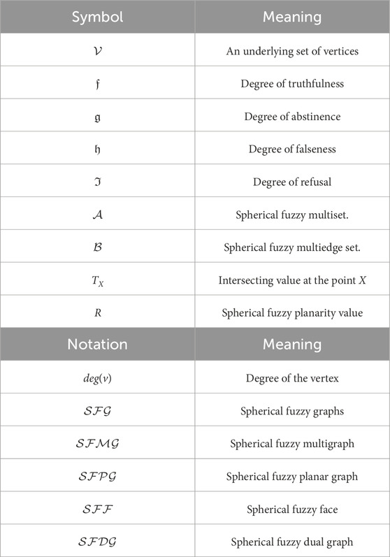
Some symbols and notations are used, which are presented in Table 2 along with their meanings.
3 Preliminaries
Definition 3.1. [1] Let
Example 3.2. Given the set
The fuzzy relation
The graph is shown in Figure 1.
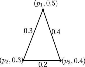
Figure 1. Fuzzy graph.
Definition 3.3. [28] Let
Definition 3.4. Let
Example 3.5. Let
The fuzzy multigraph is shown in Figure 2. There are two edges between
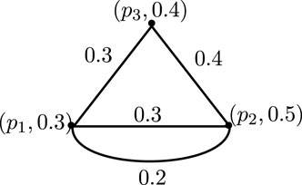
Figure 2. Fuzzy multigraph.
Definition 3.6. [26] Let the underlying set of vertices be
where
Moreover,
Example 3.7. Let
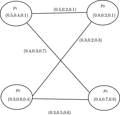
Figure 3. Spherical fuzzy graph
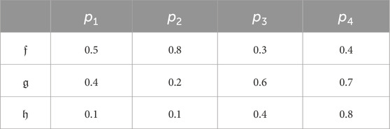
Table 1. Spherical fuzzy set

Table 2. Spherical fuzzy edge set
Definition 3.8. [26] Let the underlying set of vertices be
The orders of membership for truthfulness and abstinence are listed in descending order, but the sequence for falsehood may not follow the same order.
4 Spherical fuzzy planar graphs
Definition 4.1. [26] Let the underlying set of vertices be
for all
Example 4.2. In Figure 4, a
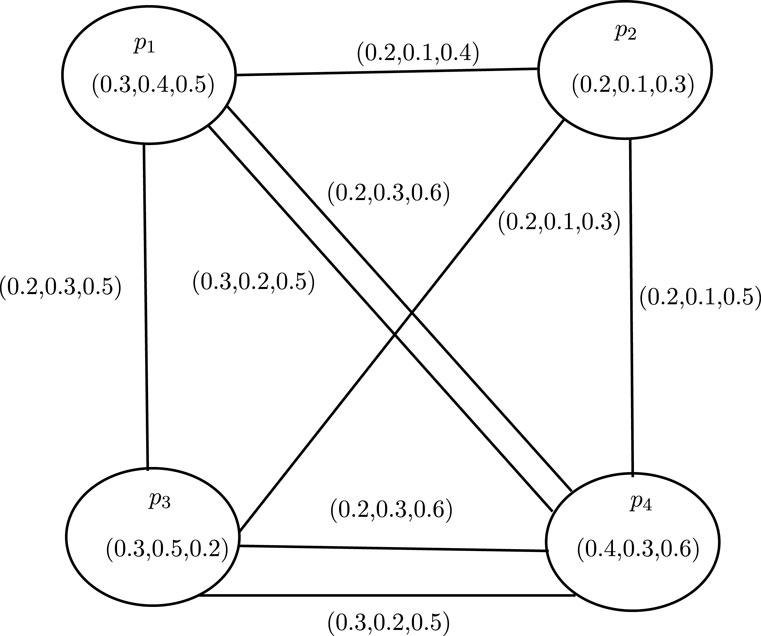
Figure 4.
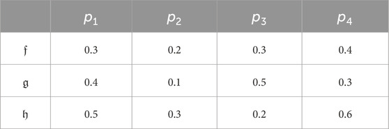
Table 3.

Table 4.
Definition 4.3. Let
for all
Example 4.4. In Example 4.2, the degrees of the vertices of
• deg
• deg
• deg
• deg
Definition 4.5. Let a spherical fuzzy multiedge set
in
and
for all
Example 4.6. Consider a
By direct computations, we can easily summarize that in this
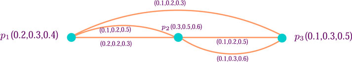
Figure 5.
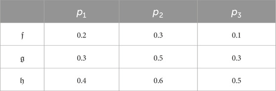
Table 5.

Table 6. Spherical fuzzy multiedge set
Definition 4 7. Let
be a spherical fuzzy multiedge set in
for all i = 1, 2, …, k and for all
Example 4.8. Let
Using basic calculations, from Figure 6, it is clear that it is complete
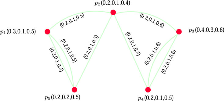
Figure 6. Complete

Table 7.
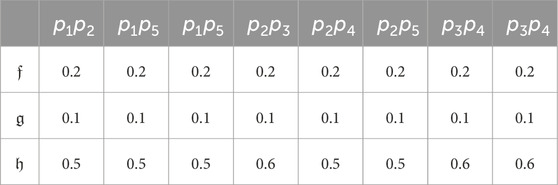
Table 8. Spherical fuzzy multiedge set
Definition 4.9. Strength of the spherical fuzzy edge
and can be calculated as given in Equation 2.
where i = 1, 2, …, k and for all
Example 4.10. Let
From Equation 2, the strength of the edges is computed as follows.
• For an edge
• For an edge
• For an edge
• For an edge
• For an edge
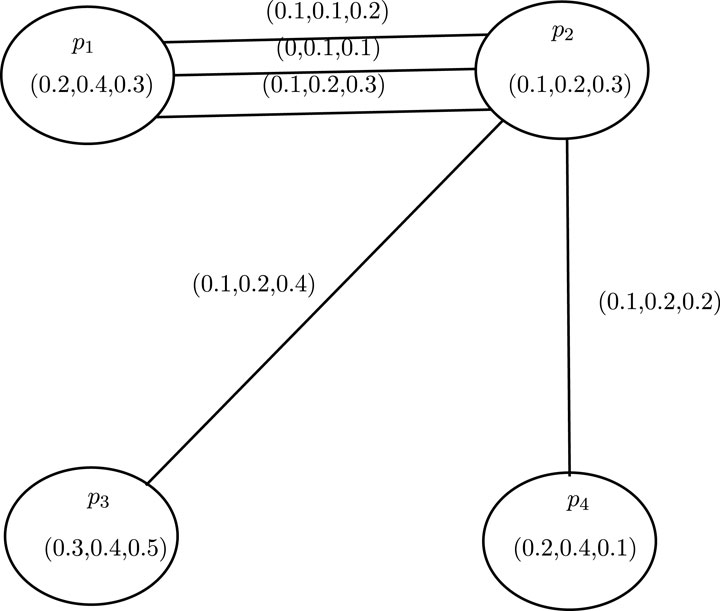
Figure 7.
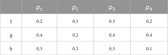
Table 9.

Table 10. Spherical fuzzy multiedge set
Definition 4.11. Let
Definition 4.12. Let
If the number of intersecting points increases, then the value of the planarity decreases. Thus, for
Example 4.13. Let
The intersecting value at the point
For an edge
By substituting the values from Tables 9, 10, we get Equation 5.
Similarly, for an edge
By putting the values from Tables 9, 10, we get Equation 6.
Substituting the values from Equations 8, 9 in Equation 7, we get the intersecting value as
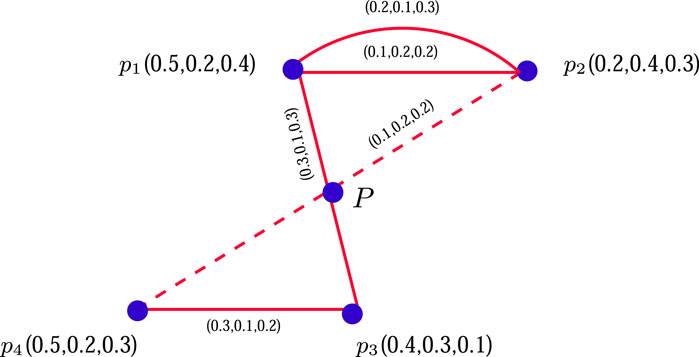
Figure 8.
Table 11.

Table 12. Spherical fuzzy multiedge set
Definition 4.14. For
Vividly,
Example 4.15. An
The intersecting value at the point
For an edge
By substituting the values from Tables 13, 14, we get
Similarly, for an edge
By putting the values from Tables 13, 14, we get
Substituting the values from Equations 8, 9 in Equation 7, we get intersecting value as
Figure 9.
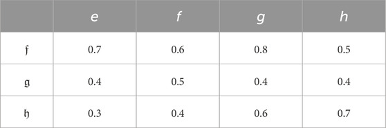
Table 13.

Table 14. Spherical fuzzy multiedge set
Theorem 4.16. Let
Proof. For complete
for all
and
In this way, for point
Here,
Definition 4.17. A
Theorem 4.18. For
Proof. Let
and
that is,
Example 4.19. Two
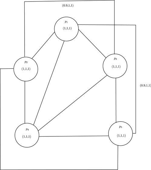
Figure 10. Example of strong
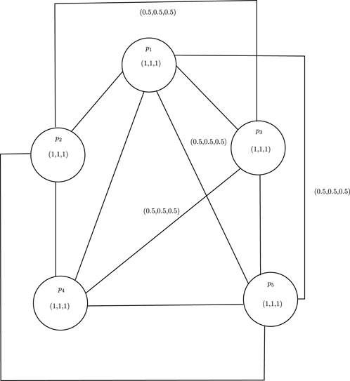
Figure 11. Example of not strong
Theorem 4.20. Let
Proof. A
The above theorem motivated to define the term strong planar graph.
Definition 4.21. A
Theorem 4.22. A
Proof. The
From Theorem 4.16, the value of planarity for complete
Definition 4.23. Let
and
Otherwise, it is not a considerable edge. For
Theorem 4.24. A
Proof. Let
Since
This implies that
and
This implies that
The crucial parameter of a
Definition 4.25. Let
for all
Definition 4.26. A
Example 4.27. Suppose
•
•
•
•Outer
Clearly, the values of truthfulness, abstinence, and falsehood of
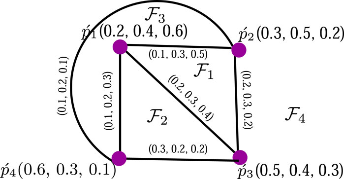
Figure 12. Faces of
5 Spherical fuzzy dual graph
The concept of duality is very useful in elaborating many models, like integrated circuits, drainage systems for basins, and others. A graph is planar if and only it has a dual graph. This means that for any planar graph, there exists a dual graph, and for any graph with dual graph, it must be planar. This concept works well to deal with a wide range of complicated and significant circumstances. By inspiring this concept, we are going to present the idea of a
Definition 5.1. Let
Let
and
respectively. Between two faces
Example 5.2. Let the underlying set of vertices
•
•
•
•
•
•
Here,
where the vertex
Thus, we get the values of truthfulness, abstinence, and falseness for the vertex
For vertex
For vertex
For vertex
For vertex
For vertex
Finally, for vertex
Now, the values of truthfulness, abstinence, and falseness of edges of
For an edge
For an edge
For an edge
For an edge
For an edge
For an edge
For an edge
For an edge
Thus, we get the edge set of
In Figure 13, the
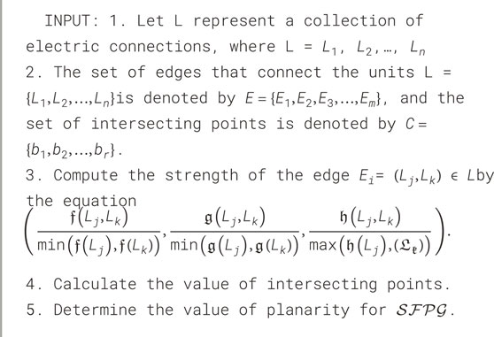
Algorithm 1. Method to calculate the value of planarity for electric connections.
Figure 13. Dual of
6 Application
In real-world power distribution systems, maintaining efficient and reliable connections between transformers and households is crucial. Using the spherical fuzzy multigraph model allows us to better visualize and optimize these complex networks. By representing transformers as vertices and the wires connecting them to households as edges, we can account for uncertainties or varying degrees of connectivity in the system. This approach provides insights into how power is distributed, identifies potential vulnerabilities, and suggests improvements in efficiency and reliability. In the example of a transformer system represented as a spherical fuzzy planar graph, the transformer is considered a node and the electrical connections (wires) between components are treated as edges. The number of intersecting points (where wires cross) directly impacts the damage rate. The more intersections there are, the higher the likelihood of damage, as each crossing increases the risk of overheating or failure. Using the spherical fuzzy graph, we can model the uncertainty and degree of risk associated with each connection, helping minimize the damage rate by optimizing the placement of wires and reducing intersections. A vertex denotes each transformer
Figure 14. Transformer unit connections.
The rate of decomposition grows with the number of crossings.
Thus, the spherical fuzzy planarity value
Figure 15. Spherical fuzzy electric connection model.
6.1 Comparison with already existing methods
There are already existing methods, such as fuzzy planar graph and interval-valued planar graph, which can be used to determine if a discrete process is planar or if an interval representing a continuous process is planar, respectively. However, spherical planar graphs can be understood by combining principles from spherical fuzzy sets and planar graphs.
In planar graphs, interval-valued planar graphs are considered simultaneously [40]. However, we use a more versatile technique that involves three types of degree of membership such as truthfulness, falseness, and abstinence memberships, which gives more clear information about uncertain data.
7 Limitation and advantages
The proposed technique of spherical planar graph is restricted to undirected graphs only.
The spherical fuzzy planar graph extends traditional fuzzy graph theory by incorporating membership, non-membership, and hesitancy degrees, offering a more comprehensive representation of uncertainty. Compared to standard fuzzy graphs, it provides higher precision in modeling ambiguous or imprecise relationships. Its planar structure simplifies visualization and analysis of complex networks, reducing computational complexity. The approach supports dynamic adaptability, making it suitable for systems with evolving uncertainties. It also enhances decision-making capabilities by capturing partial truths more effectively than traditional fuzzy models. Furthermore, its multi-dimensional representation is particularly useful for handling conflicting and incomplete information in engineering and optimization problems. The proposed study, applying spherical fuzzy planar graphs to transformer systems, effectively models uncertain and dynamic connections between components like wires and nodes. It can address network reliability analysis, fault detection, and load balancing in power systems by capturing imprecise data and ambiguous relationships. This approach also aids in optimizing energy distribution and minimizing losses through flexible modeling of uncertainty. Additionally, it supports scalability and adaptability, making it suitable for evolving smart grid systems and renewable energy integration challenges.
8 Conclusion
Graph theory has enormous applications to problems in transportation, operations research, computer science, image capture, data mining, etc. Sometimes, to deal with uncertainty and vagueness in various network problems, various graph theoretical concepts are used based on Zadeh’s fuzzy relations.
Soft fuzzy planar graphs, vague planar graphs, hesitant
Data availability statement
The raw data supporting the conclusions of this article will be made available by the authors, without undue reservation.
Author contributions
HG: conceptualization and writing–original draft. SH: project administration, supervision, and writing–original draft. Sadaf: investigation, methodology, and writing–original draft. AK: project administration and writing–review and editing. JS: data curation, supervision, and writing–review and editing.
Funding
The author(s) declare that financial support was received for the research, authorship, and/or publication of this article. This work was supported by the National Natural Science Foundation of China (No. 62407011).
Conflict of interest
The authors declare that the research was conducted in the absence of any commercial or financial relationships that could be construed as a potential conflict of interest.
Publisher’s note
All claims expressed in this article are solely those of the authors and do not necessarily represent those of their affiliated organizations, or those of the publisher, the editors and the reviewers. Any product that may be evaluated in this article, or claim that may be made by its manufacturer, is not guaranteed or endorsed by the publisher.
References
2. Yager RR. Pythagorean membership grades in multi-criteria decision making. IEEE Trans Fuzzy Syst (2014) 22(4):958–65. doi:10.1109/tfuzz.2013.2278989
3. Samanta S, Akram M, Pal M. m-Step fuzzy competition graphs. J Appl Mathematics Comput (2014) 47:461–72. doi:10.1007/s12190-014-0785-2
4. Cuong BC. Picture fuzzy sets-First results, Part 2. In: Seminar neuro-fuzzy systems with applications. Hanoi, Vietnam: Institute of Mathematics, Vietnam Academy of Science and Technology (2013).
5. Gundogdu FK, Kahraman C. It Spherical fuzzy sets and spherical fuzzy TOPSIS method. J Intell Fuzzy Syst (2018) 36:1–36. doi:10.3233/JIFS-181401
6. Ashraf S, Abdullah S, Mahmood T, Mahmood F. Spherical fuzzy sets and their applications in multi-attribute decision making problems. J Intell Fuzzy Syst (2018) 36:2829–44. doi:10.3233/JIFS-172009
7. Ashraf S, Abdullah S, Mahmood T. Spherical fuzzy Dombi aggregation operators and their application in group decision making problems. J Ambient Intell Humaniz Comput (2019) 11:2731–49. doi:10.1007/s12652-019-01333-y
8. Zadeh LA. Similarity relations and fuzzy orderings. Inf Sci (1971) 3(2):177–200. doi:10.1016/s0020-0255(71)80005-1
10. Rosenfeld A. Fuzzy graphs. In: Fuzzy sets and their applications. New York, NY, USA: Academic Press (1975). p. 77–95.
11. Bhattacharya P. Some remarks on fuzzy graphs. Some remarks fuzzy graphs, Pattern Recognition Lett (1987) 6(5):297–302. doi:10.1016/0167-8655(87)90012-2
12. Mordeson JN, Peng CS. Operations on fuzzy graphs. Inf Sci (1994) 79:159–70. doi:10.1016/0020-0255(94)90116-3
13. Nagoorgani A, Malarvizhi J. Isomorphism on fuzzy graphs. World Acad Sci Eng Techn (2008) 23:505–11.
15. Shannon A, Atanassov KT. A first step to a theory of the intuitionistic fuzzy graphs (1994). In: D Lakov, Editor Proceeding of the FUBEST. Sofia, Bulgaria: Springer 59–61.
16. Parvathi R, Karunambigai MG, Atanassov KT. Operations on intuitionistic fuzzy graphs. In: Proceedings of the IEEE international conference on fuzzy systems (2009). p. 1396–401.
17. Akram M, Alshehri NO. Intuitionistic fuzzy cycles and intuitionistic fuzzy trees. The Scientific World J (2014) 2014:305836. doi:10.1155/2014/305836
18. Akram M, Alshehri NO, Dudek WA. Certain types of interval-valued fuzzy graphs. J Appl Mathematics (2013) 2013:1–11. Article ID 857070. doi:10.1155/2013/857070
19. Akram M, Dudek WA. Intuitionistic fuzzy hypergraphs with applications. Inf Sci (2013) 218:182–93. doi:10.1016/j.ins.2012.06.024
20. Akram M, Davvaz B. Strong intuitionistic fuzzy graphs. Filomat (2012) 26(1):177–96. doi:10.2298/fil1201177a
21. Alshehri N, Akram M. Intuitionistic fuzzy planar graphs. Discret Dyn Nat Soc (2014) 9:397823. doi:10.1155/2014/397823
22. Naz S, Ashraf S, Akram M. A novel approach to decision-making with Pythagorean fuzzy information. Mathematics (2018) 6(95):95. doi:10.3390/math6060095
23. Akram M, Naz S. Energy of Pythagorean fuzzy graphs with applications. Mathematics (2018) 6(136):136. doi:10.3390/math6080136
24. Akram M, Habib A, Ilyas F, Dar JM. Specific types of pythagorean fuzzy graphs and application to decision-making. Math Comput Appl (2018) 23(42):42. doi:10.3390/mca23030042
25. Akram M, Dar JM, Naz S. Certain graphs under pythagorean fuzzy environment. Complex Intell. Syst. (2019) 5:127-144.
26. Akram M, Saleem D, Al-Hawary T. Spherical fuzzy graphs with application to decision-making. Math Comput Appl (2020) 300(25):8. doi:10.3390/mca25010008
27. Yahya MS, Mohamed AA. Energy of spherical fuzzy graphs. Adv Math Scientific J (2020) 321–32. doi:10.37418/amsj.9.1.26
28. Yager RR. On the theory of bags. Int J Gen Sys (1986) 13(1):23–37. doi:10.1080/03081078608934952
29. Pal A, Samanta S, Pal M. Concept of fuzzy planar graphs. In: proceedings of the Science and Information Conference; London (2013). p. 557–63.
30. Samanta S, Pal M, Pal A. New concepts of fuzzy planar graphs. Int J Adv Res Artif Intelligence (2014) 3(1):52–9. doi:10.14569/ijarai.2014.030108
31. Pramanik T, Samanta S, Pal M. Special planar fuzzy graph configurations. Int J Sci Res Publ (2012) 2:1–4.
32. Akram M, Samanata S, Pal M. Application of bipolar fuzzy sets in planar graph. Int J Appl Comput Math (2017) 3:773–85. doi:10.1007/s40819-016-0132-4
33. Nirmala G, Dhanabal K. Interval-valued fuzzy planar graphs. Int J Mach Learn Cybern (2016) 7:654–64. doi:10.1007/s13042-014-0284-7
34. Ahmad U, Nawaz I. Directed rough fuzzy graph with application to trade networking. Comput Appl Mathematics (2022) 41(8):366. doi:10.1007/s40314-022-02073-0
35. Ahmad U, Batool T. Domination in rough fuzzy digraphs with application. Soft Comput (2023) 27(5):2425–42. doi:10.1007/s00500-022-07795-1
36. Ahmad U, Khan NK, Saeid AB. Fuzzy topological indices with application to cybercrime problem. Granular Comput (2023) 8:967–80. doi:10.1007/s41066-023-00365-2
37. Ahmad U, Nawaz I. Wiener index of a directed rough fuzzy graph and application to human trafficking. J Intell and Fuzzy Syst (2023) 44:1479–95. doi:10.3233/jifs-221627
38. Ahmad U, Sabir M. Multicriteria decision-making based on the degree and distance-based indices of fuzzy graphs. Granular Comput (2022) 8:793–807. doi:10.1007/s41066-022-00354-x
39. Muhiuddin G, Hameed S, Maryam A, Ahmad U. Cubic pythagorean fuzzy graphs. J Mathematics (2022) 2022:1144666. doi:10.1155/2022/1144666
40. Muhiuddin G, Hameed S, Rasheed A, Ahmad U. Cubic planar graph and its application to road network. Math Probl Eng (2022) 2022:1–12. doi:10.1155/2022/5251627
41. Kosari S, Rao Y, Jiang H, Liu X, Wu P, Shao Z. Vague graph structure with application in medical diagnosis. symmetry (2020) 12(10):1582. doi:10.3390/sym12101582
42. Shi X, Kosari S. Certain properties of domination in product vague graphs with an application in medicine. Front Phys (2021) 9:680634. doi:10.3389/fphy.2021.680634
43. Qiang X, Akhoundi M, Kou Z, Liu X, Kosari S. Novel concepts of domination in vague graphs with application in medicine. Math Probl Eng (2021) 2021:1–10. doi:10.1155/2021/6121454
44. Shi X, Kosari S, Talbi AA, Sadati SH, Rashmanlou H. Investigation of the main energiesof picture fuzzy graph and its applications. Int J Comput Intelligence Syst (2022) 15(1):31. doi:10.1007/s44196-022-00086-5
45. Rao Y, Binyamin MA, Adnan A, Mehtab M, Fazal S. On the planarity og graphs associated with symmetric and pseudo symmetric numerical semigroups. Mathematics (2023) 11(7):1681. doi:10.3390/math11071681
46. Shao Z, Kosari S, Rashmanlou H, Shoaib M. New concepts in intuitionistic fuzzy graph with application in water supplier systems. Mathematics (2020) 8:1241. doi:10.3390/math8081241
47. Shao Z, Kosari S, Rashmanlou H, Shoaib M. Certain concepts of vague graphs with applications to medical diagnosis. Frontier Phys (2020) 8:357. doi:10.3389/fphy.2020.00357
48. Shi X, Kosari S, Ahmad U, Hameed S, Akhter S. Evalution of various topological indices of flabellum graphs. Mthematics (2023) 11(19):1167. doi:10.3390/math11194167-5October2023
Keywords: spherical fuzzy multigraph, spherical fuzzy planar graph, spherical fuzzy planarity value, spherical fuzzy dual graph, fuzzy graph theory
Citation: Guan H, Hameed S, Sadaf , Khan A and Shafi J (2025) A spherical fuzzy planar graph approach to optimize wire configuration in transformers. Front. Phys. 13:1413813. doi: 10.3389/fphy.2025.1413813
Received: 07 April 2024; Accepted: 27 January 2025;
Published: 19 March 2025.
Edited by:
Igor Kondrashuk, University of Bío-Bío, ChileReviewed by:
Sarfraz Ahmad, COMSATS University Islamabad, Lahore Campus, PakistanUgur Kadak, Gazi University, Türkiye
Copyright © 2025 Guan, Hameed, Sadaf, Khan and Shafi. This is an open-access article distributed under the terms of the Creative Commons Attribution License (CC BY). The use, distribution or reproduction in other forums is permitted, provided the original author(s) and the copyright owner(s) are credited and that the original publication in this journal is cited, in accordance with accepted academic practice. No use, distribution or reproduction is permitted which does not comply with these terms.
*Correspondence: Saira Hameed, c2FpcmEubWF0aEBwdS5lZHUucGs=