A homophilic and dynamic influence maximization strategy based on independent cascade model in social networks

Influence maximization (IM) is crucial for recommendation systems and social networks. Previous research primarily focused on static networks, neglecting the homophily and dynamics inherent in real-world networks. This has led to inaccurate simulations of information spread and influence propagation between nodes, with traditional IM algorithms’ selected seed node sets failing to adapt to network evolution. To address this issue, this paper proposes a homophilic and dynamic influence maximization strategy based on independent cascade model (HDIM). Specifically, HDIM consists of two components: the seed node selection strategy that accounts for both homophily and dynamics (SSHD), and the independent cascade model based on influence homophily and dynamics (ICIHD). SSHD strictly constrains the proportions of different node types in the seed node set and can flexibly update the seed node set when the network structure changes. ICIHD redefines the propagation probabilities between nodes, adjusting them in response to changes in the network structure. Experimental results demonstrate HDIM’s excellent performance. Specifically, the influence range of HDIM exceeds that of state-of-the-art methods. Furthermore, the proportions of various activated nodes are closer to those in the original network.

1 Introduction

With the continuous evolution of the Internet, social media has become a primary medium for individuals to express opinions and communicate with others, leading to a plethora of research on social networks [1–3]. User interactions, sharing, and comments on social network platforms directly affect other users. When seeking new job opportunities, individuals tend to look for relevant information on specialized recruitment websites. Meanwhile, many companies leverage social media to disseminate their recruitment advertisements and brand information. As a result, influence maximization (IM) has become a significant research area in social networks [4], garnering widespread attention, particularly in fields such as public opinion analysis, recommendation systems, and epidemic propagation. The core objective of IM is to identify and target a group of users within a social network who can most effectively propagate information. For example, in the context of corporate recruitment, companies disseminating job advertisements through social networks need to precisely target the most promising user groups to ensure effective dissemination of information. To identify these most promising users, IM research is required.

Current IM algorithms [5, 6] have made significant progress in Enhancing information dissemination. These algorithms utilize the connection relationships between nodes in the network and the evaluation of node influence to determine the most promising spreading nodes. However, these algorithms primarily focus on the structure of a single network and node influence, overlooking homophily in real networks [7]. Homophily in social networks encompasses both structural homophily and influence homophily. Structural homophily refers to the similarity in connection patterns or topological structures among nodes in a social network. In other words, structural homophily describes the degree of pattern similarity in the relationship network among nodes. In a social network with structural homophily, the connections between nodes may exhibit some degree of clustering phenomenon, where nodes tend to connect with other nodes with similar attributes or interests. Influence homophily refers to the similarity in influence propagation between nodes in a social network. This homophily indicates that in social networks, certain nodes may be more easily influenced by similar nodes, leading to similar patterns of information or behavior propagation in the network. Therefore, ignoring homophily may result in the ineffectiveness or poor performance of IM algorithms.

Moreover, current research [8] often focuses on static social networks, where the nodes and their connections remain unchanged. However, real-life social networks are dynamic and change over time. With time, old nodes and connections may disappear, while new nodes and connections may join, exhibiting certain regularities [9]. For example, Barabási et al. [10] proposed a scale-free network generation model, describing the regularities in node connections in social networks. Therefore, traditional seed node selection strategies based on static social networks may not be applicable to dynamic social networks. In dynamic social networks, the importance and influence of nodes change over time. To address this issue, a series of corresponding seed node sets need to be selected based on the continuous changes in the social network.

To address the issue that traditional IM algorithms overlook homophily and dynamics, we propose a homophilic and dynamic influence maximization strategy based on independent cascade model (HDIM). Specifically, concerning the homophily of social networks, HDIM first classifies users based on user attributes since users with similar attributes are more likely to connect and influence each other. By selecting different types of users as seed nodes, it can ensure that the influence covers different types of user groups. Furthermore, HDIM further considers the propagation process of influence between users in real social networks. The probability of mutual influence between users not only depends on their connection relationships but also on their attribute similarity. Regarding the dynamics of social networks, we propose a method that combines network changes to update seed users. In other words, HDIM focuses on users in the network that undergo changes to ensure that its selections can adapt to network evolution. Compared to reapplying seed node selection strategies, this approach significantly saves computational time and can more effectively address changes in network structure. Additionally, since changes in network structure affect the propagation probabilities between users, HDIM can dynamically adjust the influence propagation model to better adapt to network changes. The specific contributions of this paper are as follows.

$•$ We propose a seed node selection strategy considering homophily and dynamics (SSHD). Firstly, SSHD imposes strict constraints on seed nodes. The proportions of different types of seed nodes in the seed node set are determined by their proportions among nodes in the initial network. Secondly, we introduce a degree discount heuristic strategy in a directed graph (DDD) to compute node degree discount scores. When the network structure changes, SSHD combines previously selected seed nodes with the changing nodes to flexibly update the seed node set.

$•$ We propose an independent cascade model based on influence homophily and dynamics (ICIHD). ICIHD redefines the propagation probabilities between nodes, making these probabilities dependent not only on the network topology but also on influence homophily parameters. Influence homophily parameters refer to the likelihood that nodes with similar attributes influence each other. Additionally, as the network structure changes, the propagation probabilities between nodes also change accordingly.

$•$ Extensive experimental results demonstrate the outstanding performance of HDIM. Specifically, in four different static social networks, although HDIM activates slightly fewer nodes than greedy algorithms, the proportions of various activated nodes are closer to those in the initial network. In dynamic social networks, HDIM exhibits better adaptability than other baseline methods. With changes in social networks, HDIM’s influence range is approximately 60 nodes larger than state-of-the-art methods. Moreover, concerning methods considering network dynamics, HDIM performs equally well in terms of influence range but achieves superior proportions of various activated nodes. The source code is available at: https://github.com/Wijipedia/HDIM.

The remaining organization of this paper is as follows: Section 2 summarizes previous work. Section 3 introduces some preparatory knowledge related to HDIM. Section 4 provides a detailed description of HDIM. Section 5 presents experimental results and detailed analysis. Finally, Section 6 concludes the work of this paper and proposes future prospects.

2 Related work

2.1 Influence maximization

Domingos et al. [11] conceptualized the market as a social network and recognized the importance of understanding how customers influence each other within this network. They were the first to discover and study the additional value of customers. Kempe et al. [12] further elucidated the well-known problem of IM. They also proposed two notable algorithms known as the greedy algorithm and the heuristic algorithm. Leskovec et al. [13] introduced the cost-effective lazy forward (CELF) optimization method based on the submodular properties of IM objectives. They addressed the inefficiency issue of the greedy algorithm. Heidari et al. [14] proposed a state machine greedy algorithm, addressing the scalability problem of traditional greedy algorithms. It enabled the application of greedy algorithms in large-scale social networks. Chen et al. [15] proposed a risk-free variant of the adaptive greedy algorithm, which never performs worse than non-adaptive greedy algorithms.

Heuristic algorithms aim to find a suitable set of seed nodes in a graph based on some strategy. Compared to greedy algorithms, heuristic algorithms significantly improve time efficiency. However, the performance of heuristic algorithms cannot be guaranteed. Chen et al. [16] introduced a Degree Discount Heuristic algorithm, which has higher accuracy compared to degree-based heuristic algorithms. Zhang et al. [17] proposed a PageRank-inspired heuristic approach. This heuristic solution explicitly reduces the influence of individuals connected to the selected seed nodes. By integrating this discount mechanism, the algorithm achieves performance comparable to greedy algorithms. Jia et al. [18] proposed a three-phase heuristic algorithm for social network IM. The algorithm considers the impact of influence overlap on its effectiveness, striking a balance between algorithm effectiveness and time efficiency.

Furthermore,

2.2 Homophily

Kossinets et al. [19] pointed out a difference between social networks and other networks, which is homophily. Aral et al. [20] demonstrated that ignoring homophily could lead to a significant overestimation of the effectiveness of seeding strategies. Xie et al. [21] proposed a competitive IM method considering inactive nodes and community homophily. They broke down barriers to information propagation between different communities. Chen et al. [22] proposed a community-based IM algorithm based on the structural attributes of the community. They formulated corresponding strategies for homophily when selecting seed nodes. However, they only considered the influence range in the final result. M.S. et al. [23] proposed a greedy algorithm that simultaneously considers maximizing the number of nodes and influence balance while retaining the attractive theoretical guarantees of traditional IM algorithms.

2.3 Dynamic social networks

Sheng et al. [24] tackled the dynamic IM problem by transforming each node in the network into low-dimensional vector representations using network representation learning. They then addressed the dynamic IM problem in the low-dimensional latent space. Song et al. [25] proposed an upper-bound alternating greedy algorithm. They solved the seed selection problem in dynamic social networks by tracking a set of influential nodes and replacing them based on network changes. Zhang et al. [26] introduced a novel framework for IM based on prediction and replacement. This framework first predicts future network snapshots using historical network snapshot information. Then, based on the prediction results, it mines seed nodes suitable for dynamic networks. Li et al. [27] proposed an adaptive agent-based evolutionary method. They utilized an adaptive solution optimizer to drive the evolutionary process and optimize the selection of seed sets in dynamic environments. Chandran et al. [28] proposed the dynamic traceable set method to track individual node influence changes over time as the network topology evolves.

2.4 Influence diffusion models

Influence diffusion models [12] primarily consist of two main types: linear threshold models and independent cascade models. Jendoubi et al. [29] proposed two evidence-based model for IM on Twitter. This model uses belief function theory to estimate user influence. Wang et al. [30] introduced a novel influence network embedding method and a new IM algorithm based on network representation learning. The probability of information propagation between network nodes differs from other network representation learning methods based on random walks. Li et al. [31] proposed a multi-factor information diffusion model by considering multiple factors in information propagation. Bozorgi et al. [32] provided nodes with decision-making capabilities regarding incoming influence propagation. Considering the existence of numerous competitors in real life, they proposed a competitive linear threshold model. Li et al. [33] modeled social networks in multi-dimensional space and proposed a propagation simulation based on the Gaussian propagation model. Additionally, Guo et al. [34] proposed an influence maximization algorithm based on group trust and local topology structure. This algorithm optimizes the propagation process by defining concepts such as group connectivity, inter-group diffusion, and group trust, while incorporating local structural information. Yang et al. [35] considered the potential impact of entity correlations in real-world social networks on information diffusion, proposing a balanced influence maximization framework based on deep reinforcement learning.While these methods account for various factors in simulating information propagation in real social networks, they overlook two important properties: homophily and dynamics.

3 Preliminaries

In this section, we introduce key definitions and symbols.

3.1 Influence maximization in static social networks

IM in static social networks involves selecting a certain number of initial nodes, known as seed nodes, from a given set of nodes. These seed nodes aim to activate as many nodes as possible through an influence diffusion model.

Kempe et al. [12] formalized this problem as follows: Given a network $G=(V,E)$, where $V$ represents the set of nodes in the graph and $E$ represents the set of edges. Given an influence propagation model and a positive integer $k$, the IM problem is to find $k$ nodes such that the number of nodes influenced by these nodes is maximized under the current propagation model. The objective function of IM is shown in Equation 1.

$S^{*}=argmax\left(\sigma \left(S\right)\right)S\subseteq V,|S|=k(1)$

Here, $S$ represents the set of seed nodes containing $k$ nodes. The number of users influenced by the nodes in set $S$ represents the influence capacity of $S$. $\sigma (S)$ denotes the number of users influenced by the nodes in set $S$. $S^{*}$ represents the set $S$ with the strongest influence capacity.

3.2 Influence maximization in dynamic social networks

Dynamic social networks refer to a series of static network graphs where nodes and edges change over time. Each static network graph represents the state of the social network at a specific time point. To facilitate research, we discretize time and set a small time interval during which the network topology changes. Therefore, based on the traditional IM problem in static social networks described above, we can define IM in dynamic social networks as follows:

$\mathbf{D}\mathbf{e}\mathbf{fi}\mathbf{n}\mathbf{i}\mathbf{t}\mathbf{i}\mathbf{o}\mathbf{n}\mathbf{1}$: Influence Maximization in Dynamic Social Networks: Given $G_t(V_t,E_t)$ as the social network at time $t$, where the nodes and edges of the network $G_t$ at time $t$ are fixed, but they evolve over time. Forming a dynamic social network when $t=\mathrm{0,1},\dots ,n$, the objective in IM in dynamic social networks is to find the optimal set of seed nodes in the graph corresponding to each time $t$. We formalize the IM problem in dynamic social networks as shown in Equation 2.

$S_t^{*}=argmax\left({\sigma }_t\left(S_t\right)\right)S_t\subseteq V_t,|S_t|=k,t=\mathrm{0,1},\dots ,n.(2)$

Here, $S_t$ represents the set of seed nodes containing $k$ nodes at time $t$. ${\sigma }_t(S_t)$ represents the number of nodes influenced by the nodes in set $S_t$ at time $t$. $S_t^{*}$ represents the set $S_t$ with the strongest influence capacity at time $t$.

4 Methodology

4.1 Framework

In this section, we first provide a brief overview of the overall framework of HDIM, as illustrated in Figure 1. Then, we delve into each component of HDIM in detail.

Figure 1

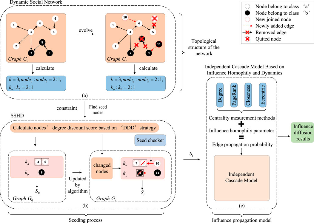
Figure 1. The overall framework of HDIM. (A) The topological structure of the directed graph representing the social network. (B) The process of selecting the corresponding seed nodes in the dynamic social network. (C) The independent cascade model based on influence homophily and dynamics.

Figure 1A illustrates the topological structure of the directed graph representing the social network. Firstly, we classify the nodes based on their attributes. In this study, we categorize them into two categories based on the users’ gender. Category ’a’ includes white nodes, which constitute a larger proportion, while category ’b’ comprises black nodes, occupying a smaller proportion. Then, we depict the dynamic nature of the social network. That is, at a certain timestamp, the nodes and edges remain fixed. However, over time, new nodes and edges may join the network, while old nodes and associated edges may disappear.

Figure 1B describes how to select the corresponding seed nodes in a dynamic social network. We establish the DDD to search for seed nodes. In addition to providing the number of seed nodes $k$, we also consider the homophily of the social network and provide constraints. The seed nodes at timestamp $t$ are jointly updated by the seed node set from the previous timestamp and the changed nodes. The role of the seed checker is to compare the degree discount scores of the changed nodes with the seed nodes from the previous timestamp. Then, it decides whether to replace the existing seed nodes.

Figure 1C illustrates the influence propagation model. Unlike the traditional independent cascade model, ICIHD model considers the homophily and dynamics of the social network. Considering the realistic scenario of influence propagation between nodes, the influence propagation probability between nodes depends not only on the network topology but also on the node’s attributes. Due to the changes in the seed node set, this model can dynamically output the nodes influenced by the seed node set.

4.2 Degree discount heuristic strategy in directed graphs

The degree discount heuristic in an undirected graph [16] is an improvement upon the basic degree heuristic strategy. Suppose node $j$ is a neighbor of node $i$, and node $j$ has already been selected as a seed node. When considering whether to choose node $i$ as a seed node based on a degree-based selection strategy, the edge $(i,j)$ should be discounted because node $i$ cannot generate additional influence on node $j$. If there is an edge between two nodes, it indicates that influence can propagate bidirectionally through that edge. Once a node is confirmed as a seed node, the degree discount score of its neighboring nodes will be updated using Equation 3.

$d{d}_v=d_v-2t_v-\left(d_v-t_v\right)t_{v}p(3)$

Where $d{d}_v$ represents the degree discount score of node $v$, $d_v$ denotes the degree of node $v$, and $t_v$ indicates the number of seed nodes among the neighboring nodes of node $v$. $p$ is the probability parameter for edges, representing the probability of influence propagating to neighboring nodes through edges.

However, in a directed graph, influence can only propagate from one node to the nodes it points to. The out-degree of a node refers to the number of edges emanating from that node. Each outgoing edge signifies the potential influence or information transmission from the node to its neighboring nodes. Thus, a higher out-degree indicates that the node has the potential to influence more nodes in the graph. In this scenario, there may exist three types of connections between nodes, as shown in Figure 2.

1. As shown in Figure 2A, node $j$ is a seed node pointing to node $i$. Since node $i$ cannot activate node $j$ (there is no edge from $i$ to $j$ in the graph), the degree discount score of node $i$ does not need to consider node $j$.

2. As shown in Figure 2B, node $j$ is a seed node, and $i$ points to $j$. Although in this case node $i$ may activate node $j$ (there is an edge from $i$ to $j$ in the graph), node $j$ has already been previously selected as a seed node. In the independent cascade model, nodes only attempt to activate their inactive neighboring nodes. Therefore, when computing the degree discount score of node $i$ in this scenario, we should not consider the edge $(i,j)$.

3. As shown in Figure 2C, node $j$ is a seed node, and the connection between $i$ and $j$ is bidirectional. The probability that node $j$ activates node $i$ is $p(j,i)$. In this case, selecting node $i$ as a seed node does not add any extra influence (the contribution to the expected influence is 0). The probability that node $i$ is not activated by node $j$ is $1-p(j,i)$. When node $i$ is chosen as a seed node, the number of nodes it can activate is $1+p(i,v)$. Therefore, the expected influence when node $i$ is selected as a seed node is $(1-p(j,i))(1+p(i,v))$. When $j$ is not a seed node, the expected influence generated by $i$ being a seed node is $1+p(i,j)+p(i,v)$. Let $A=(1-p(j,i))(1+p(i,v))$ and $B=1+p(i,j)+p(i,v)$. Assuming $\gamma$ is the degree discount of $i$ to seed node $j$ (i.e., the discount of edge $(i,j)$), then $p(i,j)\gamma =B-A$, $\gamma =\frac{B-A}{p(i,j)}$. We can compute the degree discount score of node $i$ using Equation 4.

$d{d}_i=d_{\mathit{out}}\left(i\right)-\gamma (4)$

Where $d_{\mathit{out}}(i)$ represents out-degree of node $i$.

Figure 2

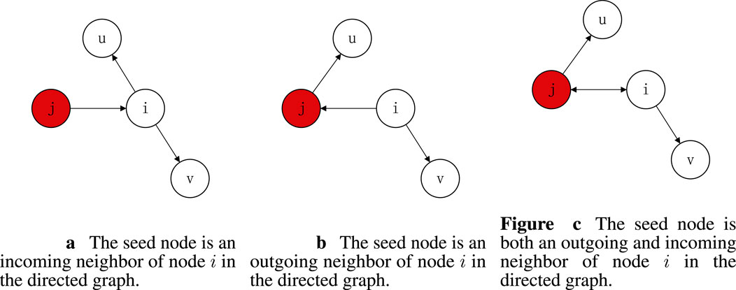
Figure 2. (A) The seed node is an incoming neighbor of node $i$ in the directed graph. (B) The seed node is an outgoing neighbor of node $i$ in the directed graph. (C) The seed node is both an outgoing and incoming neighbor of node $i$ in the directed graph. There are three cases in the directed graph, among which the seed node is a neighbor node of a certain node.

In directed graphs, degree discounting only occurs between nodes with bidirectional edges. Therefore, in Figure 2C, when there are $s$ nodes like $j$ in the neighborhood of node $i$, we can compute the degree discount score of $i$ using Equations 5–8. For convenience of representation, we assume that the edge propagation probability between nodes is $p$.

$A^{\prime }={\left(1-p\right)}^s\left(1+\left(d_{\mathit{out}}\left(i\right)-s-s_{\mathit{out}}\left(i\right)\right)p\right)(5)$

$B^{\prime }=1+\left(d_{\mathit{out}}\left(i\right)-s_{\mathit{out}}\left(i\right)\right)p(6)$

${\gamma }^{\prime }=\frac{B^{\prime }-A^{\prime }}{sp}(7)$

$d{d}_i^{\prime }=d_{\mathit{out}}\left(i\right)-s{\gamma }^{\prime }-s_{\mathit{out}}\left(i\right)(8)$

Where $s_{\mathit{out}}(i)$ represents the number of neighboring nodes that node $i$ points to, which are already seed nodes. Based on the above explanation, when calculating the number of active nodes, we should subtract those nodes that have already become seed nodes from the out-degree neighboring nodes.

Algorithm 1

Algorithm 1. Calculation of node degree discount score in directed graph.

In the DDD, we prioritize selecting nodes with higher degree discount scores as seed nodes. The calculation of the degree discount score for nodes is illustrated in Algorithm 1. Here, $s_{\mathit{out}}(u)$ represents the number of seed nodes among the out-degree neighboring nodes of node $u$, $s$ represents the number of nodes in the out-degree and in-degree neighboring nodes of node $u$ that are both seed nodes. $Ne{i}_{\mathit{out}}(u)$ denotes the out-degree neighboring nodes of node $u$, and $Ne{i}_{in}(u)$ represents the in-degree neighboring nodes of node $u$. The expected influence computed in steps 10 and 11 is different. The expected influence calculated in step 10 represents the expected influence when selecting node $u$ with seed nodes present among bidirectional neighboring nodes. The expected influence calculated in step 11 represents the expected influence when selecting node $u$ without seed nodes present among bidirectional neighboring nodes.

4.3 Seed node selection strategy considering homophily and dynamics

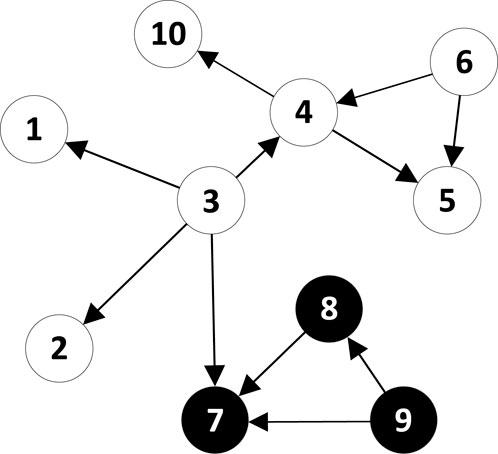
We propose a seed node selection strategy that takes into account the homophily and dynamics of social networks. When considering homophily, we impose constraints on selecting seed nodes. The proportion of the two types of nodes in the seed node set should be consistent with their proportion in the initial network. This is because similar nodes are more likely to connect and influence each other. By controlling the seed set, we aim to achieve influence across both types of nodes. For example, in Figure 3, we categorize nodes into two types: white nodes and black nodes. Let’s assume we need to select three seed nodes. Initially, with no seed nodes selected, we choose nodes based on their out-degree. Node 3 has an out-degree of 4. So, we first select node 4 as a seed node. Nodes 4, 6, and 9 have out-degrees of 2. We also need to randomly select two of them as seed nodes. Without constraints on seed node selection, node 9 might not be chosen. This could result in almost no active black nodes. This not only harms the interests of black nodes but may also lead to a reduction in the influence range. However, with constraints on seed node selection, we can avoid this issue. Since the ratio of white nodes to black nodes is $2:3$, the proportion in the seed node set remains consistent. We choose two white nodes and one black node as seed nodes. Node 9 becomes a forced selection. Thus, we achieve the goal of influence reaching both types of nodes simultaneously while still ensuring the influence range.

Figure 3

Figure 3. The directed social network after node categorization.

Algorithm 2

Algorithm 2. Constraint for seed nodes.

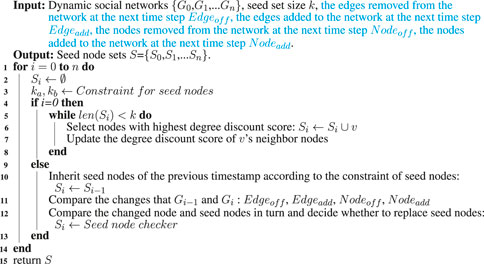
In Algorithm 2, we impose constraints on the categories of seed nodes. Here, $V_i(a)$ represents the set of nodes with category ’a’ at time $i$. $nod{e}_a$ and $nod{e}_b$ represent sets of nodes with categories ’a’ and ’b’, respectively. The algorithm first traverses all nodes in the graph and calculates the counts of nodes for each category. Then, based on their proportions in the network, it determines the proportions of the two categories of nodes in the seed node set. Additionally, we dynamically update the seed node set according to the changes in the social network.

The seed checker plays a crucial role in the seed node selection strategy. Its function is to compare the degree discount scores between the changing node and the previous timestamp’s seed nodes. Then, it decides whether to replace the previous seed nodes with the changing node. We provide a detailed description of this process in Algorithm 3. The input consists of the current network, the set of seed nodes to be updated, the node $u$ to be checked, and its degree discount score. The output is the updated set of seed nodes. Here, $S_i(a)$ represents the set of nodes with category ’a’ in the seed node set at the $i$-th timestamp. Due to the limitation on node categories, we first determine the category of the changing node $u$. Then, we compare node $u$ with seed nodes of the same category. If the degree discount score of $u$ is greater than that of any seed node, we replace the seed node with the lowest degree discount score with $u$.

Algorithm 3

Algorithm 3. Procedure of the seed checker.

Based on Algorithm 2 and Algorithm 3, we propose the SSHD. We combine the seed nodes from the previous timestamp with the changed nodes to obtain the seed node set for the current timestamp. Through continuous iteration, we can obtain the seed node set corresponding to each timestamp. Due to the smooth changes in the network structure, within a small time interval, the network topology does not undergo drastic changes. Therefore, we only need to focus on the changed nodes without involving all nodes. We recalculate the degree discount scores based on the changed nodes according to Algorithm 1. Finally, by comparing the degree discount scores of the seed nodes selected at the previous timestamp with those of the changed nodes, we update the seed node set for the current timestamp.

Algorithm 4

Algorithm 4. Seed nodes selection strategy considering homophily and dynamics.

Algorithm 4 presents the overall framework of SSHD. The input includes the dynamic social network graph and the number of seed nodes. The output is the corresponding seed node set. When $i$ equals 0, we select seed nodes on the initial social network. Under the constraint of seed node category, we choose the node with the highest degree discount score as the seed node. The operation of updating node degree discount scores is shown in Algorithm 1. As the network evolves, we need to update the seed set accordingly. In step 7, we allocate the seed nodes from the previous timestamp to the current timestamp. However, this is not just a simple allocation operation; it implies the constraint of seed node category. If the seed node category constraints of two timestamps are different, we will randomly select non-seed nodes from the network to fill the blank space in $S_i$. Step 8 is to compare the changes that occur in the social network. We can obtain a set of disappearing edges (nodes whose edges have not changed), a set of new edges (nodes whose edges have not changed), a set of disappearing nodes, and a set of new nodes. In step 9, we compare the degree discount scores of existing seed nodes and changed nodes. The changed nodes are all nodes related to the sets obtained in step 8. We recalculate their degree discount scores using Algorithm 1. The replacement operation is performed by the seed checker.

4.4 Independent cascade model based on influence homophily and dynamics

Kempe et al. [12] proposed the traditional independent cascade model, where the probability parameter of an edge determines whether a node will activate its neighboring nodes. However, McPherson et al. [36] demonstrated that homophily is widespread in social networks. For example, if two people simultaneously recommend products to a user, the user is more likely to be influenced by people with similar attributes. These attributes can include gender, interests, status, etc. The traditional independent cascade model only considers the position of nodes in the social network without taking into account node features. In other words, previous studies typically determine whether one node will influence another based on network topology without considering homophily in social networks. Based on this observation, we propose the ICIHD. In the ICIHD, the centrality of nodes determines the initial probability parameter of edges. Then, we combine homophily with centrality measures as the probability parameter of edges between nodes. The inherent implication of homophily is to appropriately increase the probability of influence between two users with the same attributes. The role of the influence propagation model is to output the set of nodes activated by seed nodes. As the seed node set is continuously updated over time, the set of activated nodes also changes accordingly.

4.4.1 Centrality measurement methods

Centrality can measure the influence of nodes in a network. We define the initial edge probability parameters by evaluating the centrality of nodes on both sides of the edge. Specifically, the probability formula for one node activating another node is as follows:

$p\left(u,v\right)=\frac{C\left(u\right)}{C\left(u\right)+C\left(v\right)}(9)$

Where $p(u,v)$ is the probability of node $u$ activating node $v$, and $C(u)$ is the centrality of node $u$. In a directed graph, influence can only propagate from one node to the node it points to. Therefore, defining the probability parameters in this way can effectively simulate the probability of edges. In the special case where both nodes $u$ and $v$ have centrality of 0, influence cannot propagate through this edge.Although node centrality can estimate the probability of influence propagation, in online social networks, the propagation probability between nodes is usually not very high [37]. To more accurately simulate the influence propagation process in online social networks and make the edge probability parameters derived from centrality closer to real values in online social networks, we introduce a correction factor $\lambda$ in Equation 9 to adjust the propagation probability, as shown in Equation 10.

$p\left(u,v\right)=\frac{\lambda C\left(u\right)}{C\left(u\right)+C\left(v\right)}(10)$

To avoid the impact of a single centrality measure on the experimental results, we employed four different node centrality measurement methods and evaluated the performance of different types of centrality measurement methods. They are degree centrality [38], eccentric centrality [39], PageRank centrality [40], and closeness centrality [41]. These four centrality measurement methods are based on different node attributes and positions, covering several fundamental types of methods. Therefore, they can represent general centrality measurement methods.

4.4.2 Edge probability parameters evaluation method

In this subsection, we propose a method for evaluating edge probability parameters considering influence homophily, formulated as follows:

$EP\left(u,v\right)=\alpha p\left(u,v\right)+\left(1-\alpha \right)h_p\left(u,v\right)(11)$

$h_p\left(u,v\right)=\left\{\begin{array}{cc}{h}_p\hfill & u\text{\hspace{0.17em}and\hspace{0.17em}}v\text{\hspace{0.17em}belong\hspace{0.17em}to\hspace{0.17em}the\hspace{0.17em}same\hspace{0.17em}category}\hfill \\ \lambda -h_p\hfill & \text{otherwise}\hfill \end{array}\right.(12)$

Where $EP(u,v)$ represents the probability of node $u$ influencing node $v$. $p(u,v)$ is the initial edge parameter mentioned earlier, computed using the four different methods for calculating node centrality described previously. $h_p$ is the influence homophily parameter, which needs to be of the same order of magnitude as $p(u,v)$. Since edge parameters belong to the (0, 1) interval, we use a trade-off coefficient $\alpha$. We will validate the different performance reflected by different $\alpha$ and different $h_p$ in the experiments.

4.4.3 Influence propagation process

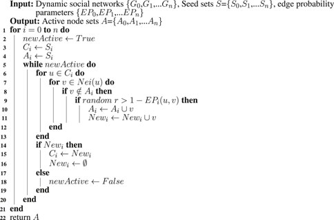
The process of influence propagation in the independent cascade model is as follows: An activated node attempts to activate its neighboring nodes with a certain probability. This activation attempt occurs only once, and the attempts of different nodes are independent of each other. The newly activated nodes continue to attempt to activate their neighboring nodes. This process continues until there are no new activated nodes in the network. Due to the dynamic nature of social networks, the edge parameters between nodes and the results of influence diffusion will also change accordingly.

Algorithm 5

Algorithm 5. The process of influence propagation.

In Algorithm 5, we describe the process of influence propagation given a seed node set in dynamic social networks. The input consists of the dynamic social network, the corresponding seed node set, and the set of edge probability parameters. The output is the active node set corresponding to each timestamp. Here, $newActive$ is an indicator. If the indicator is true, there are new active nodes in the network. When the indicator is false, the influence propagation process terminates. $C_i$ represents the current set of active nodes. $Nei(u)$ represents the neighbor nodes of node $u$. $Ne{w}_i$ is the set of currently activated nodes. Steps 6–13 demonstrate the process where current active nodes attempt to activate their adjacent nodes. The random number $r$ belongs to the range 0–1. The edge probability parameters between nodes $u$ and $v$ determine the likelihood of node $u$ activating node $v$. If the edge probability parameter is higher, node $u$ is more likely to activate node $v$. Steps 14–19 involve checking for any new active nodes.

5 Experiments

In this section, we conduct three experiments to evaluate the performance of SSHD. The first experiment analyzes the performance of SSHD under different parameter settings. The second experiment compares SSHD with other baseline methods in static social networks. In the third experiment, we evaluate the continuity performance of SSHD in dynamic social networks and compare it with other baseline methods. The following subsections present the experimental details and discuss the results.

5.1 Datasets

We selected the professional Twitter accounts of four major companies: Bank of America, UPS, Verizon, and Hershey, which frequently post job advertisements. Using the Twitter API, we obtained the followers of each account to form a complete social network, including followers of followers, based on the follower connections. Due to limited information available in the dataset, we categorized users into two categories based on their gender. The gender of users was determined by the Genderize API using their names. The Genderize API utilizes a vast database containing names from different countries and languages along with their associated genders. Karimi et al. [42] demonstrated the high accuracy of this database. We defined male users in these four datasets as category ’a’, comprising the majority, while female users were categorized as category ’b’, representing the minority. The homophily index of the network is proportional to the ratio of edges connecting two nodes of the same category. Table 1 provides detailed information about the aforementioned four datasets.

Table 1

Table 1. Details of the datasets.

M.S. et al. [23] proposed a homophily network generation model. To simulate the dynamic evolution of the network, we utilized this model to process the hersheycareers dataset. The network evolves over time as follows: 1) At timestamp 1: 4,035 nodes and 24,877 edges. 2) At timestamp 2: 4,163 nodes and 25,184 edges. 3) At timestamp 3: 4,529 nodes and 26,237 edges. 4) At timestamp 4: 5,168 nodes and 28,551 edges.

5.2 Baseline methods

$•$ Degree Discount [16]: This algorithm improves upon degree-based heuristic algorithms. Whenever a node becomes a seed node, the algorithm updates its neighboring nodes using Equation 8.

$•$ CELF [13]: CELF further improves upon greedy algorithms by exploiting submodularity properties. It is more efficient than general greedy algorithms and also provides certain performance guarantees.

$•$ BalGreedy [23]: The core of BalGreedy is a greedy approach. It calculates the marginal gain of nodes using Equation 13. This equation tends to select fewer nodes after selecting the majority of nodes to promote balance in the proportion of nodes in the final set of active nodes.

$F\left(S\right)=\underset{\text{Influence\hspace{0.17em}}}{\underbrace{\left(1-\lambda \right)\cdot \frac{f\left(S\right)}{|V|}}}+\underset{\text{Balance\hspace{0.17em}}}{\underbrace{\lambda \cdot \frac{\sqrt{\gamma M\left(S\right)}+\sqrt{\left(1-\gamma \right)m\left(S\right)}}{\sqrt{\gamma p_{M}n}+\sqrt{\left(1-\gamma \right)\left(1-p_M\right)n}}}}(13)$

$•$ BalDegree [43]: BalDegree selects seed nodes based on their degree, but it does not simply choose the nodes with the highest degree from the entire network. Instead, it selects the nodes with the highest degree from each group.

$•$ ABEM [27]: ABEM is an adaptive agent-based evolutionary method for finding seed nodes. The algorithm utilizes an adaptive optimizer to drive the evolutionary process and dynamically adjust candidate solutions.

5.3 Experimental results and discussion

As mentioned earlier, our goal is not only to maximize influence by reaching a sufficient number of nodes but also to strive for a proportion of influenced nodes that closely resembles the proportion in the initial network. In the experimental results, we should not only consider the size of the influenced range but also pay attention to the balance of influence. To measure influence balance, we define a metric as the difference between the product of the number of active nodes and the proportion of category ’a’ nodes in the initial network, and the actual number of category ’a’ nodes activated. In other words, the closer the difference is to zero, the better the effect. A larger difference indicates a higher level of imbalance. Perfect influence balance would mean achieving a difference of zero. Considering the stochastic nature of influence diffusion in experiments, we take the average of 100 experimental results as the observation metric. To prevent positive and negative values from canceling each other out in the difference, the calculated difference is absolute-valued.

5.3.1 Experiment 1: performance of SSHD under different parameter settings

First, we compare the effects of the influence maximization algorithm under different homophily parameters. In this experiment, we set $\lambda$ = 0.01, $\alpha$ = 0.5, and use the degree centrality measurement method. The impact of these parameters on the experimental results is also be discussed later. In online social networks, the probability of influence propagation between nodes of the same category should be higher than that between nodes of different categories [23]. Therefore, based on Equations 11, 12, we set the value of the homophily parameter $h_p$ to (0.005, 0.006, 0.007, 0.008, 0.009, 0.01). The diffusion results are shown in Figure 4, and the balance effect is shown in Figure 5.

Figure 4

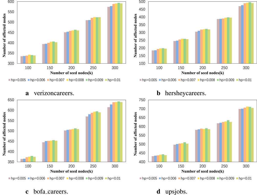
Figure 4. (A) verizoncareers. (B) hersheycareers. (C) bofa_careers. (D) upsjobs. The influence range results of our algorithm when using different homophily parameters.

Figure 5

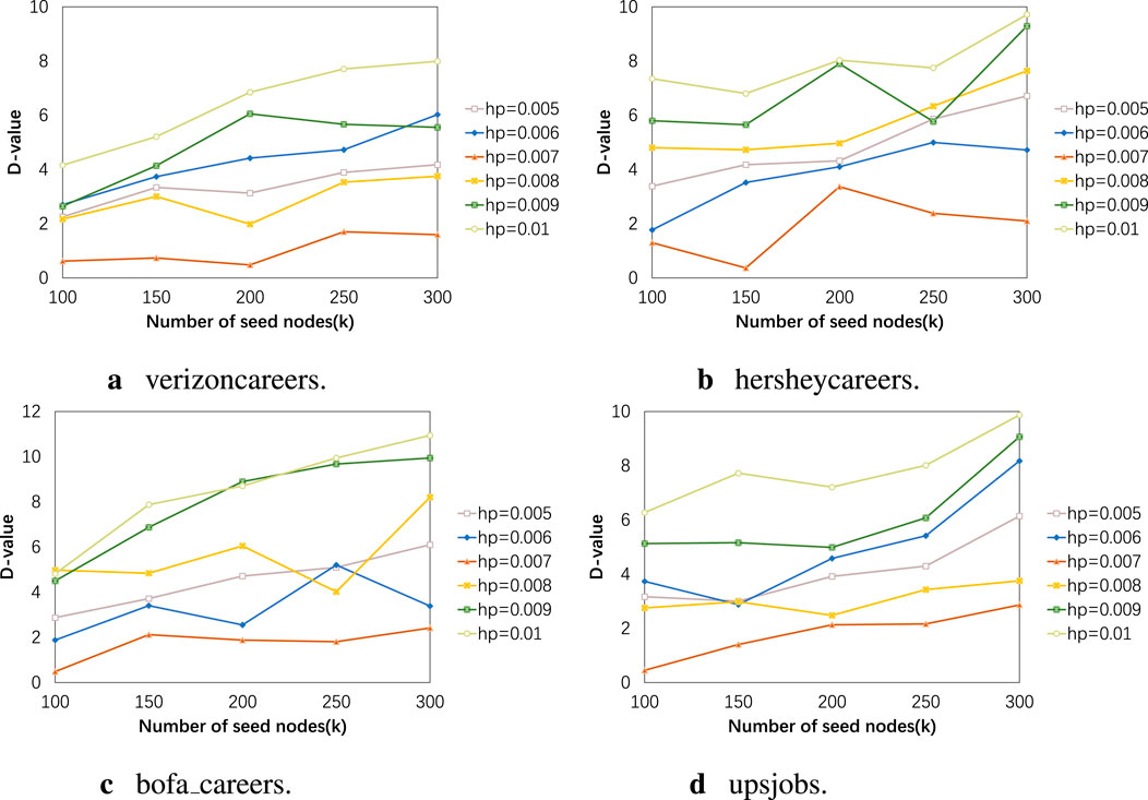
Figure 5. (A) verizoncareers. (B) hersheycareers. (C) bofa_careers. (D) upsjobs. The influence balance results of our algorithm when using different homophily parameters.

In Figure 4, the vertical axis represents the number of active nodes, with the upward bars indicating a wider range of influence. In Figure 5, the vertical axis represents the absolute difference between the product of the number of active nodes and the proportion of category ’a’ nodes in the initial network and the actual number of activated category ’a’ nodes. A lower value indicates a better balance effect. Their horizontal axes correspond to different sizes of seed node sets. The results in Figures 4, 5 correspond one-to-one. It can be seen that when the homophily parameter is set to 0.007, good results are obtained in both influence range and balance effect, regardless of the dataset. For example, in the experiment results of the bofa_careers dataset with a homophily parameter of 0.007, the maximum influence range is 638.9 nodes, which is only 3.9 nodes less than when the homophily parameter is 0.009. However, in terms of balance effect, the former differs from perfect balance by 2.4 nodes, while the latter differs by 9.9 nodes. Due to the averaging of 100 experimental data points, decimal values may appear in the experimental results. This may be because the role of the homophily parameter in the experiment is to appropriately increase the probability of influence between nodes with the same attributes. This increase in probability needs to be moderate, as nodes with the same attributes may be more likely to influence each other, but this does not mean that influence between nodes with different attributes will not propagate. In Figures 6, 7, we discuss the different effects of different weights. Similar to the previous experiment, we use the degree centrality measurement method and set the homophily index to 0.007. Node centrality and node features jointly determine the propagation probability of edges. This weight represents the proportion of node centrality, and it is set to (0.4, 0.5, 0.6, 0.7). From the experimental results, it can be observed that regardless of the data scale, a weight of 0.5 can achieve the ideal effect, meaning that the influence range is sufficiently large and the influence is relatively balanced. Additionally, the higher the homophily index in the network, the worse the balance effect. For example, the network structure homophily index of the upsjobs dataset is much larger than that of the other three datasets, so the gap between the results of the upsjobs dataset and the x-axis is larger.

Figure 6

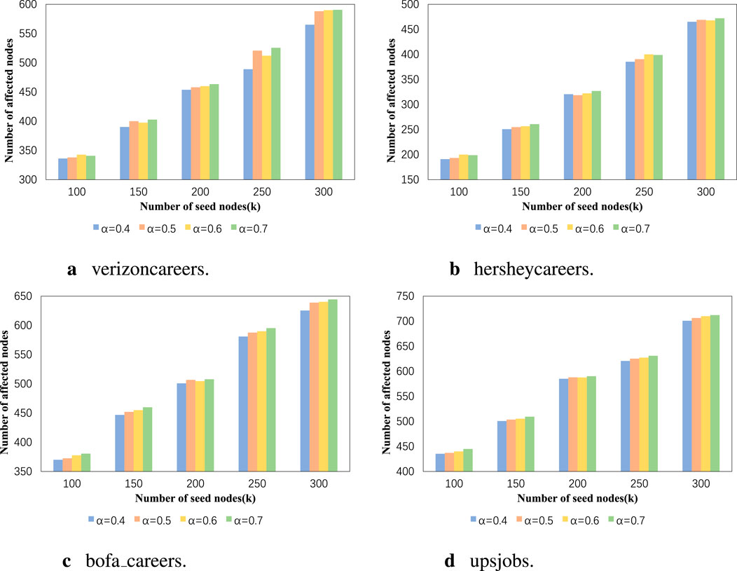
Figure 6. (A) verizoncareers. (B) hersheycareers. (C) bofa_careers. (D) upsjobs. The influence range results of our algorithm when using different weights.

Figure 7

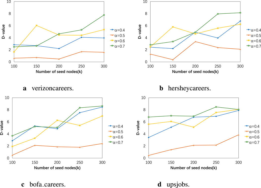
Figure 7. (A) verizoncareers. (B) hersheycareers. (C) bofa_careers. (D) upsjobs. The influence balance results of our algorithm when using different weights.

Next, we test the effectiveness of using different centrality measurement methods in terms of influence range and influence balance. We use degree centrality measurement method, PageRank centrality measurement method, closeness centrality measurement method, and eccentricity centrality measurement method. In this experiment, the weight $\alpha$ is set to 0.5, and the homophily parameter is set to 0.007. The experimental results are shown in Figures 8, 9. The results show that degree centrality measurement method outperforms the other three methods in both influence range and influence balance. It is based on the number of connections a node has with other nodes. Among the four datasets, the eccentricity centrality measurement method performs the worst. This may be because eccentricity centrality depends only on the distance to the network center, without considering the relationships between nodes and the network structure.

Figure 8

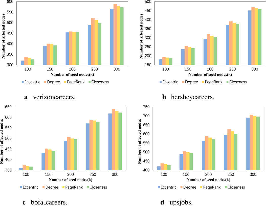
Figure 8. (A) verizoncareers. (B) hersheycareers. (C) bofa_careers. (D) upsjobs. The influence range results of our algorithm when using different centrality measurement methods.

Figure 9

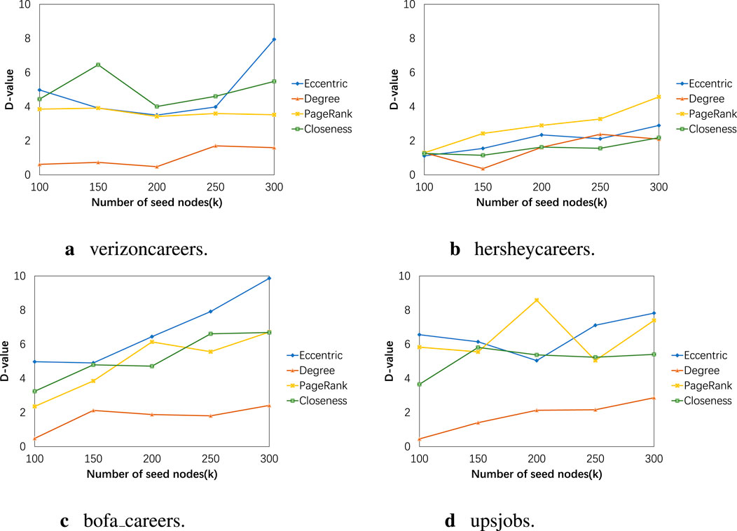
Figure 9. (A) verizoncareers. (B) hersheycareers. (C) bofa_careers. (D) upsjobs. The influence balance results of our algorithm when using different centrality measurement methods.

5.3.2 Experiment 2: Comparison of SSHD and baseline methods on static social networks

Based on the results of Experiment 1, we set the weight $\alpha$ in the influence propagation model to 0.5 and the homophily parameter to 0.007. By using the degree centrality measurement method, we compare the proposed algorithm with other benchmark methods on four networks with different data scales and network structure homophily parameters. The experimental results are shown in Figures 10, 11. The SSHD algorithm, BalGreedy algorithm, and BalDegree algorithm all employ certain methods to promote influence balance. Therefore, in the experimental results in Figure 11, the seed nodes selected by the degree discount algorithm and the CELF algorithm result in significant imbalance. In Figure 10, the BalGreedy algorithm and the CELF algorithm achieve better influence range, while BalDegree performs the worst. This is because BalGreedy and CELF use greedy algorithms, which are more accurate than the other three heuristic algorithms. The degree discount algorithm and the SSHD algorithm not only select seed nodes based on node degrees but also discount the degree scores of their neighboring nodes after determining the seed nodes. From the experimental results, it can be seen that regardless of the dataset, the SSHD algorithm is significantly better than other algorithms in terms of influence balance. Furthermore, our proposed algorithm only makes a slight sacrifice in influence range. Since the network structure homophily index of the upsjobs dataset is much larger than that of the other three datasets, using traditional algorithms on the upsjobs dataset may result in severe imbalance. Therefore, our SSHD algorithm is preferred when the homophily index of the network structure is large, as it balances influence range and influence balance.

Figure 10

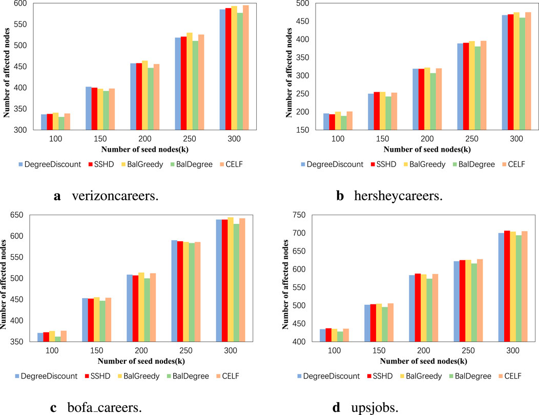
Figure 10. (A) verizoncareers. (B) hersheycareers. (C) bofa_careers. (D) upsjobs. The influence range results on four datasets using five different algorithms.

Figure 11

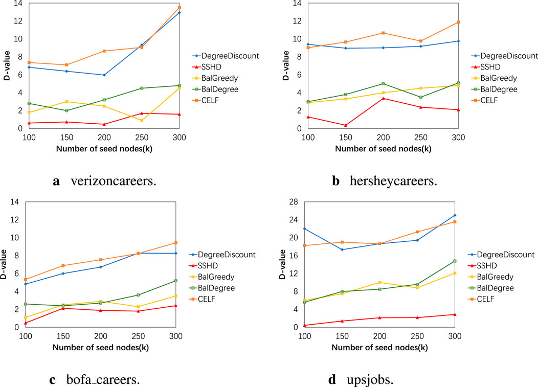
Figure 11. (A) verizoncareers. (B) hersheycareers. (C) bofa_careers. (D) upsjobs. The influence balance results on four datasets using five different algorithms.

Additionally, we compare the running times of these five algorithms. Similarly, we use the average results of 100 experiments as the observation indicators. The results are shown in Table 2. Since the SSHD, BalDegree, and degree discount algorithms are heuristic algorithms, their running times are much shorter than the other two algorithms. The running time of the algorithms is also proportional to the size of the dataset.

Table 2

Table 2. Average running times of different algorithms in different experimental datasets (Unit of measurement: seconds).

5.3.3 Experiment 3: comparison of SSHD and baseline methods on dynamic social networks

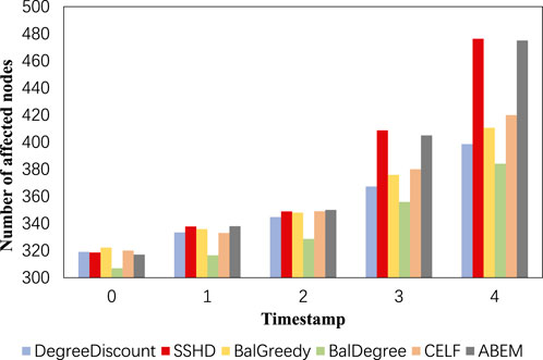
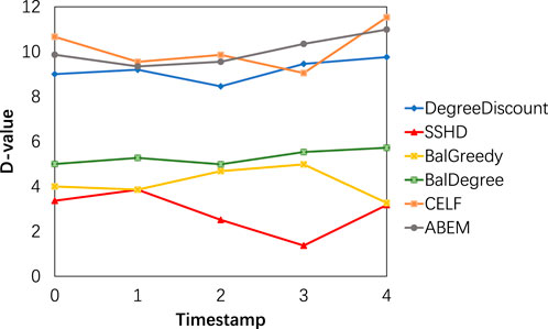
In this experiment, we validate the performance of the proposed algorithm on dynamic social networks. In the above experiments, the results with different numbers of seed nodes are similar, so we choose to conduct experiments with $k=200$. Additionally, we set $h_p=0.007$, $\alpha =0.5$, and use the degree centrality method. Figures 12, 13 show the influence range and influence balance, respectively. The horizontal axis represents the timestamp. As the timestamp changes, the topology of the network also changes. The specific details are described in section 5.1. It can be seen that at timestamps 1 and 2, the influence range of SSHD and ABEM is very close to that of the BalGreedy and CELF algorithms. However, at timestamps three and 4, the influence range of SSHD and ABEM is much larger than the other four algorithms. This is because the network topology undergoes significant changes later on. SSHD and ABEM are able to update the seed node set in a timely manner based on changes in the network topology. In terms of influence balance, despite the dynamic changes in the network, our SSHD algorithm still outperforms the other five algorithms.

Figure 12

Figure 12. The influence range results on dynamic hersheycareers dataset.

Figure 13

Figure 13. The influence balance results on dynamic hersheycareers dataset.

6 Conclusion

In this study, we proposed a homophilic and dynamic influence maximization strategy based on independent cascade model. Specifically, HDIM consists of two parts: SSHD and ICIHD. Through in-depth analysis of node attributes and connection patterns in social networks, we designed the SSHD strategy to more accurately select seed nodes and effectively evaluate the degree discount scores of nodes through the DDD heuristic strategy. At the same time, we proposed the ICIHD model, which redefines the propagation probability between nodes to fully consider the impact of homophily parameters and network dynamics on the propagation process. Our experimental results show that the proposed method achieves good performance on multiple static and dynamic social network datasets. Compared with traditional methods, our method can more effectively activate nodes and better maintain the proportion of node types in the initial network. In dynamic social networks, our method is more adaptive and can more accurately respond to changes in network structure.

In summary, this study provides a new perspective and method for solving the influence maximization problem in social networks. Our work is of great significance for understanding the regularity and mechanism of information propagation in social networks, and provides valuable reference for promotion and implementation in practical applications. In future research, we will further explore more complex network models and algorithms to cope with the diversity and dynamics of social networks, while also conducting a detailed complexity analysis to assess their scalability and efficiency.

Data availability statement

The datasets presented in this study can be found in online repositories. The names of the repository/repositories and accession number(s) can be found in the article/supplementary material.

Author contributions

GW: Conceptualization, Methodology, Writing–original draft. SD: Investigation, Methodology, Software, Writing–original draft. YJ: Validation, Visualization, Writing–review and editing. XL: Writing–review and editing.

Funding

The author(s) declare that financial support was received for the research, authorship, and/or publication of this article. This research was funded by the National Natural Science Foundation of China (Grant Nos. 61872298, 61802316, and 61902324), the Sichuan Science and Technology Program (Grant No. 2023YFQ0044).

Conflict of interest

The authors declare that the research was conducted in the absence of any commercial or financial relationships that could be construed as a potential conflict of interest.

Generative AI statement

The author(s) declare that no Generative AI was used in the creation of this manuscript.

Publisher’s note

All claims expressed in this article are solely those of the authors and do not necessarily represent those of their affiliated organizations, or those of the publisher, the editors and the reviewers. Any product that may be evaluated in this article, or claim that may be made by its manufacturer, is not guaranteed or endorsed by the publisher.

References

1. Li S, Jiang L, Wu X, Han W, Zhao D, Wang Z. A weighted network community detection algorithm based on deep learning. Appl Math Comput (2021) 401:126012. doi:10.1016/j.amc.2021.126012

CrossRef Full Text | Google Scholar

2. Du Y, Zhou Q, Luo J, Li X, Hu J. Detection of key figures in social networks by combining harmonic modularity with community structure-regulated network embedding. Inf Sci (2021) 570:722–43. doi:10.1016/J.INS.2021.04.081

CrossRef Full Text | Google Scholar

3. Gong M, Yan J, Shen B, Ma L, Cai Q. Influence maximization in social networks based on discrete particle swarm optimization. Inf Sci (2016) 367:600–14. doi:10.1016/j.ins.2016.07.012

CrossRef Full Text | Google Scholar

4. Currarini S, Jackson MO, Pin P. Identifying the roles of race-based choice and chance in high school friendship network formation. PNAS (2010) 107:4857–61. doi:10.1073/pnas.0911793107

PubMed Abstract | CrossRef Full Text | Google Scholar

5. Kumar S, Mallik A, Panda B. Influence maximization in social networks using transfer learning via graph-based lstm. Expert Syst Appl (2023) 212:118770. doi:10.1016/j.eswa.2022.118770

CrossRef Full Text | Google Scholar

6. Cheng J, Yang K, Yang Z, Zhang H, Zhang W, Chen X. Influence maximization based on community structure and second-hop neighborhoods. Appl Intell (2022) 52:10829–44. doi:10.1007/s10489-021-02880-8

CrossRef Full Text | Google Scholar

7. Gong C, Du Y, Li X, Chen X, Li X, Wang Y, et al. Structural hole-based approach to control public opinion in a social network. Eng Appl Artif Intell (2020) 93:103690. doi:10.1016/j.engappai.2020.103690

CrossRef Full Text | Google Scholar

8. Huang H, Meng Z, Shen H. Competitive and complementary influence maximization in social network: a follower’s perspective. Knowledge-based Syst (2021) 213:106600. doi:10.1016/j.knosys.2020.106600

CrossRef Full Text | Google Scholar

9. Zhuang H, Sun Y, Tang J, Zhang J, Sun X. Influence maximization in dynamic social networks. In: 2013 IEEE 13th international conference on data mining. Dallas, TX, USA: IEEE Computer Society (2013) p. 1313–8. doi:10.1109/ICDM.2013.145

CrossRef Full Text | Google Scholar

10. Barabási AL, Albert R. Emergence of scaling in random networks. science (1999) 286:509–12. doi:10.1126/science.286.5439.509

PubMed Abstract | CrossRef Full Text | Google Scholar

11. Domingos P, Richardson M. Mining the network value of customers. In: Seventh ACM SIGKDD international conference on knowledge discovery and data mining. New York, NY, USA (2001). p. 57–66. doi:10.1145/502512.502525

CrossRef Full Text | Google Scholar

12. Kempe D, Kleinberg J, Tardos É. Maximizing the spread of influence through a social network. In: Ninth ACM SIGKDD international conference on Knowledge discovery and data mining. New York, NY, USA (2003) p. 137–46. doi:10.4086/toc.2015.v011a004

CrossRef Full Text | Google Scholar

13. Leskovec J, Krause A, Guestrin C, Faloutsos C, VanBriesen J, Glance N. Cost-effective outbreak detection in networks. In: 13th ACM SIGKDD international conference on Knowledge discovery and data mining. New York, NY, USA (2007) p. 420–9. doi:10.1145/1281192.1281239

CrossRef Full Text | Google Scholar

14. Heidari M, Asadpour M, Faili H. Smg: fast scalable greedy algorithm for influence maximization in social networks. Phys A: Stat Mech Appl (2015) 420:124–33. doi:10.1016/j.physa.2014.10.088

CrossRef Full Text | Google Scholar

15. Chen W, Peng B, Schoenebeck G, Tao B. Adaptive greedy versus non-adaptive greedy for influence maximization. J Artif Intell Res (2022) 74:303–51. doi:10.1613/jair.1.12997

CrossRef Full Text | Google Scholar

16. Chen W, Wang Y, Yang S. Efficient influence maximization in social networks. In: 15th ACM SIGKDD international conference on Knowledge discovery and data mining. New York, NY, USA (2009). p. 199–208. doi:10.1145/1557019.1557047

CrossRef Full Text | Google Scholar

17. Zhang B, Wang Y, Jin Q, Ma J. A pagerank-inspired heuristic scheme for influence maximization in social networks. Int J Web Serv Res (2015) 12:48–62. doi:10.4018/IJWSR.2015100104

CrossRef Full Text | Google Scholar

18. Jia W, Yan L, Ma Z, Niu W. Tph: a three-phase-based heuristic algorithm for influence maximization in social networks. J Intell Fuzzy Syst (2020) 39:4393–403. doi:10.3233/JIFS-200383

CrossRef Full Text | Google Scholar

19. Kossinets G, Watts DJ. Origins of homophily in an evolving social network. Am J Sociol (2009) 115:405–50. doi:10.1086/599247

CrossRef Full Text | Google Scholar

20. Aral S, Muchnik L, Sundararajan A. Engineering social contagions: optimal network seeding in the presence of homophily. Netw Sci (2013) 1:125–53. doi:10.1017/nws.2013.6

CrossRef Full Text | Google Scholar

21. Xie X, Li J, Sheng Y, Wang W, Yang W. Competitive influence maximization considering inactive nodes and community homophily. Knowledge-based Syst (2021) 233:107497. doi:10.1016/j.knosys.2021.107497

CrossRef Full Text | Google Scholar

22. Chen YC, Zhu WY, Peng WC, Lee WC, Lee SY. Cim: community-based influence maximization in social networks. ACM Trans Intell Syst Technol (2014) 5(25):1–31. doi:10.1145/2532549

CrossRef Full Text | Google Scholar

23. Anwar MS, Saveski M, Roy D. Balanced influence maximization in the presence of homophily. In: Fourteenth ACM international conference on web search and data mining. Israel: Virtual Event (2021) p. 175–83. doi:10.1145/3437963.3441787

CrossRef Full Text | Google Scholar

24. Sheng W, Song W, Li D, Yang F, Zhang Y. Dynamic influence maximization via network representation learning. Front Phys (2021) 9:827468. doi:10.3389/fphy.2021.827468

CrossRef Full Text | Google Scholar

25. Song G, Li Y, Chen X, He X, Tang J. Influential node tracking on dynamic social network: an interchange greedy approach. IEEE Trans Knowl Data Eng (2016) 29:359–72. doi:10.1109/TKDE.2016.2620141

CrossRef Full Text | Google Scholar

26. Zhang L, Li K. Influence maximization based on snapshot prediction in dynamic online social networks. Mathematics (2022) 10:1341. doi:10.3390/math10081341

CrossRef Full Text | Google Scholar

27. Li W, Hu Y, Jiang C, Wu S, Bai Q, Lai E. ABEM: an adaptive agent-based evolutionary approach for influence maximization in dynamic social networks. Appl Soft Comput (2023) 136:110062. doi:10.1016/j.asoc.2023.110062

CrossRef Full Text | Google Scholar

28. Chandran J, Viswanatham VM. Dynamic node influence tracking based influence maximization on dynamic social networks. Microprocess Microsyst (2022) 95:104689. doi:10.1016/j.micpro.2022.104689

CrossRef Full Text | Google Scholar

29. Jendoubi S, Martin A, Liétard L, Hadji HB, Yaghlane BB. Two evidential data based models for influence maximization in twitter. Knowl Based Syst (2017) 121:58–70. doi:10.1016/j.knosys.2017.01.014

CrossRef Full Text | Google Scholar

30. Wang Z, Chen X, Li X, Du Y, Lan X. Influence maximization based on network representation learning in social network. Intell Data Anal (2022) 26:1321–40. doi:10.3233/IDA-216149

CrossRef Full Text | Google Scholar

31. Li L, Liu Y, Zhou Q, Yang W, Yuan J. Targeted influence maximization under a multifactor-based information propagation model. Inf Sci (2020) 519:124–40. doi:10.1016/j.ins.2020.01.040

CrossRef Full Text | Google Scholar

32. Bozorgi A, Samet S, Kwisthout J, Wareham T. Community-based influence maximization in social networks under a competitive linear threshold model. Knowl Based Syst (2017) 134:149–58. doi:10.1016/j.knosys.2017.07.029

CrossRef Full Text | Google Scholar

33. Li W, Li Z, Luvembe AM, Yang C. Influence maximization algorithm based on Gaussian propagation model. Inf Sci (2021) 568:386–402. doi:10.1016/j.ins.2021.04.061

CrossRef Full Text | Google Scholar

34. Guo C, Li W, Liu F, Zhong K, Wu X, Zhao Y, et al. Influence maximization algorithm based on group trust and local topology structure. Neurocomputing (2024) 564:126936. doi:10.1016/j.neucom.2023.126936

CrossRef Full Text | Google Scholar

35. Yang S, Du Q, Zhu G, Cao J, Chen L, Qin W, et al. Balanced influence maximization in social networks based on deep reinforcement learning. Neural Networks (2024) 169:334–51. doi:10.1016/j.neunet.2023.10.030

PubMed Abstract | CrossRef Full Text | Google Scholar

36. McPherson M, Smith-Lovin L, Cook JM. Birds of a feather: homophily in social networks. Annu Rev Sociol (2001) 27:415–44. doi:10.1146/annurev.soc.27.1.415

CrossRef Full Text | Google Scholar

37. Deng X, Dou Y, Lv T, Nguyen QVH. A novel centrality cascading based edge parameter evaluation method for robust influence maximization. IEEE Access (2017) 5:22119–31. doi:10.1109/ACCESS.2017.2764750

CrossRef Full Text | Google Scholar

38. Jia P, Liu J, Huang C, Liu L, Xu C. An improvement method for degree and its extending centralities in directed networks. Phys A: Stat Mech Appl (2019) 532:121891. doi:10.1016/j.physa.2019.121891

CrossRef Full Text | Google Scholar

39. Kenett DY, Perc M, Boccaletti S. Networks of networks–an introduction. Chaos Solit Fractals (2015) 80:1–6. doi:10.1016/j.chaos.2015.03.016

CrossRef Full Text | Google Scholar

40. Lv L, Zhang K, Zhang T, Bardou D, Zhang J, Cai Y. Pagerank centrality for temporal networks. Phys Lett A (2019) 383:1215–22. doi:10.1016/j.physleta.2019.01.041

CrossRef Full Text | Google Scholar

41. Kim JY. Information diffusion and closeness centrality. Sociol Theor Methods (2010) 25:95–106. doi:10.11218/ojjams.25.95

CrossRef Full Text | Google Scholar

42. Karimi F, Wagner C, Lemmerich F, Jadidi M, Strohmaier M. Inferring gender from names on the web: a comparative evaluation of gender detection methods. In: 25th International conference companion on world wide web (republic and canton of Geneva, CHE) (2016) p. 53–4. doi:10.1145/2872518.2889385

CrossRef Full Text | Google Scholar

43. Stoica AA, Han JX, Chaintreau A. Seeding network influence in biased networks and the benefits of diversity. In: Web conference 2020. New York, NY, USA (2020) p. 2089–98. doi:10.1145/3366423.3380275

CrossRef Full Text | Google Scholar