Self-organization of the stock exchange to the edge of a phase transition: empirical and theoretical studies

Our study is based on the hypothesis that stock exchanges, being nonlinear, open and dissipative systems, are capable of self-organization to the edge of a phase transition. To empirically support the hypothesis, we find segments in hourly stock volume series for 3,000 stocks of publicly traded companies, corresponding to the time of stock exchange’s stay to the edge of a phase transition. We provide a theoretical justification of the hypothesis and present a phenomenological model of stock exchange self-organization to the edge of the first-order phase transition and to the edge of the second-order phase transition. In the model, the controlling parameter is entropy as a measure of uncertainty of information about a share of a public company, guided by which stock exchange players make a decision to buy/sell it. The order parameter is determined by the number of buy/sell transactions by stock exchange players of a public company’s shares, i.e., stock’s volume. By applying statistical tests and the AUC metric, we found the most effective early warning measures from the set of investigated critical deceleration measures, multifractal measures and reconstructed phase space measures. The practical significance of our study is determined by the possibility of early warning of self-organization of stock exchanges to the edge of a phase transition and can be extended with high frequency data in the future research.

1 Introduction

More than 35 years ago, P. Bak together with C. Tang suggested that in nonlinear systems far from equilibrium, complex holistic properties may emerge through their self-organization into a critical state [1]. Subsequently, the theory of self-organized criticality (SOC) was formed, the main provisions of which have found application in sociology, biological evolution, seismology, economics and other sciences (e.g., see the papers [2–7, 7–9]). The theory of self-organization at the edge of phase transitions has found applications in cognitive and social science (e.g., see the papers [10, 11]).

The basic model of SOC theory is the sandpile cellular automaton (SCA), which demonstrates how complex holistic properties emerge in a model system with simple rules as a result of self-organization of the automaton into a critical state (e.g., see the papers [12, 13]). The simplest model of SCA is the following model. Suppose that the nodes of the lattice graph are assigned integer numbers (the number of grains of sand in the cells). Then we increase by one the numbers assigned to randomly chosen nodes of the graph (add one grain of sand in the cells). If the number (grains of sand), $z_{k,l}$, for some node $\left(k,l\right)$ exceeds some threshold value, $z_c$, for instance $z_c=4$, then this node is unstable and its toppling occurs. As a result of node toppling $\left(k,l\right)$ numbers for neighbouring nodes, $z_{k\pm 1,l\pm 1}$, are increased by 1, i.e., $z_{k\pm 1,l\pm 1}\to z_{k\pm 1,l\pm 1}+4$. Thus $z_{k,l}\to z_{k,l}-4$. Collapses occur until the SCA becomes stable, that is, until at each node $z_{k,l}<4$.

Each iteration of the SCA simulation is followed by its perturbation, by adding one grain of sand to randomly selected cells at a time, and relaxation, by collapsing unstable cells. Starting from some critical iteration, $i_c$, a single added grain of sand in a randomly selected cell can cause an avalanche of collapses of any size, continuing until all cells regain stability. In the subcritical phase ($i<i_c$) avalanches rapidly decay in time and space.

In the context of mean-field theory of phase transitions, the control parameter of the SCA is determined by the ratio of the number of particles in the cells to the total number of cells of the SCA, the order parameter is determined by the ratio of the number of unstable cells to the total number of cells of the SCA (e.g., see the paper [14]). The transition of the SCA from the subcritical phase to the critical state corresponding to the critical value of the control parameter occurs as a result of self-organization of the SCA and does not require precise adjustment of the control parameter to the critical value. This is a fundamental difference between self-organization into a critical state and a classical phase transition of the first or second kind, for which precise tuning of the control parameters to critical values is required.

Our study is based on the hypothesis that stock exchanges, being nonlinear, open and dissipative systems, are able to self-organize into a critical state. The theoretical justification of the hypothesis and a phenomenological model of stock exchange self-organization into a critical state are presented in Subsection 3.2. This econophysical model is based on the isomorphism of the SCA model and the stock exchange in the context of systems theory. In the model, the control parameter is defined by entropy as a measure of uncertainty of information about a stock of some public company, based on which the stock exchange traders make a decision to buy/sell it. The order parameter is determined by the number of buy/sell transactions by stock exchange traders of shares of some public company, i.e., stock’s volume.

To quantitatively substantiate the hypothesis, we determined time intervals corresponding to the time of the stock exchange’s stay in a critical state, $∆t_c$. The main signs of the system being in a self-organized critical state (in the interval $∆t_c$ or $∆i_c$ for the SCA) are $\rho \left(1\right)=1$, $S\left(f\right)=f^{-\beta }$ where $1\le \beta \le 2$ and $p\left(\xi \right)={\xi }^{-2}$ (e.g., see the paper [13]). Here $\rho \left(1\right)$ is the autocorrelation at lag-1, $S\left(f\right)$ is the power spectral density, $p\left(\xi \right)$ is the probability density function for the values of the dynamic series $\xi$ in the interval $∆t_c$, corresponding to the order parameter of the system. The identification of $∆t_c$ from the values $\beta$ requires a significant computational cost in estimating $S\left(f\right)$. Recall that we investigated hourly stock volume series for more than 2,600 stocks of publicly traded companies. In addition, the estimation of $p\left(\xi \right)$ is obtained only in the intermediate asymptotic region, which is bounded due to the finiteness of the size (number of stock exchange traders and the links between them) of the stock exchange. Therefore, to identify $∆t_c$ in stock volume series, we used the features of 100-hour moving average (MA100) behavior in the vicinity of $t_c$ followed by verification using critical deceleration, multifractal and chaotic measures. Features of MA100 behavior for test series (series of unstable nodes of the SCA) in the vicinity of $t_c$ are presented in Subsection 2.1. Peculiarities of MA100 behavior for stock volume series in the vicinity of $t_c$ and detected $∆t_c$ for stock exchanges and their features are presented in Subsection 3.1.

The practical significance of our study is determined by the possibility of early warning of self-organization of stock exchanges into a critical state (e.g., see the papers [15, 16]). We identified the most effective early warning measures from a wide range of investigated early warning measures (the simplest critical slowing down measures, multifractal measures and chaotic measures). The methods for computing the measures and extracting the most effective early warning measures are presented in Subsection 2.3. The results obtained and their discussion are presented in Subsection 3.3. The detection of a precursor to such self-organization gives investors a reason to pay attention to a stock that is likely to have a large trading volume expected after some time (early warning time). To the stock exchange trading regulator, precursors provide a tool to distinguish between normal market behavior and large one-off manipulations in investigations. We investigated the effectiveness of a wide range of early warning measures: simple critical slowing down measures, multifractal measures and chaotic measures.

The main conclusions, as well as the possibilities and limitations of the empirical results obtained and the proposed model are presented in Conclusion.

Existing studies on the empirical validation of stock market self-organization into a critical state are limited to the analysis of daily world stock indices (e.g., see the papers [17–23]) or daily stock prices of public company shares (e.g., see the papers [24–29]). Studies of financial series with daily intervals allow us to identify time intervals of the critical state only in the case of slow self-organization of the stock exchange into a critical state, when the time interval corresponds to several days. We used a 1 hour interval series, which enabled us to identify a large number of time intervals of several hours corresponding to stock exchange critical states, as well as intervals of several days. We also analyzed stock exchange samples of larger size (dynamic series at 1 hour intervals for stocks of more than 2,600 public companies) and used a larger number of early warning measures. Accordingly, the results we obtain are more reliable and representative than those obtained earlier. In addition, we provide a theoretical justification of the critical behavior of stock exchanges within the framework of the proposed model of self-organization into a critical state with an order parameter corresponding to the number of exchange transactions on shares of a public company.

2 Data set and methods

2.1 Model time series generated by sandpile cellular automata

As test dynamic series, that is, series to determine the required number of iterations in moving average and moving variance in the effective detection of critical iteration, $i_c$, we used the series of the number of unstable nodes $\left(i\in \left[0,n\right],n\in N\right)$ of the SCA on the Chung-Lu graph with two-parameter degree distribution of graph nodes’ degrees (e.g., see the paper [30]) and Manna rule (e.g., see the paper [31]). Series ${\xi }_i$ demonstrate the exact value $i_c$, $\rho \left(1\right)=1$, $S\left(f\right)=f^{-\beta }$ ($1\le \beta \le 2$) and $p\left(\xi \right)={\xi }^{-2}$ in the critical state (at $i>i_c$), which is one of the reasons for their use as test series. The rationale for the choice of the specified graph topology and rule in the context of stock exchanges is presented in Subsection 3.2.

There are two main reasons why we examined the sandpile model and the time series that the model generates. First, on the sandpile model we managed to find out under which conditions we can talk about similarity in critical transitions between model and real financial data, which will be discussed in more detail in Subsection 2.2. Secondly, we used the sandpile model as a model of the stock exchange, which allowed us to theoretically justify the possibility of self-organization of the exchange at the edge of a phase transition (see Subsection 3.2).

Let $z_{k,l}$ be the number of particles (grains of sand) in the node $\left(k,l\right)$ of the Chung-Lu graph, $z_c$ be the critical number of grains. If $z_{k,l}\ge z_c$, the node $\left(k,l\right)$ is unstable. In general, the self-organization of the SCA into a critical state is determined by perturbation (pumping) and relaxation of the automaton. At the beginning of iteration 0, a perturbation of the automaton takes place in the form of randomly pouring grains of sand into its randomly chosen nodes. If some nodes have $z_{k,l}\ge z_c$, they are considered unstable and their collapse occurs with sand grains moving to neighboring nodes until all nodes are stable ($z_{k,l}<z_c$). In this way the automata are relaxed. The next iteration 1, as well as the iterations following it, also start with perturbation and end with relaxation.

The feature of the Manna rule that distinguishes it from other rules is that each unstable vertex transmits to neighboring (connected) vertices a random number of particles that is equal to the total number of edges of that vertex.

Starting from iteration $i_c$ the SCA self-organizes into a critical state. At that, the dynamical series ${\xi }_i$ ($i>i_c$) is characterised by the above-mentioned power laws for $\rho \left(1\right)$, $S\left(f\right)$ and $p\left(\xi \right)$.

The considered scenario of self-organization of the automaton to the critical state corresponds to its self-organization to the edge of the second-order phase transition. For self-organization of the automaton to the edge of the first-order phase transition, it is enough to consider in the Manna rule that the collapse of an unstable node $\left(k,l\right)$ occurs not only at $z_{k,l}\ge z_c$, but also in the case of transferring to node $\left(k,l\right)$ more than one grain of sand from neighbouring nodes (e.g., see the paper [32]).

2.2 Stock volume series and time intervals for critical state

As the source of the real data, we elected to utilize hourly volumes of stock trading for the assets comprising the Russell 3,000 index (exclusive of pre- and post-market data, given their markedly lower liquidity levels), for the preceding 2 years, with the exclusion of companies experiencing data unavailability. This resulted in 2,667 time series, each comprising 3,498 observations. We elected to utilize volumes as they are more conducive to the viability assessment of the model, given that these series are more proximate to the theoretical ones and exhibit a paucity of trends in the data. As an alternative data frequency, 1-minute and 30-minute data were considered. However, both data sets exhibited an issue of mass automatic trade executions close to the astronomical hour end, resulting in a large number of singular spikes. It is possible to mitigate the impact of these automatic spikes to some extent by providing researchers with direct access to the market bids data, rather than statistical aggregates. However, in this case, we were constrained to working with the final time series.

In order to define critical transitions for systems it is necessary to create additional rules that define the criteria for such transitions. The primary criterion is that the moving average of the time series (MA100) increases by 20% in comparison to the volumes of the preceding five iterations. The secondary criterion is that this regime change persists for a minimum of 10 iterations following the transition. It should be noted that the logic described may require modification for systems exhibiting significantly different characteristics. However, in the base case scenario, it should remain equally effective.

The rationale behind the selection of these parameters is as follows:

• MA100 – modification of the first moment of the distribution, which is a well-established early warning measure. Furthermore, 100 iterations were chosen as a highly stringent threshold, enabling the removal of outliers in the data set.

• A 20% increase was selected as it defines the severity of the shift and was chosen based on the simulations with sandpile automaton with Manna rules on the Chung-Lu random graph in comparison to white noise and random walk. The 20% level was deemed appropriate for filtering jumps that occurred in the random time series, while also enabling the identification of transitions from the time series generated by complex systems.

• A comparison to the five iterations preceding the current iteration allows for the filtration of trends and the isolation of actual transitions from the data set.

• A minimum of ten iterations following the transition permits the filtration of sudden outliers that do not result in short- or mid-term changes to the system.

In order to filter time series for modelling purposes, we have elected to employ a further criterion, namely, that there must be a minimum of 800 iterations prior to the critical transition (e.g., see the paper [26]), without the occurrence of other transitions. This threshold was selected on the basis that the majority of early warning measures necessitate the availability of sufficiently wide windows in order to function effectively, without the introduction of artefacts. In this particular case, the initial 500 iterations will be utilized for this purpose, with the remaining 300 employed for prediction purposes, given that all relevant metrics have been duly calculated.

2.3 Early warning measures

In Subsection 2.3 we present a brief description of methods for computing early warning measures (EWMs) for the self-organization into a critical state. The analysis of the behavior of EWMs as the system approaches $t_c$ makes it possible to detect early warning signals for the self-organization of the stock exchange into a critical state. We also introduce the notion of effectiveness of EWMs, using which we determine the most effective EWMs.

Let $\left\{t=\overline{0,n},n\mathbb{\in }\mathbb{N}\right\}$ be the dynamic series for the number of unstable vertices of the SCA on the Chung-Lu graph and Manna rule (see Subsection 2.1), $\left\{t=\overline{t_0,t_f}\right\}$ be the stock volume series with step $∆t$ equal to 1 h. We obtained the dynamic series for EWMs, $\left\{t=\overline{0,n-w_0}\right\}$ for the series ${\psi }_t$ and $\left\{t=\overline{t_0,t_f-w_0}\right\}$ for the series $v_t$, computing the measures in a sliding window of width $w_0=500$ iterations for the series ${\psi }_t$ and $w_0=500$ hours for the series $v_t$. For example, for the series $v_t$, we obtain a sequence of values of some measure $m$, $m_{t_0},m_{t_1},m_{t_2},\dots ,m_{t_f-w_0}$, the terms of which are calculated in the segments of the series $v_t$, $\left[t_0,t_0+w_0\right],\left[t_1,t_1+w_0\right],\left[t_2,t_2+w_0\right],\dots ,\left[t_f-w_0,t_f\right]$.

We investigated the behavior of EWMs directly related to the critical slowing down of the system (SCA and stock exchange) as it approaches $t_c$ (e.g., see the paper [33]), as well as multifractal EWMs (e.g., see the papers [25, 34]) and EWMs based on the reconstruction of the phase space of the dynamical system (e.g., see the papers [35, 36]).

2.3.1 Measures of critical slowing down

Computationally, the simplest measures of critical deceleration are variance, ${\sigma }^2$, and autocorrelation at lag-1, $\rho$, whose series show a sharp increase as the system approaches $t_c$ followed by saturation in the time interval $∆t_c$, as well as kurtosis, $\kappa$, and skewness, $\gamma$, whose series are characterised by a sharp switch from increasing to decreasing in the vicinity of $t_c$. Moreover, the series ${\rho }_t$ takes values close to 1 in the interval $∆t_c$.

The power-law scaling exponent, $\beta$, of the power spectral density and generalized Hurst exponent, $h$, are also EWMs, whose significant increase as the system approaches $t_c$, is an early warning signal of its critical slowing down (e.g., see the papers [22, 33]). Also, the series ${\beta }_t$ and $h_t$, tend to take nearly constant values in the interval $∆t_c$. In particular, it is shown that $1\le \beta \le 2$ for $t\in ∆t_c$ (e.g., see the paper [36]). We computed the $\beta$ values in all sliding windows by the Welch’s method (e.g., see the paper [37]). For each window, the ${\psi }_t$ and $v_t$ series were segmented using the longest and most overlapping segments, followed by estimating the power spectral density, $S\left(f\right)$, for each segment and averaging these estimates. Next, the exponent $\beta$ for the power law $S\left(f\right)=f^{-\beta }$ was calculated. To estimate $h$ we used detrended fluctuation analysis (e.g., see the paper [38]), which gives the most reliable estimate of Hurst exponent for nonstationary series. For the dynamic series under study, e.g., $v_t$, in each ith sliding window, the profile $V\left(k\right)={\displaystyle \sum _{t=t_i}^{t_i+w_0}}\left(v_t-〈v〉\right)$ was calculated. Hereinafter, the symbol $〈\bullet 〉$ denotes the mean value of some quantity. Next, segmentation of the profile $V\left(k\right)$ into non-overlapping segments of length n and determination of the linear trend, $V_n\left(k\right)$, for each segment was performed. For different n, the standard deviation of $V\left(k\right)$ fluctuations relative to $V_n\left(k\right)$, $F\left(n\right)=\sqrt{\left(1/n\right){\sum }_{t=t_i}^{t_i+w_0}{\left[V\left(k\right)-V_n\left(k\right)\right]}^2}$, followed by estimation of the exponent $h$ for the power law $F\left(n\right)=n^h$.

2.3.2 Multifractal measures

The specific features of the behavior of multifractal EWMs as the system approaches $t_c$ are probably also related to the critical slowing down of the system (e.g., see the paper [34]), but there is no theoretical justification of this connection yet. Full information on the multifractal properties of the dynamical series is given by the multifractal spectrum, $D\left(h\right)$, as a dependence of the fractal dimension, $D$, on the values of Holder exponents, $h$. The spectrum $D\left(h\right)$ cannot be used as an EWM, calculated in a sliding window, but its three main parameters characterising the geometry of the $D\left(h\right)$ dependence can be used. Such parameters are the position of the spectrum maximum, $h_0$, the width of the spectrum, $W=h_{\mathit{max}}-h_{\mathit{min}}$, and the slope of the spectrum, $S=\left(h_{\mathit{max}}-h_0\right)/\left(h_0-h_{\mathit{min}}\right)$. As the system approaches the edge of the phase transition of the second kind, an increase in $h_0$, $W$ and $S$ (see the paper [36]).

To calculate the parameters of the multifractal spectrum, we used the wavelet leader method and $D\left(h\right)=qh\left(q\right)-\tau \left(q\right)$, where $\tau \left(q\right)$ is the scaling exponents of the structure function $Z\left(q,s\right)$ (e.g., see the paper [39]). Following the algorithm of the method, $Z\left(q,s\right)$ is represented in the Equation 1 as the sum of qth powers of the largest coefficients, or leaders, of the discrete wavelet transform of the dynamic series $v_t$, corresponding to the scale $s$:

$Z\left(q,s\right)=\frac{1}{n_s}{\displaystyle \sum _{k=1}^{n_s}}{L\left(s,k\right)}^q,(1)$

where $L\left(s,k\right)=\left|d\left(s,k\right)\right|$ the leaders of wavelet coefficients $d\left(s,k\right)$ of scale $2^s$ and time shift $k$, $3{\lambda }_{s,k}=\left[\left(k-1\right)2^s,k{2}^s\right)\bigcup \left[k{2}^s,\left(k+1\right)2^s\right)\bigcup$$\left[\left(k+1\right)2^s,\left(k+2\right)2^s\right)$ is the time neighborhood. If the series $v_t$ is a multifractal series, then the scaling relation $Z\left(q,s\right)\simeq s^{\tau \left(q\right)}$ is satisfied at all scales $s$. Decomposing the function $\tau \left(q\right)$ into a $\sum \left(C_l{q}^l\right)/l!$ series allows us to compute the first log-cumulant ($C_1$), which corresponds to $h_0$, the second log-cumulant ($C_2$), which corresponds to $W$, and the third log-cumulant ($C_3$), which corresponds to $S$. Therefore, we used the first three log-cumulants as multifractal EWMs.

2.3.3 Measures of reconstructed phase space

As EWMs, for the calculation of which requires the reconstruction of the phase space of the dynamical system, we used the correlation dimension of the phase space, $D_c$, and the largest Lyapunov exponent, $\lambda$. The dimension of $D_c$ is an estimate of the fractal dimension of the reconstructed attractor of the dynamical system, which increases as the system approaches $t_c$ (e.g., see the paper [36]). The exponent $\lambda$, being a measure of the chaotic nature of the dynamical system, increases, taking positive values, as the system approaches $t_c$ (e.g., see the paper [40]).

We used the Takens theorem (see the paper [41]) to reconstruct the phase space of the stock volume series, $P=\left(P_1,P_2,\dots ,P_M\right)\in R^M$, over the stock volume series from a sliding window of width $w_0$, $V=\left(v_1,v_2,\dots ,v_{w_0}\right)$. The phase space $P$ was reconstructed from the series $V$, using as missing coordinates the $l$-th state vector, $P_l$, the series $V$, taken with some lag $\tau$:

$P_l=\left(v_l,v_{l+\tau },\dots ,v_{l+\left(M-1\right)\tau }\right),(2)$

where $\tau$ is the time delay, $M$ is the embedding dimension, $l=1,2,\dots ,w_0-\left(M-1\right)\tau$. Takens’ theorem does not answer the question of how to calculate the value $\tau$ and $M$.

The time $\tau$ for the Equation 2 was chosen so that the correlation between $v_l$ and $v_{l+\tau }$ was minimal. The delay $\tau$ was chosen equal to the time of the first zero crossing of the autocorrelation function ${\left(w_0-\tau \right)}^{-1}{\sum }_{k=1}^{w_0-\tau }\left(v_k-〈v〉\right)\left({\begin{array}{c}v\end{array}}_{k+\tau }-〈v〉\right)$ (e.g., see the paper [42]).

To estimate the values of $M$ and $D_c$ we calculated the correlation sum (e.g., see the paper [42]):

$C\left(\epsilon \right)=\frac{1}{p\left(p-1\right)}{\displaystyle \sum _{i=0}^{p-2}}{\displaystyle \sum _{j=i+1}^{p-1}}\theta \left(\epsilon -\left|P_i-P_j\right|\right),(3)$

where $p=w_0-\left(M-1\right)\tau$, $\theta =\left\{\begin{array}{c}1,\epsilon -\left|P_i-P_j\right|\ge 0\\ 0,\epsilon -\left|P_i-P_j\right|<0\end{array}\right.$. The sum $C\left(\epsilon \right)$ from the Equation 3 was calculated for different values of distances, $\epsilon$, between vectors $P_i$ and $P_j$ of the reconstructed phase space. This procedure was repeated for several dimensions $M$. The criterion for stopping the procedure is the fulfillment of the power law $C\left(\epsilon \right)\simeq {\epsilon }^{D_c}$. As the value of $M$ increases, the correlation dimension increases. At some $M$, the value of $D_c$ comes to a constant level. The estimate of the dimensionality of $D_c$ is the tangent of the slope of the straight line approximating the correlation sum $C\left(\epsilon \right)$ in a double logarithmic scale. At the same time, only linear parts of the dependence were investigated.

There exists a spectrum of Lyapunov exponents characterizing the separation rate of infinitely close phase space trajectories (e.g., see the paper [43]). The largest Lyapunov exponent, $\lambda$, defines the notion of predictability of the dynamical system. Let $\delta \left(0\right)$ be the minimum value of the distances between the vectors of the reconstructed phase space, i.e., $\delta \left(0\right)=\left|P_i-P_j\right|$. The distance between vectors after time $t$ is $\delta \left(t\right)=\exp \left(\lambda t\right)$. The linear regression for $\lambda t$ is an estimate of the largest Lyapunov exponent. Regardless of the dimensionality of the phase space, this procedure was repeated for several dimensions to ensure that $\lambda$ does not depend on the dimensionality of the space.

Previously (see the paper [44]), we introduced the notion of EWM, defined in terms of the number of false early warning signals, $\nu$, for the zero-mean dynamic series of EWM increments, $∆m_t$, and the early warning time, $∆{\tau }_{EW}$, for the series $m_t$. For example, EWM1 is more effective than EWM2, if ${\nu }_1<{\nu }_2$ and $∆{\tau }_{EW1}>∆{\tau }_{EW2}$. In the context of the presented study, this measure was modified to the AUC (area under curve for all of the combinations of false positive rate and true positive rate for all possible thresholds of separation between predicted classes) as a more stable measure in case of problems with class balance in the sample.

3 Results and their discussion

3.1 Time intervals for critical state of stock exchange

Following the implementation of all filters mentioned in Subsection 2.2, a total of 967 time series were identified as exhibiting critical transitions in accordance with the predefined criteria. For all of the aforementioned time series, metrics were calculated in accordance with the specifications outlined in Subsection 2.3. Additionally, the 8-hour dynamics and variance of these instruments were calculated (as daily trading sessions on the US stock exchanges last for 8 h), which further reduced the sample size. However, the resulting observations still numbered nearly 281.4 thousand. Subsequently, observations in the time series are divided into two categories: those that are close to a critical transition and those that are not. Eight distinct closeness horizons ($H$) were considered, ranging from 1 to 8 iterations. This allowed for the classification of observations as either predicting a critical transition in not more than H iterations, or otherwise. Given the imbalanced nature of the dataset, we opted to down sample it via bootstrapping (see the book [45]), with positive observation shares of 5%, 10%, 15% and 20% and 500 random separations for each of the $H$-share combinations, in order to demonstrate the stability of the random sampling and modelling results.

In order to predict the probability of an iteration belonging to the “close to the critical transition” group, the probit model has been selected (see the paper [46]). The simplicity and high interpretability of the model would facilitate the straightforward observation of the efficiency of the measures and their derivatives. Two sets of models were constructed: one using all variables, and another with only one variable at a time. This was done to ascertain whether there were any differences in the final impact on quality prediction. In the first set of models, the importance of each variable was calculated as a share of those where the p-value of the coefficient was less than 5%. In the second set, the metric was the largest time horizon that would still achieve an AUC higher than 0.75. In addition to the AUC, two sample Kolmogorov-Smirnov (KS) tests (see the paper [47]) were employed to measure the capacity of our models to effectively differentiate between positive and negative observations.

Table 1 shows us that all of the variables (white–no statistically significant impact on the quality of the prediction, yellow–significant in some of the modifications of the variable, green–significant in most of the modifications) except for the Hurst exponent, correlation dimension and the second cumulant of wavelet leader can be at least partially useful for the task of critical transition prediction, which mostly follows previous research on this topic and tells us that at least for the financial data classification models can be applied with high level accuracy and interpretability.

Table 1

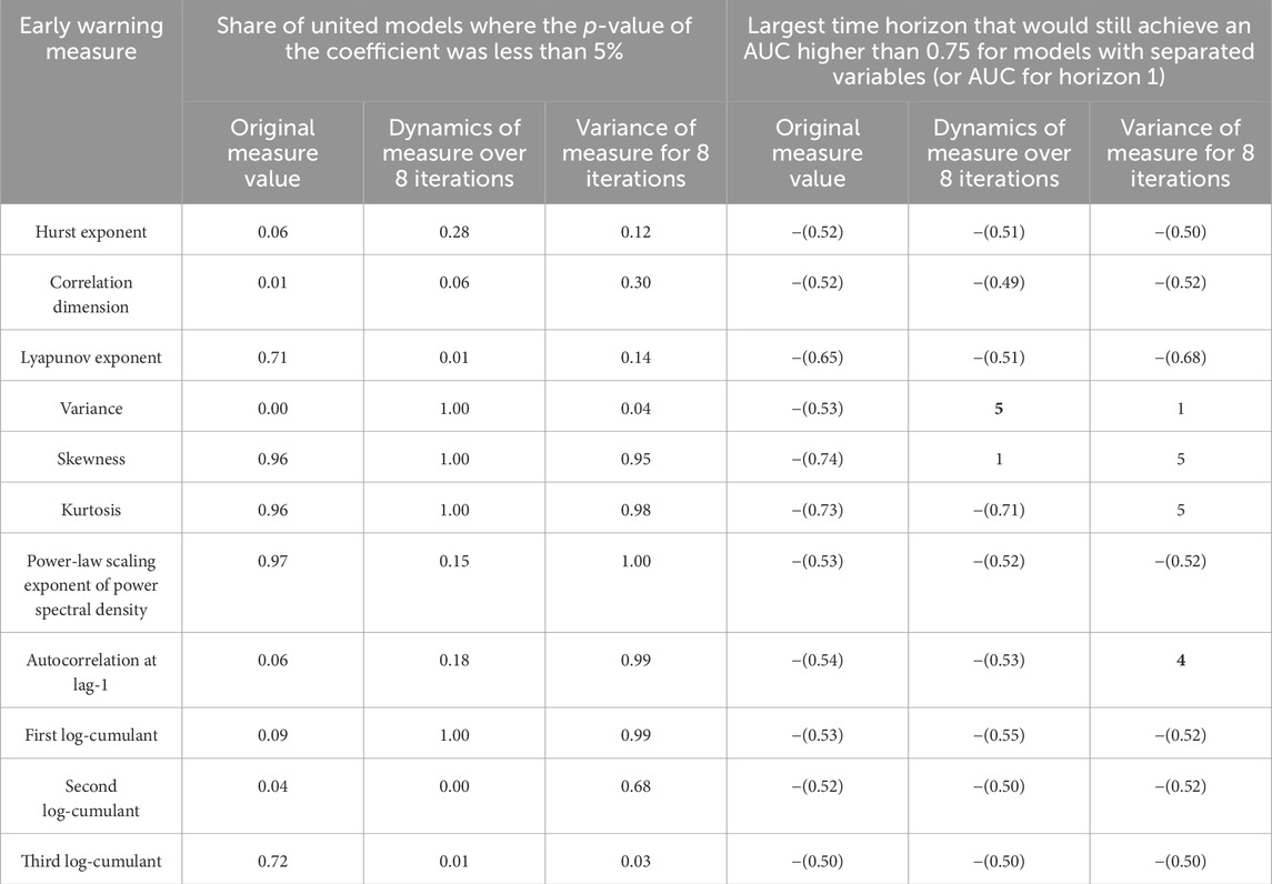
Table 1. Efficiency comparison for EWM and their modifications on the stock market data.

3.2 Phenomenological model of stock exchange self-organization into a critical state

As shown in Subsection 3.1, a stock exchange self-organizes into a critical state and stays in this state for a certain number of hours, determined by the share of a public company that is traded on the exchange. In other words, each segment of a stock exchange has a different time duration for it to be in a critical state. By a stock exchange segment we mean a set of trading platforms (world stock exchanges) and market traders involved in buying/selling a share of some public company. Hereinafter we use the term stock exchange and understand it as a segment of the stock exchange.

A stock exchange in a critical state is characterized by a near-1 autocorrelation for stock’s volume and a power law for the power spectral density of stock’s volume with degree exponent from 1 to 2. The dynamics of a system with such characteristics is known as the avalanche-like dynamics of the system observed when it is in a critical state, also known as the edge of a phase transition (e.g., see the paper [14]). One of the first and most studied models of self-organization of systems into a critical state is the SCA model, which explains the spontaneous emergence of a system into a critical state with its avalanche-like behavior. Therefore, we used SCA not only as a system generating test dynamical series (see Subsection 2.1), but also as a basic, systemically isomorphic model of SCA in the context of systems theory, the stock market model. In other words, when building a stock exchange model, we use the analogy of structure (Chung-Lu graph of SCA and complex network of exchange transaction network), the nature of elements (stable/unstable vertices of SCA and passive/active stock exchange traders) and links (collapse of unstable vertices of SCA and buy/sell transaction of a public company share) between the elements of SCA and stock exchange.

Let $\mathrm{\Gamma }$ be a planar graph of exchange transactions with nodes $\left(k,m\right)$, for which $k,m\mathbb{\in }\mathbb{Z}$ are the ultrametric coordinates of the exchange traders. As $\mathrm{\Gamma }$ we used Chung-Lu graphs with two-parameter degree distribution of edges as the most common and empirically validated model determining the topological structure of exchange transactions (e.g., see the papers [48–53]).

Let $h\left(k,m\right)\in {\mathbb{Z}}^{+}\cup \left\{0\right\}$ be the entropy as a measure of uncertainty of information about the share of some public company, which is available to the stock exchange trader $\left(k,m\right)$. Let $h\left(k,m\right)$ be denoted by $h_c$, which defines the threshold value of entropy for a trader $\left(k,m\right)$ to sell a share to its nearest neighbour, for example, $\left(k+1,m\right)$, in the graph $\mathrm{\Gamma }$.

Thus, each exchange trader with some number of shares can be in both an active state, denoted $\left(k_a,m_a\right)$, and a passive state, denoted $\left(k_p,m_p\right)$. Trader $\left(k_a,m_a\right)$ is in the active state if the corresponding entropy $h\left(k_p,m_p\right)$ is not less than a critical value, $h_c$. Otherwise, trader $\left(k,m\right)$ is in the passive state. Trader $\left(k_a,m_a\right)$, having uncertainty about a stock at least $h_c$, seeks to get rid of such stocks. As a result, trader $\left(k_a,m_a\right)$ sells the shares to his nearest neighbour in the graph $\mathrm{\Gamma }$, e.g., trader $\left(k_p,m_p\right)=\left(k_a+1,m_a\right)$, who is in the passive state and has uncertainty about the share less than $h_c$. In this case, trader $\left(k_p,m_p\right)$ has more information about the tendencies of the price behavior of the bought stock. After the local exchange transaction of buy/sell $\left(k_a,m_a\right)\to \left(k_p,m_p\right)$ the trader $\left(k_a,m_a\right)$ becomes passive until he receives some information which increases the uncertainty of information about tendencies of price behavior of the share. The source of such information can be a report of a public company, mass media news or some insider information. On the contrary, after the exchange transaction $\left(k_a,m_a\right)\to \left(k_p,m_p\right)$ trader $\left(k_p,m_p\right)$ enters an active state in which he is ready to sell the stock to some of his passive nearest neighbours. Figure 1A shows local exchange collapses.

Figure 1

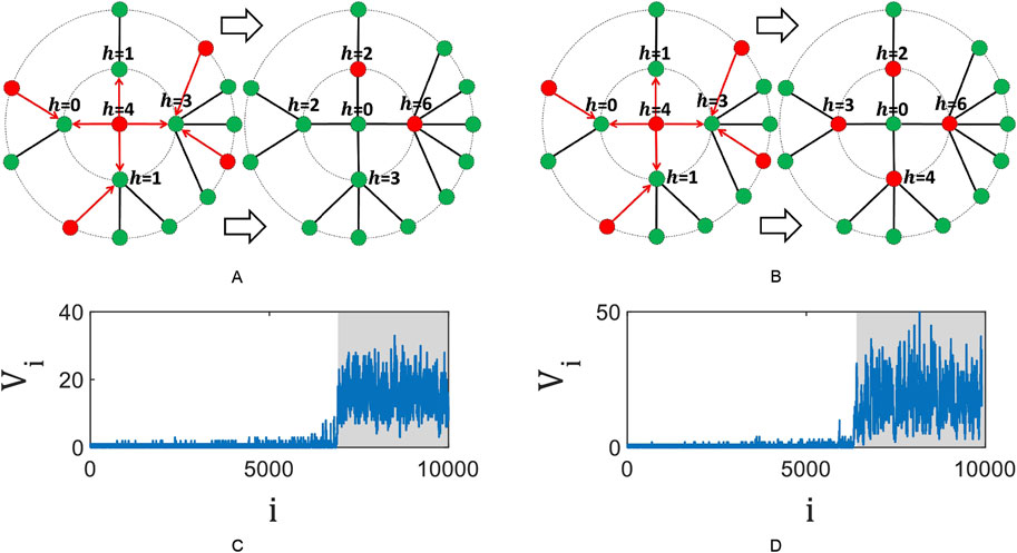
Figure 1. Local exchange transactions leading to self-organization of the stock exchange to the edge of the second-order phase transition (A) and to the edge of the first-order phase transition (B). The symbol $h$ denotes the entropy. Model series of exchange volume corresponding to self-organization of the stock exchange to the edge of the second-order phase transition (C) and to the edge of the first-order phase transition (D). The gray region indicates the edge of a phase transition.

Self-organization of the stock exchange into a critical state occurs as a result of its pumping (perturbation) and relaxation at each iterative step. Each iteration starts with pumping and ends with complete relaxation of the stock exchange. Information pumping of the stock exchange leads to an increase in entropy or to an increase in the volatility of the stock, i.e., to an increase in the possibility of the stock price to change in any direction. Relaxation of the stock exchange occurs as a result of local exchange transactions of buying/selling a share and is formally defined by the following rules:

$\begin{array}{c}h\left(k,m\right)\ge h_c\left(k,m\right)\\ \begin{array}{c}h\left(k,m\right)\to h\left(k,m\right)-h_c\left(k,m\right)\\ \begin{array}{c}h\left(\text{Ne}\left(k,m\right)\right)\to h\left(\text{Ne}\left(k,m\right)\right)+{\delta }_p\\ {\displaystyle \sum _{p=1}^{z_c\left(k,m\right)}}{\delta }_p=h_c\left(k,m\right),{\delta }_p\ge 0\end{array}\end{array}\end{array},(4)$

where $h_c\left(k,m\right)$ is the critical for trader $\left(k,m\right)$ entropy value equal to the number of its nearest neighbors in the graph $\mathrm{\Gamma }$; $\text{Ne}\left(k,m\right)$ is the nearest neighbour of trader $\left(k,m\right)$ in the graph $\mathrm{\Gamma }$; ${\delta }_m$ is a random number taking values from the set ${\mathbb{Z}}^{+}\cup \left\{0\right\}$.

The model based on the Equation 4 explains the phenomenon of self-organization of the stock exchange into a critical state starting from some critical iteration $i_c$. Starting from initial public offering ($i=0$) and up to the moment of completion of the subcritical phase ($0<{i<i}_c$), the stock exchange observes a small number of share buy/sell transactions, which quickly decay in ultrametric space and time. The global information pumping of the stock exchange to a critical entropy value $H_c$ brings the stock exchange into the critical state (${i\ge i}_c$). Staying in a small neighbourhood of $H_c$ the stock exchange is unstable to small information perturbations. In such an unstable state, a small entropy increment ($H_c\pm \delta H$) is sufficient for the stock exchange to experience avalanches of stock buy/sell transactions. The stock volume series, $V_i$, in the critical state of the stock exchange (${i\ge i}_c$) is characterised by $\rho \left(1\right)=1$, $S\left(f\right)=f^{-1}$, and $p\left(\xi \right)={\xi }^{-2}$. The dynamic series $V_i$, demonstrating the dynamics of such self-organization, is presented in Figure 1C.

The above described self-organization of the stock exchange corresponds to its self-organization to the edge of the second-order phase transition. To describe the self-organization of the stock exchange to the edge of the first-order phase transition, the following changes in the rules of model (1) are sufficient. Any stock exchange trader $\left(k,m\right)$, who is in the passive state $\left(k_p,m_p\right)$, can move to the active state $\left(k_a,m_a\right)$ if $h\left(k,m\right)\ge h_c\left(k,m\right)$, and if he has purchased a share from at least one of his nearest neighbours. The latter is characteristic of the stock exchange during the period of increased activity of its traders, i.e., when each trader $\left(k_p,m_p\right)$, having bought a share from a neighboring trader, passes to the state $\left(k_a,m_a\right)$ independently of the entropy value $h\left(k,m\right)$. Being in the state $\left(k_a,m_a\right)$ a trader immediately tries to sell the bought share. Such a stock exchange is dominated by speculative buy/sell transactions of the stock. Figure 1B demonstrates the corresponding local stock exchange collapses. The dynamic series $V_i$, demonstrating the dynamics of self-organization of the stock exchange to the edge of the first-order phase transition, is presented in Figure 1D. Local exchange transactions of buying/selling a stock are formally determined by the following rules:

$\begin{array}{l}h\left(k,m\right)\ge h_c\left(k,m\right)\vee 2\le h\left(k,m\right)<h_c\left(k,m\right)\\ h\left(k,m\right)\ge h_c\left(k,m\right):\left\{\begin{array}{l}h\left(k,m\right)\to h\left(k,m\right)-h_c\left(k,m\right)\\ \begin{array}{l}h\left(\text{Ne}\left(k,m\right)\right)\to h\left(\text{Ne}\left(k,m\right)\right)+{\delta }_p\\ {\displaystyle \sum _{p=1}^{z_c\left(k,m\right)}}{\delta }_p=h_c\left(k,m\right),{\delta }_p\ge 0\end{array}\end{array}\right.\\ 2\le h\left(k,m\right)<h_c\left(k,m\right):\left\{\begin{array}{l}h\left(k,m\right)\to h\left(k,m\right)-h_c\left(k,m\right)\\ h\left(\text{Ne}\left(k,m\right)\right)\to h\left(\text{Ne}\left(k,m\right)\right)+{\delta }_p\\ \begin{array}{l}{\displaystyle \sum _{p=1}^{z_c\left(k,m\right)}}{\delta }_p=h_c\left(k,m\right),{\delta }_p\ge 0\\ h\left(\text{Ne}\left(k,m\right)\right)\to h\left(\text{Ne}\left(k,m\right)\right)+1\end{array}\end{array}\right.\end{array}.(5)$

Note that the proposed models which are based on the Equation 5 determine the self-organization of the stock exchange into a critical state, which does not require fine-tuning of the control parameter $H$ to the critical value $H_c$. Exit to the critical state is achieved as a result of perturbation and relaxation of the stock exchange, as well as the above-described nonlinear interactions between the stock exchange traders.

3.3 Early warning signals for stock exchange self-organization into a critical state

One of the results of our calculations is the independence of the behavior of the series for any of the EWMs in the vicinity of the critical onset from the specific public company for which the EWM series was calculated. The EWMs series differ only in their noise and early warning time (see Subsection 3.1). Apparently, the self-organization of a stock exchange into a critical state is a universal phenomenon. Therefore, we will limit ourselves to discussing the behavior of a series of EWMs for stock exchange transactions of, for example, Ameris Bancorp. This company is a bank holding company that, through its subsidiary Ameris Bank, provides banking services to its retail and commercial customers.

Figure 2 shows the behavior of the moving average smoothed series of EWMs that are obtained for the stock volume series of Ameris Bancorp from 10:30 7 February 2022 to 15:30 p.m. 5 February 2024. The smoothing of these series reduced the number of false early warning signals.

Figure 2

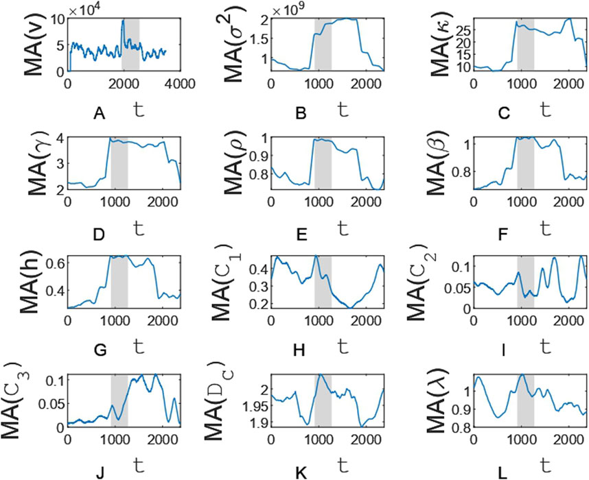
Figure 2. Moving average series for the stock volume series (A), variance (B), kurtosis (C), skewness (D), autocorrelation at lag-1 (E), power-law scaling exponent of the power spectral density (F), generalized Hurst exponent (G), position of the multifractal spectrum maximum (H), multifractal spectrum width (I), multifractal spectrum skewness (J), correlation dimension (K), and largest Lyapunov exponent (L). The gray region indicates the edge of a phase transition.

The MA100 series obtained for the stock volume series increases sharply in the vicinity of the critical point, $t_c$, i.e., the time when the stock exchange starts to self-organize into a critical state (see Figure 2A). The time $t_c$ corresponds to 15:30 10 March 2023. The MA100 series increased by 20% compared to the volumes of the previous 5 hours at 11:30 10 March 2023. Therefore, no more than 4 h are given to take preventive measures to avoid self-organization of the stock exchange into a critical state.

The above described behavior of the MA100 series is a consequence of the critical slowdown of the stock exchange, the manifestation of which is an increase in the average amplitude of stochastic fluctuations of the order parameter (stock volume). Indeed, in the vicinity of $t_c$ there is an increase in the average amplitude of stochastic fluctuations of stock volume, which leads to an increase in MA100.

Other evidence of the critical slowing down of the stock market in the vicinity of $t_c$ is the behavior of window variance (see Figure 2B), kurtosis (see Figure 2C), skewness (see Figure 2D), autocorrelation at lag-1 (see Figure 2E), and power-law scaling exponent of the power spectral density (see Figure 2F) characteristic of the critical slowing down. These measures increase sharply in the neighborhood of $t_c$. At the same time, kurtosis and skewness take positive values, which is a consequence of the increase in the amplitude of stochastic fluctuations of stock volume. Moreover, autocorrelation at lag-1 and power-law scaling exponent of the power spectral density take values close to 1 in the time interval from 15:30 10 March 2023 to 15:30 p.m. 27 March 2023. Thus, the stock exchange has been in a critical state for 17 trading days. In Figure 2, the interval corresponding to the critical state, or the edge of the phase transition, is shown as a gray region. The stock exchange in this interval is characterized by abnormal fluctuations of the stock volume and strong, close to 1, correlation between neighboring elements of the sequence of values of the stock volume.

Another sign of the stock volume series approaching $t_c$ is a sharp increase of the generalised Hurst exponent to the value of 0.63 in the interval corresponding to the critical state (see Figure 2G). Consequently, if the stock volume series is considered as a real-time series, the sequence of values of the stock volume becomes more correlated as the stock volume series approaches $t_c$. The stock volume series corresponding to the critical state is a time series with long-term positive autocorrelation. Based on the fact that the position of the center of the multifractal spectrum, $h_0=C_1$, shifts to the right as the stock approaches $t_c$ (see Figure 2H), the stock volume series becomes more singular in the vicinity of $t_c$. The width, $W=C_2$, and skewness, $S=C_3$, of the multifractal spectrum increase as the stock volume series approaches $t_c$ (see Figures 2I, J). The multifractal spectrum becomes symmetric, $C_3=S=1$, at $t=t_c$ (see Figure 2J). Since $S<1$ at $t<t_c$,the multifractal spectrum for the subcritical phase, $t<t_c$, is asymmetric with small fluctuations dominating the stock volume. Consequently, in the neighborhood of $t_c$ the stock volume series becomes a more inhomogeneous series with dominance of large fluctuations. Thus, the described behavior of multifractal measures and Hurst exponent are early warning signals for the stock exchange self-organization into a critical state.

Let us consider the behavior of the series of EWMs, the calculation of which is based on the reconstruction of the phase space of the stock exchange. As the stock exchange approaches $t_c$ the correlation dimension of the reconstructed attractor increases (see Figure 2K), hence the fractal structure of the attractor becomes more complex and the chaotic behavior of the stock exchange becomes more complicated. The most complex chaotic behavior of the stock exchange, corresponding to the highest value of the correlation dimension, is observed in its critical state. An indication of the increasing complexity of the chaotic behavior of the stock exchange is also an increase in the largest Lyapunov exponent, which is positive, as the stock volume series approaches $t_c$ (see Figure 2L). The most complex chaotic dynamics of the stock exchange also corresponds to its critical state, since the largest value of the exponent is observed in the time interval corresponding to the critical state.

4 Conclusion

The stock exchange self-organizes to the edge of a phase transition. The duration of a stock exchange at the edge ranges from 7 to 19 trading hours and depends on the public company whose shares are traded on the stock exchange. We set such durations for public company stocks from the Russel 3,000 index, which measures the performance of the 3,000 largest US companies by market capitalization. Perhaps the result of finding time intervals corresponding to the edge of a phase transition for more public company stocks would be a longer range of trading day durations. In addition, further research of the time intervals should be focused on the analysis of the stock volume series with higher frequency, such as every second and every minute series, but adjusted for the volumes of pre-planned execution of deals. Analyzing such series will allow you to identify the time intervals that cannot be identified in hourly stock volume. For example, high-frequency trading implies the conclusion of a large number of buy/sell transactions in a fraction of a second and it may take several seconds for the stock exchange to self-organize to the edge of a phase transition. If the duration of the stock exchange on the edge of a phase transition is less than 1 h, the analysis of the hourly stock volume series will not allow to identify the time interval corresponding to the edge. The best identification will be obtained when analyzing the second-by-second series for the stock volume. In addition, the transition to more frequent stock volume series will allow to obtain segments of series corresponding to the edge, of longer length and possibly of sufficient length to obtain a reliable estimate for the power-law scaling exponent of the power spectral density. Comparison of such estimates will allow us to determine which of the critical states, i.e., the edge of the phase transition of the first or second kind, corresponds to the detected time interval.

The sandpile cellular automaton model of self-organization to the edge of a phase transition is based on the idea that information drives stock markets (e.g., see the paper [54]). Self-organization of a stock exchange occurs in a discrete number of steps, each of which begins with an information perturbation of the stock exchange and ends with its relaxation. If the information pumping results in supra-critical uncertainty, or entropy, in the price behavior of a stock for some traders, then the stock exchange relaxation occurs as a result of these traders’ execution of stock buy/sell transactions, which reduces the uncertainty in the price behavior of the stock for the traders. We have considered implementations of the model under the assumption that all traders are characterized by a single critical level of uncertainty. In the context of effective market hypothesis such assumption is quite reasonable, but it is not applicable when analyzing the stock market in the context of fractal market hypothesis. Therefore, further improvement of the model should be focused on the study of the influence of the type and parameters of the probability distribution of critical uncertainty on the behaviour of the stock volume series when the stock exchange approaches the edge of a phase transition, as well as on the edge. Another direction of the model improvement is the introduction of an assumption about the existence of some critical uncertainty of price behaviour, which determines the condition of buying a share of a public company. Moreover, the critical uncertainty when buying a share is not equal to the critical uncertainty when selling it.

The studied early warning measures, first of all MA100, variance, kurtosis and skewness as the most effective ones, can be used to detect early warning signals for self-organization of the stock exchange to the edge of a phase transition in real-time early warning systems. Such signals are important for the regulator of trading on the stock exchange, as they allow detecting illegal exchange operations. The volume indicator reflects an increase or decrease in the activity of traders on the stock exchange. Therefore, early detection of the time interval in the stock volume series corresponding to the stock exchange’s edge will allow a trader to make reasonable and timely changes in his trading strategy. As a rule, traders correlate the volume indicator with the direction of the stock price movement. If the stock price is rising along with the volume, the price growth is likely to continue. High volume (25% higher than average) when the stock price reaches a new high is a harbinger of a strong increase in the stock price. Traders should refrain from selling existing shares and/or buy shares while they are cheap and sell them when they rise in price. If the share price is declining while volume is rising, the stock market is dominated by stock sellers - the trader should refrain from speculating in the stock.

Data availability statement

The datasets presented in this study can be found in online repositories. The names of the repository/repositories and accession number(s) can be found below: https://github.com/lebedevaale/early_warning_model.

Author contributions

AD: Conceptualization, Formal Analysis, Funding acquisition, Methodology, Validation, Writing–original draft. AL: Data curation, Investigation, Resources, Software, Validation, Visualization, Writing–review and editing. VK: Data curation, Funding acquisition, Project administration, Supervision, Writing–review and editing. VD: Conceptualization, Data curation, Funding acquisition, Investigation, Project administration, Visualization, Writing–review and editing.

Funding

The author(s) declare that financial support was received for the research, authorship, and/or publication of this article. The work is an output of a research project implemented as part of the Basic Research Program at the National Research University Higher School of Economics (HSE University).

Conflict of interest

The authors declare that the research was conducted in the absence of any commercial or financial relationships that could be construed as a potential conflict of interest.

Generative AI statement

The author(s) declare that no Generative AI was used in the creation of this manuscript.

Publisher’s note

All claims expressed in this article are solely those of the authors and do not necessarily represent those of their affiliated organizations, or those of the publisher, the editors and the reviewers. Any product that may be evaluated in this article, or claim that may be made by its manufacturer, is not guaranteed or endorsed by the publisher.

References

1. Bak P, Tang C, Wiesenfeld K. Self-organized criticality: an explanation of the 1/f noise. Phys Rev Lett (1987) 59:381–4. doi:10.1103/PhysRevLett.59.381

PubMed Abstract | CrossRef Full Text | Google Scholar

2. Watkins NW, Pruessner G, Chapman SC, Crosby NB, Jensen HJ. 25 Years of self-organized criticality: concepts and controversies. Space Sci Rev (2016) 198:3–44. doi:10.1007/s11214-015-0155-x

CrossRef Full Text | Google Scholar

3. Walter N, Hinterberger T. Self-organized criticality as a framework for consciousness: a review study. Front Psychol (2022) 13:911620. doi:10.3389/fpsyg.2022.911620

PubMed Abstract | CrossRef Full Text | Google Scholar

4. Plenz D, Ribeiro TL, Miller SR, Kells PA, Vakili A, Capek EL. Self-organized criticality in the brain. Front Phys (2021) 9:639389. doi:10.3389/fphy.2021.639389

CrossRef Full Text | Google Scholar

5. Zhukov D. How the theory of self-organized criticality explains punctuated equilibrium in social systems. Methodological Innov (2022) 15:163–77. doi:10.1177/20597991221100427

CrossRef Full Text | Google Scholar

6. Tadiс B, Melnik R. Self-organized critical dynamics as a key to fundamental features of complexity in physical, biological, and social networks. Dynamics (2021) 1:181–97. doi:10.3390/dynamics1020011

CrossRef Full Text | Google Scholar

7. Zhukov D. Personality and society in the theory of self-organized criticality. Changing Societies and Personalities (2023) 7:10–33. doi:10.15826/csp.2023.7.2.229

CrossRef Full Text | Google Scholar

8. Smyth WD, Nash JD, Moum JN. Self-organized criticality in geophysical turbulence. Scientific Rep (2019) 9:3747. doi:10.1038/s41598-019-39869-w

PubMed Abstract | CrossRef Full Text | Google Scholar

9. Mikaberidze G, Plaud A, D'Souza RM. Dragon kings in self-organized criticality systems. Phys Rev Res (2023) 5:L042013. doi:10.1103/PhysRevResearch.5.L042013

CrossRef Full Text | Google Scholar

10. Alodjants AP, Bazhenov AY, Khrennikov AY, Bukhanovsky AV. Mean-field theory of social laser. Scientific Rep (2022) 12:8566. doi:10.1038/s41598-022-12327-w

PubMed Abstract | CrossRef Full Text | Google Scholar

11. Alodjants AP, Tsarev DV, Avdyushina AE, Khrennikov AY, Boukhanovsky AV. Quantum-inspired modeling of distributed intelligence systems with artificial intelligent agents self-organization. Scientific Rep (2024) 14:15438. doi:10.1038/s41598-024-65684-z

PubMed Abstract | CrossRef Full Text | Google Scholar

12. Jarai AA. The sandpile cellular automaton. Complexity Comput (2018) 27:79–88. doi:10.1007/978-3-319-65558-1_6

CrossRef Full Text | Google Scholar

13. Shapoval A, Shnirman M. Explanation of flicker noise with the Bak-Tang-Wiesenfeld model of self-organized criticality. Phys Rev E (2024) 110:014106. doi:10.1103/PhysRevE.110.014106

PubMed Abstract | CrossRef Full Text | Google Scholar

14. Buendia V, di Santo S, Bonachela JA, Muñoz MA. Feedback mechanisms for self-organization to the edge of a phase transition. Front Phys (2020) 8:333. doi:10.3389/fphy.2020.00333

CrossRef Full Text | Google Scholar

15. Song S, Li H. Early warning signals for stock market crashes: empirical and analytical insights utilizing nonlinear methods. EPJ Data Sci (2024) 13:16. doi:10.1140/epjds/s13688-024-00457-2

CrossRef Full Text | Google Scholar

16. Ran M, Tang Z, Chen Y, Wang Z. Early warning of systemic risk in stock market based on EEMD-LSTM. PLoS One (2024) 19:e0300741. doi:10.1371/journal.pone.0300741

PubMed Abstract | CrossRef Full Text | Google Scholar

17. Bartolozzi M, Leinweber D, Thomas A. Self-organized criticality and stock market dynamics: an empirical study. Physica A: Stat Mech its Appl (2005) 350:451–65. doi:10.1016/j.physa.2004.11.061

CrossRef Full Text | Google Scholar

18. Stanley HE, Amaral LAN, Buldyrev SV, Gopikrishnan P, Plerou V, Salinger MA. Self-organized complexity in economics and finance. PNAS (2002) 99:2561–5. doi:10.1073/pnas.022582899

PubMed Abstract | CrossRef Full Text | Google Scholar

19. Goncalves CP. Chaos-induced self-organized criticality in stock market volatility-an application of smart topological data analysis. Int J Swarm Intelligence Evol Comput (2023) 12:331. doi:10.35248/2090-4908.22.12.331

CrossRef Full Text | Google Scholar

20. Chandra A, Reinstein A. A study of production, stock prices and self-organized criticality. Rev Account Finance (2004) 3:20–39. doi:10.1108/eb043406

CrossRef Full Text | Google Scholar

21. Kaki B, Farhang N, Safari H. Evidence of self-organized criticality in time series by the horizontal visibility graph approach. Scientific Rep (2022) 12:16835. doi:10.1038/s41598-022-20473-4

PubMed Abstract | CrossRef Full Text | Google Scholar

22. Diks C, Hommes C, Wang J. Critical slowing down as an early warning signal for financial crises? Empirical Econ (2019) 57:1201–28. doi:10.1007/s00181-018-1527-3

CrossRef Full Text | Google Scholar

23. Kang BS, Park C, Ryu D, Song W. Phase transition phenomenon: a compound measure analysis. Physica A: Stat Mech its Appl (2015) 428:383–95. doi:10.1016/j.physa.2015.02.044

CrossRef Full Text | Google Scholar

24. Biondo AE, Pluchino A, Rapisarda A. Order book, financial markets, and self-organized criticality. Chaos, Solitons and Fractals (2016) 88:196–208. doi:10.1016/j.chaos.2016.03.001

CrossRef Full Text | Google Scholar

25. Schmidhuber C. Financial markets and the phase transition between water and steam. Physica A (2022) 592:126873. doi:10.1016/j.physa.2022.126873

CrossRef Full Text | Google Scholar

26. Dmitriev A, Lebedev A, Kornilov V, Dmitriev V. Multifractal early warning signals about sudden changes in the stock exchange states. Complexity (2022) 2022:8177307. doi:10.1155/2022/8177307

CrossRef Full Text | Google Scholar

27. Biondo AE, Pluchino A, Rapisarda A. Modeling financial markets by self-organized criticality. Phys Rev E (2015) 92:042814. doi:10.1103/PhysRevE.92.042814

PubMed Abstract | CrossRef Full Text | Google Scholar

28. Rao B, Yi D, Zhao C. Self-organized criticality of individual companies: an empirical study. Third Int Conf Nat Comput (ICNC 2007) (2007) 481–7. doi:10.1109/ICNC.2007.654

CrossRef Full Text | Google Scholar

29. Zhang D, Zhuang Y, Tang P, Peng H, Han Q. Financial price dynamics and phase transitions in the stock markets. The Eur Phys J B (2023) 96:35. doi:10.1140/epjb/s10051-023-00501-6

PubMed Abstract | CrossRef Full Text | Google Scholar

30. Chung F, Lu L. Connected components in random graphs with given expected degree sequences. Ann Combinatorics (2002) 6:125–45. doi:10.1007/pl00012580

CrossRef Full Text | Google Scholar

31. Manna SS. Sandpile models of self-organized criticality. Curr Sci (1999) 77:388–93. Available from: https://www.jstor.org/stable/24102958. (Accessed December 24, 2024).

Google Scholar

32. di Santo S, Burioni R, Vezzani A, Muñoz MA. Self-organized bistability associated with first-order phase transitions. Phys Rev Lett (2016) 116:240601. doi:10.1103/PhysRevLett.116.240601

PubMed Abstract | CrossRef Full Text | Google Scholar

33. George SV, Kachhara S, Ambika G. Early warning signals for critical transitions in complex systems. Physica Scripta (2023) 98:072002. doi:10.1088/1402-4896/acde20

CrossRef Full Text | Google Scholar

34. Zhao L, Li W, Yang C, Han J, Su Z, Zou Y. Multifractality and network analysis of phase transition. PLoS ONE (2017) 12:e0170467. doi:10.1371/journal.pone.0170467

PubMed Abstract | CrossRef Full Text | Google Scholar

35. Hasselman F. Early warning signals in phase space: geometric resilience loss indicators from multiplex cumulative recurrence networks. Front Physiol (2022) 13:859127. doi:10.3389/fphys.2022.859127

PubMed Abstract | CrossRef Full Text | Google Scholar

36. Dmitriev A, Lebedev A, Kornilov V, Dmitriev V. Twitter self-organization to the edge of a phase transition: discrete-time model and effective early warning signals in phase space. Complexity (2023) 2023:1–13. doi:10.1155/2023/3315750

CrossRef Full Text | Google Scholar

37. Astfalck LC, Sykulski AM, Cripps EJ. Debiasing Welch’s method for spectral density estimation. Biometrika (2024) 111:1313–29. doi:10.1093/biomet/asae033

CrossRef Full Text | Google Scholar

38. Shanshan Z, Jiang Y, He W, Mei Y, Xie X, Wan S. Detrended fluctuation analysis based on best-fit polynomial. Front Environ Sci (2022) 10. doi:10.3389/fenvs.2022.1054689

CrossRef Full Text | Google Scholar

39. Achour R, Li Z, Selmi B, Wang T. A multifractal formalism for new general fractal measures. Chaos, Solitons and Fractals (2024) 181:114655. doi:10.1016/j.chaos.2024.114655

CrossRef Full Text | Google Scholar

40. Nazarimehr F, Jafari S, Hashemi Golpayegani SMR, Sprott JC. Can Lyapunov exponent predict critical transitions in biological systems? Nonlinear Dyn (2017) 88:1493–500. doi:10.1007/s11071-016-3325-9

CrossRef Full Text | Google Scholar

41. Takens F. Detecting strange attractors in turbulence. Dynamical systems and turbulence, warwick 1980. Lecture Notes Mathematics (1981) 898:366–81. doi:10.1007/BFb0091924

CrossRef Full Text | Google Scholar

42. Weber I, Oehrn CR. NoLiTiA: an open-source toolbox for non-linear time series analysis. Front Neuroinformatics (2022) 16:876012. doi:10.3389/fninf.2022.876012

PubMed Abstract | CrossRef Full Text | Google Scholar

43. Rosenstein MT, Collins JJ, De Luca CJ. A practical method for calculating largest Lyapunov exponents from small data sets. Physica D: Nonlinear Phenomena (1993) 65:117–34. doi:10.1016/0167-2789(93)90009-P

CrossRef Full Text | Google Scholar

44. Dmitriev A, Lebedev A, Kornilov V, Dmitriev V. Effective precursors for self-organization of complex systems into a critical state based on dynamic series data. Front Phys (2023) 11. doi:10.3389/fphy.2023.1274685

CrossRef Full Text | Google Scholar

45. Mooney CZ, Duval RD. Bootstrapping: a nonparametric approach to statistical inference. Newbury Park, CA, USA: Sage Publications (1993).

Google Scholar

46. Chib S. Analysis of multivariate probit models. Biometrika (1998) 85:347–61. doi:10.1093/biomet/85.2.347

CrossRef Full Text | Google Scholar

47. Berger VW, Zhou Y. Kolmogorov-Smirnov test: overview. Wiley StatsRef: Statistics Reference Online (2024). doi:10.1002/9781118445112.stat06558

CrossRef Full Text | Google Scholar

48. Tao B, Dai HN, Wu J, Ho IWH, Zheng Z, Cheang CF. Complex network analysis of the bitcoin transaction network. IEEE Trans Circuits Syst Express Briefs (2022) 69:1009–13. doi:10.1109/TCSII.2021.3127952

CrossRef Full Text | Google Scholar

49. Jihun P, Cho CH, Lee JW. A perspective on complex networks in the stock market. Front Phys (2022) 10. doi:10.3389/fphy.2022.1097489

CrossRef Full Text | Google Scholar

50. Huang W, Wang H, Wei Y, Chevallier J. Complex network analysis of global stock market co-movement during the COVID-19 pandemic based on intraday open-high-low-close data. Financial Innovation (2024) 10:7. doi:10.1186/s40854-023-00548-5

CrossRef Full Text | Google Scholar

51. Moghadam HE, et al. Complex networks analysis in Iran stock market: the application of centrality. Physica A (2019) 531:121800. doi:10.1016/j.physa.2019.121800

CrossRef Full Text | Google Scholar

52. Wang Z, Zhang G, Ma X, Wang R. Study on the stability of complex networks in the stock markets of key industries in China. Entropy (2024) 26:569. doi:10.3390/e26070569

PubMed Abstract | CrossRef Full Text | Google Scholar

53. Liu XF, Tse CK. A complex network perspective of world stock markets: synchronization and volatility. Int J Bifurcation Chaos (2012) 22:1250142. doi:10.1142/S0218127412501428

CrossRef Full Text | Google Scholar

54. Szczygielski JJ, Charteris A, Bwanya PR, Brzeszczyński J. Google search trends and stock markets: sentiment, attention or uncertainty? Int Rev Financial Anal (2024) 91:102549. doi:10.1016/j.irfa.2023.102549

CrossRef Full Text | Google Scholar