Shallow crustal structure detection of the upper crust at Anqiu-Juxian Fault in the Tanlu fault zone

Within the Tan-Lu Fault Zone, the largest active tectonic belt in eastern China, the Anqiu-Juxian Fault exhibits the most recent activity period, evident surface traces, and highest seismic hazard, making it a Holocene active fault. This study utilized the vertical component continuous data observed by 100 short-period temporary stations from August 1–21, 2023, and extracted 1,944 Rayleigh wave group velocity dispersion curves within the period of 0.2–4 s. Using the direct surface wave tomography method, we calculated a high-resolution 3-D shear-wave velocity structure at depths of 0.2–1.25 km within the study area. Our results are summarized as follows: 1) The development of faults F₁, F₂, and F₅ in the Tan-Lu Fault Zone highly correlated with the shear-wave velocity anomalies at depths >0.8 km. Specifically, fault F₅ comprised two boundary faults, F_5-1 and F_5-2, which together controlled a Cenozoic depression covered by a thick, low-velocity sediment layer. 2) The complex velocity structure characteristics in the Suqian area revealed that the influence of faults on the sedimentary layers in the Suqian area was not expressed as an overall uplift or subsidence of the block but rather as differential subsidence. 3) Near Sankeshu, the F₅ fault formed a small pull-apart basin. The latest activity in this pull-apart basin has shifted to the fault in the center of the basin, indicating that the pull-apart basin has entered the extinction stage.

1 Introduction

The Tan-Lu Fault Zone is the largest active fault zone in eastern China, extending from Luobei in Heilongjiang Province in the north to Guangji in Hubei Province in the south, spanning a length of up to 2,400 km, being an important tectonic boundary. It traverses the eastern part of mainland China, influencing crustal development, tectonic evolution, and seismic activity [1, 2]. Numerous destructive earthquakes have been recorded along the Tan-Lu Fault Zone, such as the Tancheng M8.5 earthquake on 25 July 1668, the Bohai Sea M7.5 earthquake on 13 June 1888, and the Haicheng M7.3 earthquake on 24 February 1975. Based on the tectonic activity characteristics, the Tan-Lu Fault Zone can be divided into four segments from north to south (Figure 1A) 1) the Hegang-Tieling segment, 2) the XiaLiaohe-LaizhouWan segment, 3) the Weifang-Jiashan segment, and 4) the Jiashan-Guangji segment. Among these segments, the Weifang-Jiashan segment is recognized as the most tectonically active [4, 5] and consists of the following five major faults, from east to west: the Shanzuokou-Sihong Fault (F₁), the Anqiu-Juxian Fault (F₅), the Xinyi-Xindian Fault (F₂), the Mohe-Lingcheng Fault (F₃), and–the Wangji Fault (F₄). Among these faults, fault F₅ is the most recently active Holocene fault among the Weifang-Jiashan segment of the Tan-Lu Fault Zone, exhibiting the most evident surface traces and the highest seismic hazard (Figure 1B) [3, 6].

Figure 1

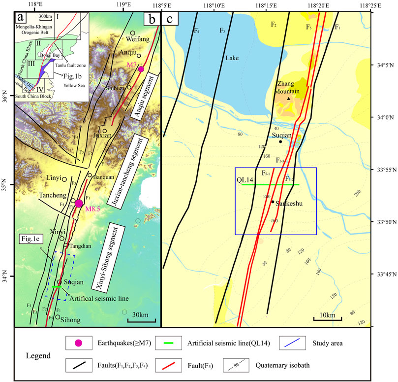
Figure 1. (A) Topographic map. (B) Fault distribution map of the Weifang–Jiashan segment of the Tanlu fault zone. F₁: Shanzuokou-Sihong Fault; F₂: Xinyi-Xindian Fault; F₃: Mohe-Lingcheng Fault; F₄: Jiji-Wangji Fault; F₅: Anqiu-Juxian Fault. (C) Tectonic distribution of the Suqian segment of Anqiu-Juxian Fault. The blue box indicates our study area. (Adapted from Zhang et al. (2023)) [3].

The Anqiu M7 earthquake in 70 BCE (before common era) and the Tancheng M8.5 earthquake in 1668 were both associated with fault F₅ [4, 7]. The Jiangsu segment of fault F₅ is located between fault F₁ and fault F₂. Based on the spatial distribution and activity period, fault F₅ consists of three segments in a north-south direction: the Anqiu, Juxian-Tancheng, and Xinyi-Sihong segments (Figure 1B) [8, 9]. The late Quaternary activity characteristics of fault F₅ indicate that a major paleoseismic event has occurred since the Holocene [10, 11]. Several fault profiles were found from Nanmaling Mountain to Chonggang Mountain, these profiles suggest significant Holocene activity along the Jiangsu segment of fault F₅, with the most recent activity primarily characterized by thrusting movement, with a maximum displacement of 1 m. Overall, the Quaternary activity of fault F₅ was characterized by dextral strike-slip combined with thrusting movement, whereas localized regions were characterized by strike-slip with normal faulting. Since the late Pleistocene, fault F₅ has experienced multiple activities, showed significant activity during the Holocene, with seismic activity characterized by high intensity and low frequency [12].

Owing to its complex crustal structure and intense tectonic activity, numerous studies have been conducted on fault F₅ by previous researchers. For instance, Xu et al. (2016) performed a shallow seismic exploration of fault F₅ to determine its precise localization and development characteristics [13]. However, their study was limited to providing evidence of the existence, exact position, and recent activities of fault F₅ in Suqian area without further investigation. Cao et al. (2015) have reported major findings in the precise fault localization and activity research of the Suqian segment of fault F₅ through shallow seismic exploration and drilling combined profiling [14]. However, the limited coverage of shallow seismic profiles limits our understanding of continuity and variations in large horizontal strata. Meng et al. (2019) utilized ambient noise tomography to obtain a 3-D S-wave (shear-wave) velocity model for the central-southern section of the Tan-Lu Fault Zone [15]. Although the imaging results included our study area, the resolution of the shallow structures was low. Qin et al. (2020) obtained the shallow primary-wave velocity structure of the Tan-Lu Fault Zone using a first-break wave imaging method [16]; however, their study depth was primarily within 0.8 km, and there is a lack of research in deeper regions. Therefore, high-resolution 3-D S-wave velocity structures for the shallow part of the Suqian segment of fault F₅ remain warranted. Consequently, ambient noise tomography was used to investigate the shallow crustal structure of the Suqian segment of fault F₅ (Figure 1C).

This ambient noise tomography was first implemented in California, United States, in 2005 [17] and has since been widely accepted and extensively applied by seismologists. Using dispersion data within medium- or long-period ranges can invert the upper mantle and crustal velocity structure to investigate geodynamic processes underlying plate motion, earthquake nucleation, and magma transfer [18–21]. Utilizing dispersion data within short-period ranges can be inverted for high-resolution shear-wave velocity structures near the surface or in shallow parts of the crust, detection of hidden faults, geological disaster assessment, and 3D geological modeling [22–26].

This study used ambient noise data from a short-period dense array deployed in the Suqian segment of fault F₅. Our study area ranges from 118.2°E to 118.325°E and 33.815°N to 33.92°N (Figure 1C). We inverted the shallow S-wave velocity structure of the area by applying direct surface wave tomography [19]. By combining the velocity model with the regional tectonic background, we clarified the shallow crustal structure of the Suqian segment of fault F₅ and its influence on the sedimentary layers of the Suqian area. Our study findings will facilitate future studies on the extension characteristics of the Suqian segment of fault F₅ and aid in assessing seismic hazards.

2 Methods

In this study, we deployed 100 SmartSolo digital seismic stations with a main frequency of 5 Hz across fault F₅. The sampling rate was set at 1000 Hz (dt = 1 ms). Data recording was commenced on 1 August 2023 and concluded on 21 August 2023 covering a total duration of 20 days. The average station spacing was approximately 0.7 km. The station distribution is shown in Figure 2.

Figure 2

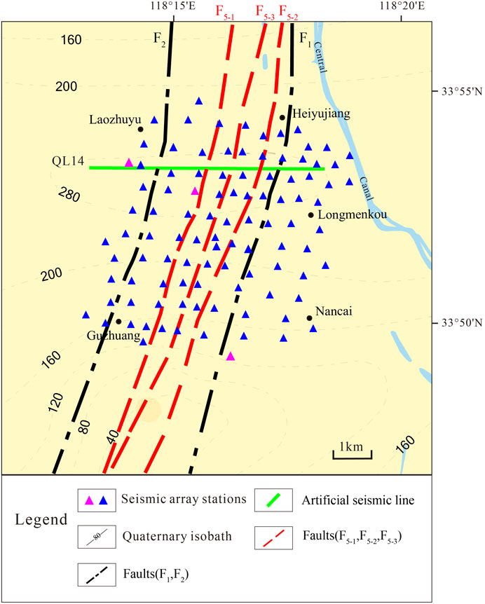
Figure 2. Station distribution in the Suqian area. The blue triangles represent the stations, the pink triangles represent stations G002, G008 and G048; the green line represents the artificial seismic line QL14 (Figure 11).

To increase the signal-to-noise ratio (SNR) and reduce computational time, the raw data from each station were decimated to 10 samples per period. Subsequently, the mean value and trend of the data were removed, then bandpass filtered in the period band 0.2–4 s. Besides, we performed the spectral whitening and temporal normalization before the calculation of cross-correlation in order to avoid the effects of earthquakes [27, 28]. Finally, cross-correlation was conducted to obtain the time-domain cross-correlation functions (CFs) between the two stations for each daily data. Figure 3A illustrates the CFs with SNR >4.5 in the period band of 0.2–4 s, revealing prominent Rayleigh surface-wave signals of 1.4 km/s. Figure 3B shows the normalized amplitudes of the CFs for all station pairs. It can be observed that most values of relative amplitude ratios are between 0.5 and 1, which means the differences in amplitude between positive- and negative-time CFs are insignificant. This indicates there will hardly be any significant bias in surface-wave dispersion measurements [29].

Figure 3

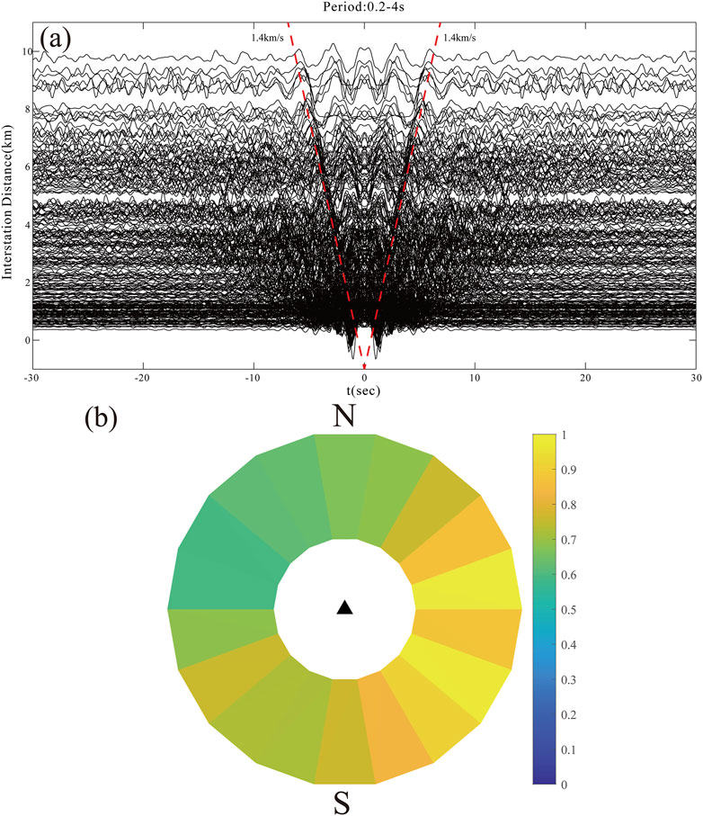
Figure 3. (A) Cross-correlation functions (CFs) with signal-to-noise ratio (SNR) > 4.5 in the 0.2–4 s period band obtained using the normalized linear stacking method. (B) Azimuthal dependence of the normalized amplitudes of CFs for all station pairs in the 0.2–4 s period band.

We employed a quick tracing method and an image analysis technique to extract the Rayleigh wave group velocity dispersion curves from the Empirical Green’s functions (EGFs) of all station pairs [18]. Two quality control criteria were followed during selection of the dispersion curves to get reasonable dispersion curves, which will be used to invert the S-wave model. Firstly, considering the far-field approximation, we excluded records where the interstation distance was less than twice the wavelength [22]. Secondly, for the inversion results to closely approximate the real conditions, only the dispersion curves with SNR >4.5 was used in this study.

Figure 4A represents the group velocity dispersion curves in the 0.2–4 s period band after quality control, and the dispersion data reveal significant velocity variations. Figures 4B, C represent examples of interstation (G002-G008 and G008-G048) Rayleigh wave group velocity dispersion curves. Within the period band, the group velocity varied from 0.2 km/s to 2.0 km/s, indicating significant medium heterogeneity.

Figure 4

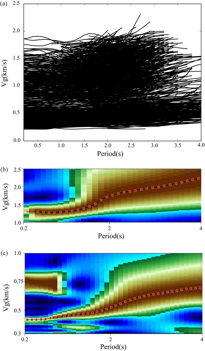
Figure 4. (A) Group velocity dispersion curves in the 0.2–4s period band. (B) Example of interstation (G002-G008) Rayleigh wave group velocity dispersion curve. (C) Example of interstation (G008-G048) Rayleigh wave group velocity dispersion curve. Red asterisks represent the extracted dispersion points.

This study employed a direct surface-wave tomography method to invert all group velocity dispersion curves for the shear-wave velocity structure [19] without the intermediate inversion step for group or phase velocity maps. This method, widely applied in different regions [30–34], employs the fast-marching method proposed for ray tracing to simulate the actual propagation paths of surface waves [35]. It considers that some ray paths will bend away from great-circle paths in the shallow surface based on the fast-marching method [19]. To obtain an optimal model m, this method minimizes differences between the observed travel-times $t_i^{obs}$ and the predicted travel-times $t_i\left(\omega \right)$ calculated from the reference model for all frequencies ω.

$\mathit{\delta }{\mathit{t}}_{\mathit{i}}\left(\mathit{\omega }\right)={\mathit{t}}_{\mathit{i}}^{\mathit{o}\mathit{b}\mathit{s}}-{\mathit{t}}_{\mathit{i}}\left(\mathit{\omega }\right)\approx -{\sum }_{\mathit{k}=\mathbf{1}}^{\mathit{K}}{\mathit{\nu }}_{\mathit{i}\mathit{k}}\frac{\mathit{\delta }{\mathit{C}}_{\mathit{k}}\left(\mathit{\omega }\right)}{{\mathit{C}}_{\mathit{k}}^{\mathbf{2}}\left(\mathit{\omega }\right)}(1)$

where $v_{ik}$ is the bilinear interpolation coefficients along the ray path associated with the ith travel-time data and ${\delta C}_k\left(\omega \right)$ is perturbation of group velocity $C_k\left(\omega \right)$ at the kth 2-D surface grid point at angular frequency ω. Since this method only inverts for shear-wave velocity, it couples the compressional-wave velocity and density with the shear-wave velocity [36]. Thus, Equation (1) can be further transformed to:

$\mathit{\delta }{\mathit{t}}_{\mathit{i}}\left(\mathit{\omega }\right)={\sum }_{\mathit{k}=\mathbf{1}}^{\mathit{K}}\left(-\frac{{\mathit{\nu }}_{\mathit{i}\mathit{k}}}{{\mathit{C}}_{\mathit{k}}^{\mathbf{2}}\left(\mathit{\omega }\right)}\right){\left.{\sum }_{\mathit{j}=\mathbf{1}}^{\mathit{J}}\left[{\mathit{R}}_{\mathit{\alpha }}^{\prime }\left({\mathit{z}}_{\mathit{i}}\right)\frac{\partial {\mathit{C}}_{\mathit{k}}\left(\mathit{\omega }\right)}{\partial {\mathit{\alpha }}_{\mathit{k}}\left({\mathit{z}}_{\mathit{j}}\right)}+{\mathit{R}}_{\mathit{\rho }}^{\prime }\left({\mathit{z}}_{\mathit{i}}\right)\frac{\partial {\mathit{C}}_{\mathit{k}}\left(\mathit{\omega }\right)}{\partial {\mathit{\rho }}_{\mathit{k}}\left({\mathit{z}}_{\mathit{j}}\right)}+\frac{\partial {\mathit{C}}_{\mathit{k}}\left(\mathit{\omega }\right)}{\partial {\mathit{\beta }}_{\mathit{k}}\left({\mathit{z}}_{\mathit{j}}\right)}\right]\right|}_{{\mathit{\theta }}_{\mathit{k}}}\mathit{\delta }{\mathit{\beta }}_{\mathit{k}}\left({\mathit{z}}_{\mathit{j}}\right)={\sum }_{\mathit{l}=\mathbf{1}}^{\mathit{M}}{\mathbf{G}}_{\mathit{i}\mathit{l}}{\mathbf{m}}_{\mathit{l}}(2)$

where $\alpha ,\beta$ and $\rho$ are respectively compressional-wave velocity, mass density, and shear-wave velocity, $\frac{\partial C_k\left(\omega \right)}{\partial {\alpha }_k\left(z\right)},\frac{\partial C_k\left(\omega \right)}{\partial {\beta }_k\left(z\right)}$ and $\frac{\partial C_k\left(\omega \right)}{\partial {\rho }_k\left(z\right)}$ are the group velocity depth sensitivity kernels to them. ${\theta }_k$ denotes the 1-D layered reference model at the kth surface grid point on the surface. $R_{\alpha }^{\prime }$ and $R_{\rho }^{\prime }$ are the scaling factors derived from the empirical relationships [19]. $\delta {\beta }_k\left(z_j\right)$ represents the shear-wave velocity perturbation at the jth depth grid and kth surface grid point. J is the number of grid nodes in the depth direction and M is the total number of grid points in the 3-D model. Equation 2 above gives the final surface wave travel-time perturbation after the discretization of the shear-wave velocity in the depth and horizontal directions.

The average group velocity dispersion curves were used to identify the most reasonable 1D model. We considered it as the initial model to invert the near-surface shear velocity structures. For the inversion grid, the grid interval was 0.0073° along the latitude and 0.0067° along the longitude (which amounts to 18 × 18 grid points). In addition, from 0.2 km to 1.25 km we also placed nine grid points along the depth direction.

Rayleigh wave group velocity values at different periods reflect the characteristics of shear-wave velocity changes within a specific depth range, with the penetration depth increasing as the period lengthens. Therefore, it is necessary to provide sensitivity kernel functions for the group velocities at various depth periods when correlating surface-wave group velocities with S-wave velocities. Figure 5 shows the depth sensitivity kernels for Rayleigh wave group velocities at five periods (0.2, 1.0, 2.0, 3.0, and 4.0 s) and indicates that in the period range of 0.2–4 seconds, our dispersion data can be resolved well down to depths >1.4 km.

Figure 5

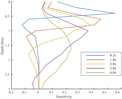
Figure 5. Depth sensitivity kernels for group velocity at 0.2, 1.0, 2.0, 3.0, and 4.0 s.

Figure 6 presents the path coverage of group velocity measurements at four selected periods based on the final 3D velocity model. It can be clearly seen that the path number decreases with the increase of the period. And generally speaking, the ray coverage at these periods is relatively good except for some marginal area, indicating that in the most of the study area, this dataset has the capability to resolve the structure of our study area.

Figure 6

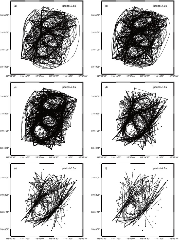
Figure 6. Ray-path coverage for six selected periods (A) 0.5 s, (B) 1.0 s, (C) 2.0 s, (D) 3.0 s, (E) 3.5 s, and (F) 4.0 s. Triangles represent stations, and black lines represent ray paths.

Then a checkerboard resolution test was typically used to evaluate the resolution and errors of data at different depths to test the impact of ray paths and station distribution. This study employed this method to test the reliability of dispersion data, the maximum strength of the shear-wave velocity anomaly was ±50%. With increasing inversion depth, the model resolution gradually decreases (Figure 7). Moreover, Checkerboard models in the middle part of the study area recovered better than the models of the marginal part (Figure 8). Considering that the ray-paths covered more densely in the middle part than in the marginal part of the study area, the checkerboard resolution is generally combined with the ray-path coverage. Owing to the relatively dense data coverage, the velocity anomalies in most of the inversion region can be resolved well.

Figure 7

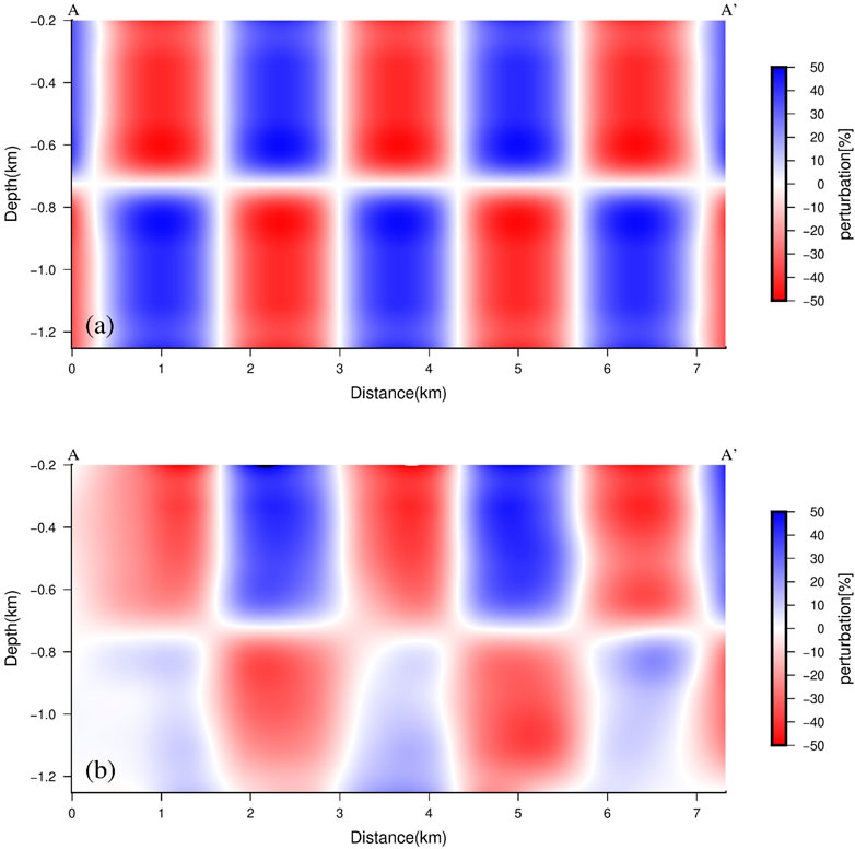
Figure 7. Checkerboard resolution tests in the vertical direction beneath profile AA’ (Figure 2). (A) Initial model, (B) Recovered model.

Figure 8

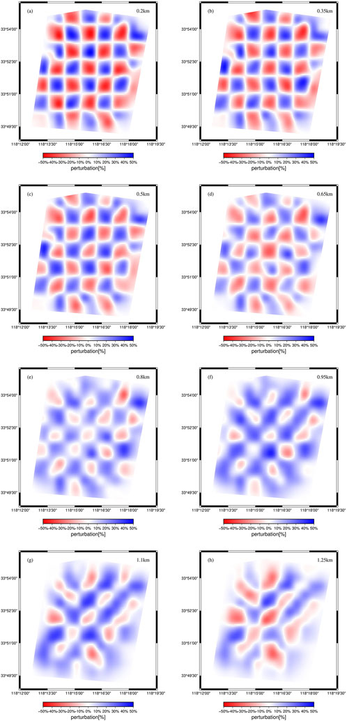
Figure 8. Checkerboard resolution tests of the inversion at depth of (A) 0.20 (B) 0.35, (C) 0.50, (D) 0.65, (E) 0.80, (F) 0.95, (G) 1.1, and (H) 1.25 km.

Finally, we used the group dispersion data in the inversion. Regularization parameters were carefully selected through a trade-off analysis for the inversion [37]. After inversion, the root-mean-square (RMS) residual value decreased from 2.0 s to 1.27 s and remained stable (Figure 9). In the first two iterations, the RMS rapidly reduced. Then it decreased slowly and converged after the 10th iteration, showing that after multiple iterations, the inversion results converged to a stable state.

Figure 9

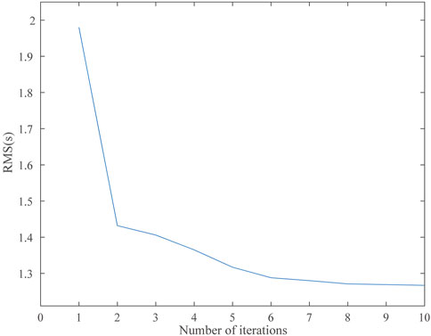
Figure 9. Variation of the RMS value of surface-wave travel-time residuals through the iterations.

3 Results

The S-wave model at different depths is shown in Figure 10. The velocity structure exhibited significant lateral heterogeneity in the study area, with variations in velocity structure at various depths. At a depth of 0.2 km (Figure 10A), the S-wave velocity was generally low, with a spatial distribution showing lower velocities in the eastern area and higher velocities in the western area. In the study area, the depth to the bedrock was approximately 0.28 km, thus the velocity structure at this depth reflected variations in the medium structure of the bottom strata in the Neogene. At 0.35 km depth, velocity anomalies appeared in the study area (Figure 10B), with relatively higher velocities on the west and east sides and a predominance of low velocity anomalies in the middle. Since the depth of 0.2 km is located in the upper part of the bedrock region, the low-velocity anomaly zone in the middle might reflect the development of a fractured zone. At depths >0.65 km (Figures 10D–H), the S-wave velocities showed band-like features, with a west-to-east velocity structure characterized by low-high-low-high-velocity distributions. Based on the development characteristics in the study area, at depths >0.65 km, the high-velocity anomaly in the Daluo region was related to the metamorphic rocks of the Archean-Proterozoic Jiaodong Group (Ar-Pt₂), and the band-like high-velocity anomaly in the Heiyuwang-Nancai area was associated with the Mesozoic Wangshi Formation sandstone (K₂w).

Figure 10

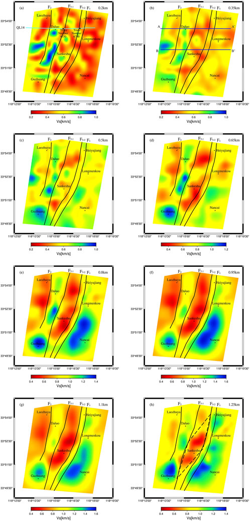
Figure 10. Map view of the shear-wave velocity model at depth of (A) 0.20, (B) 0.35, (C) 0.50, (D) 0.65, (E) 0.80, (F) 0.95, (G) 1.1, and (H) 1.25 km.

4 Discussion

4.1 Spatial distribution and structural characteristics of fault F₅

Using ambient noise tomography, recent studies investigating shallow velocity structures have shown that shallow crustal velocity structures typically correlate well with structural units. For instance, in 3-D S-wave velocity structures, the orientation and location of the significant high- and low-velocity anomalies often match faults passing through the study area [38]. Owing to the evident lateral heterogeneity of S-wave velocities within the study area, we inferred that the distribution of velocity anomalies, combined with previous research on fault distribution characteristics in the Suqian area, can be used to determine the orientation and location of faults within the study area. Based on the S-wave velocity distribution characteristics (Figure 10), it can be inferred that fault F₁ is distributed along the western boundary of the high-velocity anomaly located in the Longmenkou-Nancai area, and fault F₂ is distributed along the eastern boundary of the low-velocity anomaly located in the Laozhuyu area.

A north-south trending low-velocity anomaly zone developed in the Sankeshu area; the eastern and western boundaries of this low-velocity anomaly zone were inferred to be faults F_5-1 and F_5-2, respectively. This low-velocity anomaly is associated with the fractured zone between the two faults. Overall, at least four faults were identified within the study area, namely F₁, F₅ (F_5-1, F_5-2), and F₂, generating a series of NNE trends (Figure 10).

To validate the reasonableness of the inferred fault locations, we compared the results of this study with those of previous studies on fault F₅. Xu et al. (2016) conducted a shallow seismic exploration along the reflection seismic profile QL14 (Figure 11C) [13]. Fault F₅ is composed of multiple-branch faults: fault F_5-1 develops at trace number 4150, fault F_5-2 develops at trace number 6700, and fault F_5-3 develops at trace number 5700. The locations of trace numbers 4150 and 6700 are shown in Figure 10A. By comparing the interpreted locations of faults F_5-1 and F_5-2 from reflection seismic profile QL14 with the fault locations inferred from the map view of the S-wave velocity model, it was observed that the interpretations of faults F_5-1 and F_5-2 from these two profiles were consistent. Therefore, we will subsequently conduct a joint discussion of the results from the QL14 profile and the imaging results presented in this paper. As shown in Figure 11C, the F_5-1 and F_5-2 faults dip towards each other, while the F_5-3 fault is nearly vertical. There are evident fault diffraction waves at the interface of the bedrock and overlying strata along the F_5-3 fault, which is a clear indicator of active faults on the seismic profile. Additionally, the arcuate characteristics of the reflectors within the fault also strongly indicate significant bending and deformation of the strata due to tectonic activity, further confirming the more intense activity of the F_5-3 fault compared to F_5-1 and F_5-2.

Figure 11

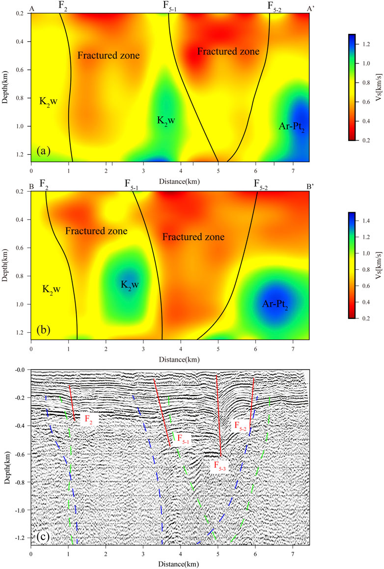
Figure 11. Cross-section of the shear-wave velocity model along (A) AA’ and (B) BB’ and (C) the reflection seismic profile QL14. The red lines represent faults F₂, F_5-1, F_5-2 and F_5-3 shown in the reflection seismic profile QL14, the green dotted lines represent faults F₂, F_5-1 and F_5-2 shown in Figure 11, the blue dotted lines represent faults F₂, F_5-1 and F_5-2 shown in Figure 11.

To better study the fault zone and its velocity structure characteristics, we showed the vertical resolution beneath two profiles traversing the region from west to east, AA’ and BB’ (Figures 11A, B). The locations of these profiles are shown in Figure 10B. Figure 11A shows that fault F₅ is a fault zone composed of two faults, with F_5-1 marked as the western boundary and F_5-2 marked as the eastern boundary. The fractured zone between F_5-1 and F_5-2 exhibited a significant low-velocity anomaly. Faults F_5-1 and F_5-2 likely controlled the Cenozoic depression, which was covered by a thick low-velocity sediment layer. Fault F₅ in the study area comprises two faults that dip in opposite directions, with a deep depression in the middle, consistent with a previous understanding of the distribution characteristics of fault F₅ in the area [10]. Figure 11C shows that a near-vertical fault F_5-3 developed between faults F_5-1 and F_5-2. However, fault F_5-3 is not clearly shown in the AA’ and BB’ profiles, possibly owing to the poor integrity of the rocks within the fractured zone where fault F_5-3 is located and the relatively low transverse velocity heterogeneity. In contrast, the lithological and velocity differences on either side of faults F_5-1 and F_5-2 were more significant, exacerbating the differences in the transverse velocity in the AA’ and BB’ profiles. Hence, the imaging results and the inferred spatial distribution of faults in this study showed a relatively good consistency with those of previous studies. Therefore, subsequent discussions combine the reflection seismic profile QL14 with the imaging results of this study.

The imaging results in this study revealed the development characteristics and spatial distribution of fracture structures within the Neogene (N) and its underlying bedrock (K₂w, Ar). Based on comprehensive shallow seismic exploration results and S-wave velocity imaging, it is found that faults F₁, F₂, and F₅ extended downward to the depth of 1.25 km and below. Faults F_5-1 and F_5-2 collectively controlled a Cenozoic depression with a thick, low-velocity sediment layer. These two boundary faults may merge into a single fracture at greater depths.

4.2 The control of fault F₅ on sediment in the Suqian area

The AA’ profile (Figure 11A) traverses the low-velocity anomaly bodies controlled by faults F₂ and F₅. The boundary characteristics of these low-velocity anomalies were distinct. The orientations of faults F₂, F_5-1, and F_5-2 are highly consistent with the dip directions of the boundaries, each forming a separate low-velocity anomaly center. Among these, the low-velocity anomaly between faults F_5-1 and F_5-2 was more pronounced, extending to depths >1.2 km in the crust, whereas the anomalous body near fault F₂ extended only to approximately 1 km, indicating relatively shallower burial and a smaller extent. Therefore, local sedimentary centers might develop on either side of fault F₂, with a more extensive sedimentary area associated with fault F₅, reflecting the significant control of fault F₅ on the sedimentary thickness of the strata.

The velocity structure along the profiles AA’ and BB’ is consistent with the horizontal velocity structures, revealing a velocity structure which showed low-high-low-high velocity distributions in west-east direction. This suggests that the control of faults on sedimentary layers in the Suqian area does not manifest as an overall uplift or subsidence of the block but rather as differential subsidence. The alternating activity of faults in the Suqian area has formed a tectonic structure characterized by alternating horsts and grabens. Within fault-controlled zones, the sediment in the shallow layers is highly uneven, which could pose challenges for construction projects, necessitating a more detailed geological survey.

4.3 Discussion on the pull-apart basin centered around Sankeshu

Findings from previous research near the Sankeshu area have indicated that three right-stepping faults compose fault F₅, these three faults formed a pull-apart basin which controls the deposition of Neogene and Quaternary strata [13]. Our imaging results indicated that at depths 0.8–1.25 km, the band-like low-velocity anomaly located at Sankeshu diminished with increasing depth. At a depth of 1.25 km, only a portion of the low-velocity anomaly centered around Sankeshu remained (Figure 10H). Combined with our previous conclusion that faults F_5-1 and F_5-2 control a Cenozoic depression with a thick low-velocity sediment layer, this supports the presence of a pull-apart basin and suggests that the basement of the basin lies below 1.25 km. Furthermore, utilizing the map view of the S-wave model (Figure 10) and the reflection seismic profile (Figure 11C), the scale of the pull-apart basin can be roughly determined, as indicated in Figure 10H. The boundary faults of the pull-apart basin are faults F_5-1 and F_5-2, which delineate the western and eastern boundaries of the basin, respectively. In contrast, its northern and southern boundaries correspond to the northern and southern extents of the low-velocity anomaly. Since the reflection seismic profile indicated the presence of reflection wave groups below fault F_5-1, Fault F_5-1 might exert a stronger control over the pull-apart basin, making it the main fault on the eastern edge of the basin. In the early stages, this fault controlled the development of other faults, as well as the formation and evolution of the pull-apart basin.

Fault F_5-3 exhibits the highest activity from the reflection seismic profile, whereas faults F_5-1 and F_5-2 were relatively less active. Based on the positions of these faults within the pull-apart basin and the understanding of similar basins from previous studies [39], we hypothesized that faults F_5-1 and F_5-2 represent early basin-controlling boundary faults and currently show less activity. In contrast, fault F_5-3, located in the central part of the basin, represents a newly developed strike-slip fault, indicating that the recent activity of the pull-apart basin was mainly expressed on this fault, which serves as the main throughgoing fault of this basin.

Given that the extinction of a pull-apart basin commonly manifests as the development of a new strike-slip fault diagonally across the basin [40], we hypothesized that this basin’s latest activity has shifted to the central fault F_5-3. This fault, being an extensional-shear strike-slip, effectively diminishes normal faulting activity along the basin boundary faults as well as within the basin, signalling the basin’s late-stage evolution towards extinction. This transition implies a higher seismic hazard potential for central fault F_5-3. Structurally, the formation and increased activity of the new fault exacerbate seismic risks. Therefore, it is essential to monitor the activity of fault F_5-3 and evaluate its seismic risk. Detailed studies of the geometric characteristics, historical activity, and current stress state of the fault are crucial for developing earthquake disaster prevention and mitigation strategies in the Suqian area.

5 Conclusion

This study utilized continuous vertical component ambient noise waveforms recorded by 100 short-period temporary stations to investigate the shallow crustal structure of the upper crust of fault F₅ in the Suqian area, China. We obtained a 3-D S-wave velocity model for the 0.2–1.25 km depth range in this region. The following results were obtained:

The velocity structure exhibited strong lateral heterogeneity. The development of faults F₁, F₂, and F₅ shows a high degree of consistency with S-wave velocity anomalies. Fault F₅ was composed of two boundary faults F_5-1 and F_5-2, which together controlled a Cenozoic depression covered by a thick low-velocity sediment layer. These two faults might gradually merge into a single fault in the deeper crust.

On either side of fault F₂, localized sedimentary centers have developed. Notably, the sedimentary extent at fault F₅ was relatively larger, which reflected the significant control that fault F₅ exerts over the sedimentary thickness of the strata. The velocity structures along the profiles AA’ and BB’ displayed a low-high-low-high velocity distribution from west to east across the study area. This pattern indicated that the control exerted by the faults over the sedimentary layers in the Suqian region was not manifesting as an overall uplift or subsidence of the block, but rather as differential subsidence. The alternating activity of faults in the Suqian area has formed a tectonic structure characterized by alternating horsts and grabens.

The boundary faults of the pull-apart basin formed by fault F₅ are F_5-1 and F_5-2. Among these two faults, fault F_5-1 served as the primary fault zone on the eastern edge of the basin and has played a dominant role in the development of other faults as well as in the formation and evolution of the entire basin during its early stages, while fault F_5-3 exhibited the highest activity and is a newly developing strike-slip fault within the center of the basin. The latest activity of the pull-apart basin has shifted to fault F_5-3. We hypothesized that its dextral strike-slip movement has decomposed the normal fault activity of the boundary faults, leading to the basin entering a stage of extinction.

Data availability statement

The raw data supporting the conclusions of this article will be made available by the authors, without undue reservation.

Author contributions

QH: Conceptualization, Data curation, Formal Analysis, Investigation, Software, Supervision, Validation, Visualization, Writing–original draft, Writing–review and editing. XF: Data curation, Funding acquisition, Project administration, Software, Supervision, Writing–review and editing. WF: Data curation, Formal Analysis, Software, Supervision, Visualization, Writing–review and editing. PZ: Resources, Supervision, Writing–review and editing. TZ: Supervision, Writing–review and editing. YL: Data curation, Resources, Writing–review and editing. TZ: Data curation, Resources, Writing–review and editing. SR: Data curation, Resources, Writing–review and editing. QW: Data curation, Resources, Writing–review and editing. ZL: Data curation, Resources, Writing–review and editing. TQ: Data curation, Resources, Writing–review and editing.

Funding

The author(s) declare that financial support was received for the research, authorship, and/or publication of this article. This study was supported by the National Natural Science Foundation of China (Grant Nos 42104099 and 41874051).

Conflict of interest

The authors declare that the research was conducted in the absence of any commercial or financial relationships that could be construed as a potential conflict of interest.

Publisher’s note

All claims expressed in this article are solely those of the authors and do not necessarily represent those of their affiliated organizations, or those of the publisher, the editors and the reviewers. Any product that may be evaluated in this article, or claim that may be made by its manufacturer, is not guaranteed or endorsed by the publisher.

References

1. Zhu G, Wang D, Liu G, Song C, Xu J, Niu M. Extensional activities along the Tan-Lu fault zone and its geodynamic setting. Chin J Geol (2001) 36:269–78.

Google Scholar

2. Deng Y, Fan W, Zhang Z, Badal J. Geophysical evidence on segmentation of the Tancheng-Lujiang fault and its implications on the lithosphere evolution in East China. J Asian Earth Sci (2012) 78:263–76. doi:10.1016/j.jseaes.2012.11.006

CrossRef Full Text | Google Scholar

3. Zhang H, Li L, Jiang X, Zhang D, Xu H. New progress in paleoearthquake studies of the Jiangsu segment of the Anqiu-Juxian Fault in the Tanlu fault zone. Seismol Geol (2023) 45:880–95. doi:10.3969/j.issn.0253-4967.2023.04.005

CrossRef Full Text | Google Scholar

4. Chao HT, Li J, Cui Z, Zhao Q. Discussion on several problems related to the seismic fault of the 1688 Tancheng earthquake (M= 8½). North China Earthquake Sci (1997) 15:18–25.

Google Scholar

5. Shi W, Zhang Y, Dong S. Quaternary activity and segmentation behavior of the middle portion of the Tan-Lu fault zone. Acta Geosci Sin (2003) 24:11–8.

Google Scholar

6. Liu B, Feng S, Ji J, Shi J, Tan Y, Li Y. Fine lithosphere structure beneath the middle-southern segment of the Tan-Lu fault zone. Chin J Geophys (2015) 58:1610–21. doi:10.6038/cjg20150513

CrossRef Full Text | Google Scholar

7. Wang H, Geng J. Some features of 1668 Tancheng earthquake (M= 8½) fault. North China Earthquake Sci (1992) 10:34–42.

Google Scholar

8. Chao H, Li J, Cui Z, Zhao Q. Characteristic slip behavior of the Holocene fault in the central section of the Tan-Lu fault zone and the characteristic earthquakes. Inland Earthquake (1994) 8:297–30.

Google Scholar

9. Li J, Chao H, Cui Z, Zhao Q. Segmentation of active fault along the Tancheng-Lijiang fault zone and evaluation of strong earthquake risk. Seismol Geol (1994) 16:121–6.

Google Scholar

10. Zhang P, Li L, Ran Y, Cao J, Xu H, Jiang X. Research on characteristics of late quaternary activity of the Jiangsu segment of Anqiu-Juxian fault in the Tanlu fault zone. Seismol Geol (2015) 37:1162–76. doi:10.3969/j.issn.0253-4967.2015.04.018

CrossRef Full Text | Google Scholar

11. Zhang P, Zhang Y, Li L, Jiang X, Meng K. New evidences of Holocene activity in the Jiangsu segment of Anqiu-Juxian fault of the Tanlu fault zone. Seismol Geol (2019) 41:576–86. doi:10.3969/j.issn.0253-4967.2019.03.003

CrossRef Full Text | Google Scholar

12. Zhang P, Li L, Zhang J, Jiang W, Chen D, Li J, et al. A discuss of the characteristics of activities in quaternary for the Jiangsu segment of Tan-Lu fault zone and its geodynamic setting. J Disaster Prev Mitigation Eng (2011) 31:389–96. doi:10.3969/j.issn.1672-2132.2011.04.007

CrossRef Full Text | Google Scholar

13. Xu H, Fan X, Ran Y. New evidences of the Holocene fault in Suqian segment of the Tanlu fault zone discovered by shallow seismic exploration method. Seismol Geol (2016) 38:31–43. doi:10.3969/j.issn.0253-4967.2016.01.003

CrossRef Full Text | Google Scholar

14. Cao J, Ran Y, Xu H, Li Y, Zhang P, Ma X, et al. Typical case analysis on application of multi-method detection technique to active fault exploration in Suqian city. Seismol Geol (2015) 37:430–9. doi:10.3969/j.issn.0253-4967.2015.02.007

CrossRef Full Text | Google Scholar

15. Meng Y, Yao H, Wang X, Li L, Feng J, Hong D, et al. Crustal velocity structure and deformation features in the central-southern segment of Tanlu fault zone and its adjacent area from ambient noise tomography. Chin J Geophys (2019) 62:2490–509. doi:10.6038/cjg2019M0189

CrossRef Full Text | Google Scholar

16. Qin J, Liu B, Xu H, Shi J, Tan Y, He Y, et al. Exploration of shallow structural characteristics in the Suqian segment of the TanLu fault zone based on seismic refraction and reflection method. Chin J Geophys (2020) 63:505–16. doi:10.6038/cjg2020N0144

CrossRef Full Text | Google Scholar

17. Sabra KG, Gerstoft P, Roux P, Kuperman WA, Fehler MC. Surface wave tomography from microseisms in Southern California. Geophys Res Lett (2005) 32:L14311. doi:10.1029/2005GL023155

CrossRef Full Text | Google Scholar

18. Yao H, Van Der Hilst RD, De Hoop MV. Surface-wave array tomography in SE Tibet from ambient seismic noise and two-station analysis—I. Phase velocity maps. Geophys J Int (2006) 166:732–44. doi:10.1111/j.1365-246X.2006.03028.x

CrossRef Full Text | Google Scholar

19. Fang H, Yao H, Zhang H, Huang Y, Van Der Hilst RD. Direct inversion of surface wave dispersion for three-dimensional shallow crustal structure based on ray tracing: methodology and application. Geophys J Int (2015) 201:1251–63. doi:10.1093/gji/ggv080

CrossRef Full Text | Google Scholar

20. Zhou L, Xie J, Shen W, Zheng Y, Yang Y, Shi H, et al. The structure of the crust and uppermost mantle beneath South China from ambient noise and earthquake tomography. Geophys J Int (2012) 189:1565–83. doi:10.1111/j.1365-246X.2012.05423.x

CrossRef Full Text | Google Scholar

21. Li C, Yao H, Fang H, Huang X, Wan K, Zhang H, et al. 3D near-surface shear-wave velocity structure from ambient noise tomography and borehole data in the Hefei urban area, China. Seismol Res Lett (2016) 87:882–92. doi:10.1785/0220150257

CrossRef Full Text | Google Scholar

22. Yao H, Gouédard P, Collins JA, McGuire JJ, Van Der Hilst RD. Structure of young East Pacific Rise lithosphere from ambient noise correlation analysis of fundamental- and higher-mode Scholte-Rayleigh waves. C R Géoscience (2011) 343:571–83. doi:10.1016/j.crte.2011.04.004

CrossRef Full Text | Google Scholar

23. Lin F, Li D, Clayton RW, Hollis D. High-resolution 3D shallow crustal structure in Long Beach, California: application of ambient noise tomography on a dense seismic array. Geophysics (2013) 78:Q45–Q56. doi:10.1190/geo2012-0453.1

CrossRef Full Text | Google Scholar

24. Chmiel M, Mordret A, Boue P, Brenguier F, Lecocq T, Courbis R, et al. Ambient noise multimode Rayleigh and Love wave tomography to determine the shear velocity structure above the Groningen gas field. Geophys J Int (2019) 218:1781–95. doi:10.1093/gji/ggz237

CrossRef Full Text | Google Scholar

25. Gu N, Wong N, Gao J, Ding N, Yao H, Zhang H. Shallow crustal structure of the Tanlu Fault Zone near Chao Lake in eastern China by direct surface wave tomography from local dense array ambient noise analysis. Pure Appl Geophys (2019) 176:1193–206. doi:10.1007/s00024-018-2041-4

CrossRef Full Text | Google Scholar

26. Wei Z, Chu R, Chen L, Wu S. Crustal structure in the middle-southern segments of the Tanlu Fault Zone and adjacent regions constrained by multifrequency receiver function and surface wave data. Phys Earth Planet Inter (2020) 301:106470. doi:10.1016/j.pepi.2020.106470

CrossRef Full Text | Google Scholar

27. Bensen GD, Ritzwoller MH, Barmin MP, Levshin AL, Lin F, Moschetti MP, et al. Processing seismic ambient noise data to obtain reliable broad-band surface wave dispersion measurements. Geophys J Int (2007) 169:1239–60. doi:10.1111/j.1365-246X.2007.03374.x

CrossRef Full Text | Google Scholar

28. Zhang Y, Yao H, Yang H, Cai H, Fang H, Xu J, et al. 3-D crustal shear-wave velocity structure of the Taiwan Strait and Fujian, SE China, revealed by ambient noise tomography. JGR Solid Earth (2018) 123:8016–31. doi:10.1029/2018JB015938

CrossRef Full Text | Google Scholar

29. Yao H, Van Der Hilst RD. Analysis of ambient noise energy distribution and phase velocity bias in ambient noise tomography, with application to SE Tibet. Geophys J Int (2009) 179:1113–32. doi:10.1111/j.1365-246X.2009.04329.x

CrossRef Full Text | Google Scholar

30. Huang Y, Yao H, Huang B, Van Der Hilst RD, Wen K, Huang W, et al. Phase velocity variation at periods of 0.5–3 seconds in the Taipei Basin of Taiwan from correlation of ambient seismic noise. Bull Seismol Soc Am (2010) 100:2250–63. doi:10.1785/0120090319

CrossRef Full Text | Google Scholar

31. Liu C, Yao H, Yang H, Shen W, Fang H, Hu S, et al. Direct inversion for three-dimensional shear wave speed azimuthal anisotropy based on surface wave ray tracing: methodology and application to Yunnan, southwest China. JGR Solid Earth (2019) 124:11394–413. doi:10.1029/2018JB016920

CrossRef Full Text | Google Scholar

32. Gu Q, Ding Z, Kang Q, Li D. Group velocity tomography of Rayleigh wave in the middle-southern segment of the Tan-Lu fault zone and adjacent regions using ambient seismic noise. Chin J Geophys (2020) 63:1505–22. doi:10.6038/cjg2020N0117

CrossRef Full Text | Google Scholar

33. Luo S, Yao H, Li Q, Wang W, Wan K, Meng Y, et al. High-resolution 3D crustal S-wave velocity structure of the Middle-Lower Yangtze River Metallogenic Belt and implications for its deep geodynamic setting. Sci China Arth Sci (2019) 62:1361–78. doi:10.1007/s11430-018-9352-9

CrossRef Full Text | Google Scholar

34. Zheng L, Fan X, Zhang P, Hao J, Qian H, Zheng T. Detection of urban hidden faults using group-velocity ambient noise tomography beneath Zhenjiang area, China. Sci Rep (2021) 11:987. doi:10.1038/s41598-020-80249-6

PubMed Abstract | CrossRef Full Text | Google Scholar

35. Rawlinson N, Sambridge M. Wave front evolution in strongly heterogeneous layered media using the fast marching method. Geophys J Int (2004) 156:631–47. doi:10.1111/j.1365-246X.2004.02153.x

CrossRef Full Text | Google Scholar

36. Brocher TM. Empirical relations between elastic wavespeeds and density in the Earth’s crust. Bull Seismol Soc Am (2005) 95:2081–92. doi:10.1785/0120050077

CrossRef Full Text | Google Scholar

37. Aster RC, Borchers B, Thurber CH. Parameter estimation and inverse problems. 2nd ed. Academic (2013).

Google Scholar

38. Jin J, Luo S, Yao H, Tian X. Dense array ambient noise tomography reveals the shallow crustal velocity structure and deformation features in the Weifang segment of the Tanlu fault zone. Chin J Geophys (2023) 66:558–75. doi:10.6038/cjg2022P0934

CrossRef Full Text | Google Scholar

39. Shu P, Xu X, Feng S, Liu B, Li K, Tapponnier P, et al. Sedimentary and tectonic evolution of the Banquan pull-apart basin and implications for Late Cenozoic dextral strike-slip movement of the Tanlu Fault Zone. Sci China (Earth Sci.) (2023) 66:797–820. doi:10.1007/s11430-022-1028-5

CrossRef Full Text | Google Scholar

40. Zhang P, Burchfiel BC, Chen S, Deng Q. Extinction of pull-apart basins. Geology (1989) 17:814–7. doi:10.1130/0091-7613(1989)017<0814:eopab>2.3.co;2

CrossRef Full Text | Google Scholar