Hyperboloidal method for quasinormal modes of non-relativistic operators

The recently reported compactified hyperboloidal method has found wide use in the numerical computation of quasinormal modes, with implications for fields as diverse as gravitational physics and optics. We extend this intrinsically relativistic method into the non-relativistic domain, demonstrating its use to calculate the quasinormal modes of the Schrödinger equation and solve related bound-state problems. We also describe how to further generalize this method, offering a perspective on the importance of non-relativistic quasinormal modes for the programme of black hole spectroscopy.

Introduction

Quasinormal modes (QNMs) are complex frequency modes which characterize the resonant response of a system to linear perturbations. They are prevalent in the physics of waves, with special prominence in optics and gravitational physics. In optics, QNMs are useful for understanding the behaviour of resonant photonic structures, such as plasmonic crystals, nanoparticle traps, metal gratings, and optical sensors [1–5]. In gravitational physics, they are thought relevant to tests of black hole no-hair conjectures [6–8], and central to the emerging project of black hole spectroscopy with gravitational waves [9, 10]. While the QNM literature in optics treats dispersion as a matter of necessity [11, 12], the prevailing methods in gravitational physics are concerned with non-dispersive, relativistic wave propagation [13–15]. We believe there are good reasons to go beyond relativistic wave propagation in the gravitational context. A variety of quantum gravity models predict the dispersive propagation of gravitational waves [16–19], for example, in models with a non-zero graviton mass, violation of Lorentz invariance, and higher dimensions [20–22]. Indeed, it has been proposed that QNMs may be used to probe gravity beyond general relativity, through imprints on radiative emission from black holes [23–27]. More generally, we anticipate that developments of QNM methods for non-relativistic operators will broaden the scope of existing questions in QNM theory.

Numerical methods underpin much of the progress in QNMs over recent years. Indeed, efficient schemes for computing the QNMs of potentials are likely indispensable for future developments in both theory and the modelling of observations. Recently, the so-called compactified hyperboloidal method [28–31] has proven to be a powerful tool, finding wide use in the computation of black hole QNM spectra and bringing within reach the systematic exploration of their connection to pseudospectra [32–39]. Beyond this, it is natural to ask whether the method can also find use in optical systems. We believe it can, but it cannot be widely applied in optics without modification. This is because optical media create non-relativistic and dispersive dynamics, while the present formulation of the method treats only relativistic and non-dispersive dynamics, as may be seen from its use of hyperbolic spatial slices penetrating the black hole horizon and future null infinity.

A notable optical system that motivates the development of a hyperboloidal method for optics is the fiber optical soliton, which has recently been established as a black hole analogue with an exactly known QNM spectrum [40]. As such, the soliton is the ideal system with which to develop the method, as the resulting numerics can be compared both to known analytical results and to the numerics of the corresponding relativistic system. Moreover, perturbations to the soliton realize the Schrödinger equation with a Pöschl-Teller potential, making the soliton a promising experimental platform with which to address questions in QNM theory, such as the physical status of spectral instabilities observed in QNM numerics, where the Pöschl-Teller potential is paradigmatic [30, 41–44].

In this article, we outline a new method for the numerical computation of QNM spectra for operators with a non-relativistic dispersion relation, by adapting the compactified hyperboloidal method. We begin by showing how to compute the QNMs of the Schrödinger equation for an arbitrary potential, noting that the relativistic and non-relativistic spectra are related by a simple endomorphism. We subsequently demonstrate the method for the Pöschl-Teller potential, explicitly calculating the soliton QNM spectrum numerically. Finally, we sketch how to develop these ideas in order to treat generalized non-relativistic dispersion relations, and discuss potential applications of the more general method, with emphasis on its future use in black hole spectroscopy.

Compactified hyperboloidal method for the Schrödinger equation

We begin by considering a scalar field $\varphi$ which obeys a Schrödinger equation of the form,

$\left(i{\partial }_t-{\partial }_r^2+V\right)\varphi =0,(1)$

with $V$ a potential that vanishes for $r\to \pm \infty$. The boundary conditions for QNMs describe solutions that transport energy away from the potential, as discussed in more detail in [40]. It can be shown, using the asymptotic dispersion relation of Equation 1, that QNM solutions must diverge for $r\to \pm \infty$. That is, the asymptotic form of the solution must be $\varphi \sim \exp (iKr-i\mathrm{\Omega }t)$, with the requirement that $\text{Im}(K)$ is positive and negative on the left and right, respectively. These spatial divergences are problematic for numerical methods, but they can be removed by using a hyperboloidal coordinate transformation. Following [30], we adopt coordinates,

$t=\tau -h\left(x\right),r=g\left(x\right),(2)$

where $g(x),h(x)$ are yet to be given, and ${\partial }_{\tau }={\partial }_t$ by construction. In the relativistic context, these are used to compute QNMs of black holes, with $h(x)$ chosen so that contours of $\tau$ tend to null curves that intersect the horizon and future null infinity. There, Equation 2 is intended to respect the asymptotic hyperbolic geometry of the spacetime, giving rise to bounded and well-behaved QNM solutions. However, there is no preferred speed in our non-relativistic system, meaning that no coordinate transformation will consistently give rise to bounded solutions. This requires a different approach.

In order to construct bounded QNM solutions, we first parameterize $h(x)$ by a new variable $v_g$ such that contours of $\tau$ tend asymptotically to trajectories directed outwards with $|dr/dt|=v_g$. In particular, we write

$g\left(x\right)=\text{arctanh}x,h\left(x\right)={\left(2v_g\right)}^{-1}\log \left(1-x^2\right),(3)$

where $g(x)$ compactifies the space such that the real line of $r$ gives $x\in [-\mathrm{1,1}]$ if we close the set by including the boundaries. In the Supplementary Appendix, we show that QNMs whose asymptotic group velocity is $v_g$ in $(r,t)$ coordinates are finite at the spatial boundaries, $x=\pm 1$. This enforces the boundary conditions for these modes, but does not guarantee that any such modes exist.

In contrast to the relativistic case, dispersion in non-relativistic systems means that group and phase velocities are not the same. As a result, QNMs whose asymptotic phase velocity is $v_p\ne v_g$ in $(r,t)$ coordinates will undergo phase divergences at the boundaries. This can be removed by a phase-rotation of the field,

$\widehat{\varphi }=e^{-\mathrm{\Delta }\log \left(1-x^2\right)/2}\varphi ,(4)$

where we introduce $\mathrm{\Delta }=i(v_g-v_p)/2$, so that the phase rotation is parameterized by both $v_g$ and $v_p$. The form of the required phase rotation follows from the asymptotic dispersion relation of Equation 1 and the choice of height function, $h(x)$. Intuitively, it depends on the mismatch of the two velocities. The result is that the field $\widehat{\varphi }$ is bounded and well-defined on the new space.

The cost of the above construction is that we introduce two unknown real parameters, $v_g$ and $v_p$, into the problem. In fact, identifying velocity pairs that correspond to actual QNM solutions is as difficult a problem as determining the QNM spectrum itself. This may be seen by the relation,

$\mathrm{\Omega }=-\frac{1}{2}{v}_g\left(v_p+i\sqrt{v_g\left(v_g-2v_p\right)}\right),(5)$

which we derive, in the Supplementary Appendix, from the asymptotic dispersion relation of Equation 1. This holds true for any mode whose asymptotic group and phase velocities are $v_g$ and $v_p$, respectively. The existence of a relation such as Equation 5 is a direct consequence of dispersion. In a relativistic system, all asymptotic speeds are the speed of light, so $\mathrm{\Omega }$ cannot be expressed in terms of asymptotic velocities. This difference between the relativistic and non-relativistic methods is crucial. Equations 3, 4 mean we obtain an equation of motion, and an eigenvalue equation for the complex frequency $\mathrm{\Omega }$, both of which are parameterized by $v_g$ and $v_p$. The significance of Equation 5 is that these additional parameters can ultimately be eliminated, leaving $\mathrm{\Omega }$ as the only unknown in the problem.

We proceed as in [30], by rewriting Equation 1 in the new coordinates and performing a first-order reduction in time, introducing the auxiliary field $\widehat{\psi }$. The equation of motion becomes ${\partial }_{\tau }\widehat{\varphi }=\widehat{\psi }$ with

$x^2{\partial }_{\tau }\widehat{\psi }=J_1\widehat{\varphi }+J_2\widehat{\psi },(6)$

where $J_1$ and $J_2$, given in the Supplementary Appendix, are spatial operators depending on the potential and the asymptotic velocities. In contrast to the relativistic method, ${\partial }_{\tau }\widehat{\psi }$ cannot be isolated by division in Equation 6 because its pre-factor vanishes at $x=0$. This occurs because the contours of $\tau$ have to “turn around” in order to be outgoing in the $(r,t)$ coordinates. Our alternative approach is to construct ${\partial }_{\tau }\widehat{\psi }$ using a Taylor series around $x=0$, obtaining the required derivatives by repeated differentiation of Equation 6. In fact, this treatment is necessary only for terms indivisible by $x^2$, and we obtain a simpler result if we initially separate the terms in this way. This separation is mostly trivial, but for the potential, where we write $V=V_0+x{V}_1+x^2\tilde{V}(x)$, with $V_0$ and $V_1$ Taylor series coefficients about $x=0$ and $\tilde{V}$ accounting for the remaining terms. We obtain

${\partial }_{\tau }\widehat{\psi }=L_1\widehat{\varphi }+L_2\widehat{\psi },(7)$

where $L_1$ and $L_2$ are spatial operators that we derive in the Supplementary Appendix. Equation 7 is formally identical to that obtained in the relativistic method [30], but the operators are quite different, containing arbitrarily high spatial derivatives and depending on the asymptotic velocities.

In matrix form, we write $i{\partial }_{\tau }u=Lu$ with

$u\equiv \left(\begin{array}{c}\hfill \widehat{\varphi }\hfill \\ \hfill \widehat{\psi }\hfill \end{array}\right),L\equiv i\left(\begin{array}{cc}\hfill 0\hfill & \hfill 1\hfill \\ \hfill L_1\hfill & \hfill L_2\hfill \end{array}\right),$

and obtain the mode equation

$Lu=\mathrm{\Omega }u.(8)$

The operator $L$ is parameterized by $v_g$ and $v_p$, giving rise to a family of operators. For each operator, Equation 8 defines a unique eigenvalue problem and a corresponding spectrum. However, only a subset of the frequencies from these spectra obey Equation 5, and it is this subset which comprises the QNM spectrum of Equation 1. Using Equation 5 to eliminate $v_g$ and $v_p$, one obtains a problem in which the frequency $\mathrm{\Omega }$ is the only unknown and all solutions correspond to QNMs. In this formulation, $L$ is parameterized by $\mathrm{\Omega }$, which constitutes an essential difference from the relativistic method, wherein the corresponding operator does not depend on $\mathrm{\Omega }$ [30]. Importantly, Equation 8 unambiguously determines the QNM spectrum.

Equation 8 is discretized using $N$-point Chebyshev nodes of the second kind. In this way, fields are approximated by $N$-dimensional vectors and spatial operators by $N$-dimensional matrices. It follows that the vector $u$ and the operator $L$ are approximated by $2N$-dimensional vectors and matrices, respectively. The result is

$L^N{u}^N=\mathrm{\Omega }{u}^N.(9)$

The QNM spectrum may then be obtained from Equation 9 in the usual way using $\det (L^N-\mathrm{\Omega }\text{Id})=0$. In the Supplementary Appendix, we show that this determinant may be rewritten as that of a smaller $N$-dimensional matrix, $M$. Its elements are quadratic in the square root of the QNM frequency, giving rise to a polynomial of degree $2N$ in $\sqrt{\mathrm{\Omega }}$. For a given potential $V$, the roots may be numerically determined in order to give $2N$ of the QNM frequencies. The fact that the frequency enters via its square root is a result of the Schrödinger equation having a first derivative in time, rather than a second derivative in time like the wave equation. Indeed, the exact QNM spectra of the Schrödinger and wave equations are related to each other by $i\sqrt{\mathrm{\Omega }}=\omega$, as was elaborated in [40]. This means we can relate the results of the non-relativistic method to those of the relativistic method, allowing us to better evaluate the accuracy of the new method.

Quasinormal modes of the Pöschl-Teller potential

In this section, we use the above numerical method to calculate the QNMs of the Schrödinger equation with the Pöschl-Teller potential,

$V=V_0{\text{sech}}^2\left(r\right)=V_0\left(1-x^2\right),(10)$

which serves as an exemplar for both the relativistic and non-relativistic methods. The QNMs of Equation 10 are finite polynomials in the compactified spatial coordinate, with the result that an $N$-point discretization reproduces the first $2N$ QNMs to arbitrary precision. The Pöschl-Teller potential is also ideal because the corresponding QNM spectrum of the Schrödinger equation is given analytically by

${\mathrm{\Omega }}_n={\left[n+\frac{1}{2}-i\sqrt{V_0-\frac{1}{4}}\right]}^2,(11)$

allowing us to verify our results [40]. In regards to the non-relativistic method, we note that the Pöschl-Teller potential is especially simple because all its QNMs have the same $v_g$ parameter, which is a result of the fact that $i\sqrt{\mathrm{\Omega }}$ is aligned along vertical lines in the complex plane for this potential. While this simplicity does not influence the operation of the method, it does allow us to more easily assess the spectrum. Lastly, we partition the Pöschl-Teller potential with $V_1=0$ and $\tilde{V}=-V_0$, which reinforces the simplicity of the potential.

Now, we make some comments on the specifics of our implementation of the method. We find the calculation is significantly more efficient for odd $N$. This is a consequence of discretization. The Taylor series expansions of $L_1$ and $L_2$ involve spatial derivatives at $x=0$, which are obtained by integration with a Dirac delta function in the continuous case, and by matrix multiplications in the discretized case. For odd $N$, the relevant matrix is zero everywhere but a central column whose entries are unity. However, for even $N$, the matrix is everywhere populated, and this increases the computational cost of the calculation. We also find that evaluating the determinant of the large symbolic matrix $M$ is inefficient, so we instead sample the determinant in the complex plane and reconstruct the symbolic determinant using polynomial interpolation. This uses that the method produces a polynomial of degree $2N$ in $\sqrt{\mathrm{\Omega }}$. Importantly, this is true no matter what potential we consider.

In Figure 1A, we plot the exact QNM frequencies of the unperturbed Pöschl-Teller potential, given in Equation 11 [40] alongside those calculated by the new numerical method, with a resolution of $N=201$. We find excellent agreement for all frequencies, with an error which may be made arbitrarily small by increasing the working precision. These results are given in Figure 2. We also calculate the QNM spectrum of a perturbed Pöschl-Teller potential,

$V=V_0\left(1-x^2\right)+ϵ\mathrm{\Delta }V,(12)$

where $ϵ=10^{-30}$ and $\mathrm{\Delta }V$ is a randomly chosen polynomial of degree 9, shown in the inset of Figure 1. We find that the spectrum for Equation 12 closely resembles the unperturbed spectrum up to the $10^{\text{th}}$ overtone index, beyond which the frequencies are significantly displaced from their unperturbed values, as shown in Figure 2. These numerical results are then indicative of spectral instabilities that have been reported by previous authors [30, 45, 46].

Figure 1

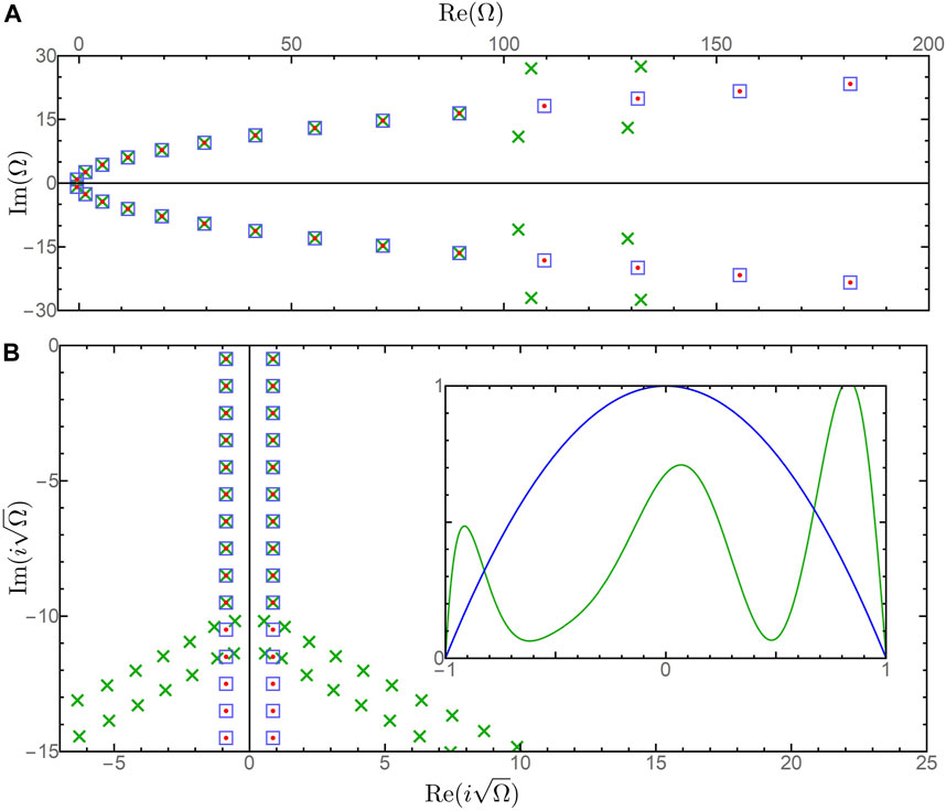
Figure 1. QNM spectra for the Schrödinger equation with a potential $V=V_0{\text{sech}}^2(r)+ϵ\mathrm{\Delta }V$, where $V_0=1$ and $\mathrm{\Delta }V$ is the perturbation shown in green in the inset, alongside the unperturbed Pöschl-Teller potential in blue. The red dots and blue boxes correspond to the unperturbed Pöschl-Teller potential $(ϵ=0)$, with red dots ( ) given by the exact formula and blue boxes ( ) numerically determined by the new method. The green crosses ( ) correspond to a perturbed potential $(ϵ=10^{-30})$ and are also numerically determined. (A) Displays the three QNM spectra, while (B) Displays the same spectra under the transformation $\mathrm{\Omega }\to i\sqrt{\mathrm{\Omega }}$, which relates the spectra to those of a corresponding relativistic operator.

Figure 2

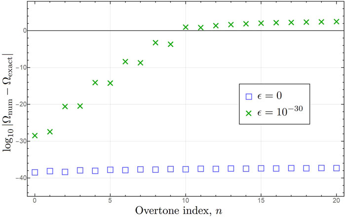
Figure 2. Comparisons of exact and numerically determined QNM frequencies for the Schrödinger equation with a potential $V=V_0{\text{sech}}^2(r)+ϵ\mathrm{\Delta }V$, where $V_0=1$ and $\mathrm{\Delta }V$ is the perturbation shown in Figure 1. The first 21 QNM frequencies are displayed. The unperturbed $(ϵ=0)$ spectrum is recovered well by the new numerical method, with errors smaller than $10^{-37}$ for the chosen working precision. We also obtain the perturbed $(ϵ=10^{-30})$ spectrum and find the deviation from the exact spectrum grows rapidly with overtone index, $n$, as in previous works on spectral instability.

The simple relationship between the QNMs of the Schrödinger and wave equations becomes visible under the transformation $\mathrm{\Omega }\to i\sqrt{\mathrm{\Omega }}$, which maps the spectrum of the former onto that of the latter. In Figure 1B, we plot $i\sqrt{\mathrm{\Omega }}$ for the same spectra as above, obtaining the recognizable vertical lines in the complex plane that are characteristic of the wave equation with a Pöschl-Teller potential. In this way, we illustrate how one can cross-verify the results of the relativistic and non-relativistic methods against each other, for arbitrary potentials.

Discussion

In this section, we discuss potential applications of the non-relativistic compactified hyperboloidal method that we developed in the preceding text, suggesting well-motivated directions in which to further develop the method and providing a sketch of how this can be achieved. The main motivations for this method were the modelling of QNMs of optical solitons, and the development of a framework within which one can treat QNMs in quantum gravity models with dispersive gravitational wave propagation. Beyond these, we note that this non-relativistic method may be employed equally well in any system governed by a Schrödinger equation equipped with a general potential. In this paper, we numerically calculated QNM spectra for the Pöschl-Teller potential and perturbations of that potential, finding agreement with earlier works [40, 47, 50]. For potentials with different long-range behaviour than the Pöschl-Teller potential, one typically requires different choices of height function $h(x)$, but this requirement is shared by the relativistic method, and may be addressed by the same techniques [29, 48, 49]. In addition, we note that this method may also be used to numerically solve for the quantum mechanical bound-states of a general potential well, using the well-known connection between the QNMs of a potential barrier and the bound-states of the corresponding well [41, 51–53].

As described above, the non-relativistic method we have presented is closely related to the relativistic method, sharing many essential features with it. For instance, the classes of potentials that can be treated by the two methods are the same, and they have the same maximum achievable accuracy for a given resolution. As a result, the methods are comparable in their scope and power. They also share the same advantages and disadvantages when compared to other popular numerical methods, such as Leaver’s continued fraction method [54]. For example, in this case, both the relativistic and non-relativistic methods enjoy the advantage that they recover the entire spectrum simultaneously, and do not require initial seed values close to the QNM frequencies one wishes to compute [30, 54–56].

The non-relativistic method we have presented readily generalizes beyond the Schrödinger equation, allowing us to treat a large class of more general non-relativistic operators. Indeed, the method presented in this paper primarily serves a didactic purpose, as a demonstration of a general approach with which one may calculate QNMs of these more general operators. The primary motivation for this is to facilitate the efficient computation of QNMs of operators that deviate from the wave equation only by the presence of weak dispersion, as are known to arise in models of quantum gravity, where a thoroughgoing understanding of QNMs is of special interest. The modelling of dispersive gravitational wave propagation and its influence on the observable QNM spectrum will be essential if black hole spectroscopy is to be an effective probe into the domain of quantum gravity.

A further motivation for generalizing the non-relativistic method is to shed light on QNM spectral instabilities, and facilitate experimental tests of the recent ultraviolet universality conjecture, which posits that sufficiently high overtones converge to logarithmic Regge branches in the complex plane, in the high-frequency limit of potential perturbations [30, 36]. This effect is easily seen in numerical calculations of the Pöschl-Teller spectrum, on account of its simplicity, but has yet to be experimentally confirmed. Using the optical soliton, whose perturbations realize this potential, experimental tests become possible. The numerical method presented above is essential for the modelling of these experiments, as one cannot realize an exact soliton in practice, and must always work with near-soliton potentials. In addition, higher-order dispersive effects will also be present in any experiment, and these must be understood in order to interpret observations of QNM spectral migration with the soliton. In particular, the influence of weak third-order dispersion acting on the perturbative probe field should be incorporated into the analysis, in order to provide the best test of the above conjecture. This motivates the development of the non-relativistic method beyond the Schrödinger equation, to include higher-order dispersive terms.

In view of the above reasons to generalize the non-relativistic method, we present a sketch of the more general method, which we will elaborate in future work. Suppose we have a non-relativistic equation of the form

$\left(\alpha \left(i{\partial }_t\right)+\beta \left(i{\partial }_r\right)+V\right)\varphi =0,(13)$

with $\alpha (z)$ and $\beta (z)$ finite polynomials in $z$, and $d$ the larger degree among the two polynomials. In principle, we can apply a hyperboloidal coordinate transformation and a phase rotation of the fields, parameterised by the asymptotic velocities, $v_g$ and $v_p$. Then, we introduce auxiliary fields to effect a $d$th-order reduction in time, defining

${\varphi }_1=\varphi ,{\varphi }_{k+1}={\partial }_{\tau }{\varphi }_k,(14)$

with $1\le k<d$. Equation 14 closely mirrors the treatment of resonator QNMs in optics [11]. The equations of motion of these fields are trivial for all fields but ${\varphi }_d$, whose equation of motion more closely resembles Equation 6. If we use a Taylor series expansion of ${\partial }_{\tau }{\varphi }_d$ around zero, we can write it in terms of spatial operators acting on the fields. The general form of the now $d$-dimensional operator $L$ is

$L=\left(\begin{array}{ccccc}\hfill 0\hfill & \hfill 1\hfill & \hfill 0\hfill & \hfill \cdots \hfill & \hfill 0\hfill \\ \hfill 0\hfill & \hfill 0\hfill & \hfill 1\hfill & \hfill \cdots \hfill & \hfill 0\hfill \\ \hfill 0\hfill & \hfill 0\hfill & \hfill 0\hfill & \hfill \cdots \hfill & \hfill 0\hfill \\ \hfill ⋮\hfill & \hfill ⋮\hfill & \hfill ⋮\hfill & \hfill \ddots \hfill & \hfill 1\hfill \\ \hfill L_1\hfill & \hfill L_2\hfill & \hfill L_3\hfill & \hfill \cdots \hfill & \hfill L_d\hfill \end{array}\right),(15)$

which we discretize as before. Then, we use the asymptotic dispersion relation of Equation 13 to eliminate the asymptotic velocities, obtaining a vector equation for the QNM frequencies. From Equation 15, it can be shown that it is always possible to construct an $N$-dimensional matrix $M$ whose determinant is a finite polynomial for the QNM frequencies. This may then be solved numerically and the frequencies $\mathrm{\Omega }$ determined. This generalization is largely straight-forward. However, the divergences in space are multi-exponential with higher derivatives, leading to non-polynomial modes in the compactified coordinates. This complicates the imposition of QNM boundary conditions, and further work is required to address this. For example, approaches that augment the function space to include additional non-polynomial functions can be investigated. Future work can investigate how this generalized method compares with other numerical schemes, as the connection to the relativistic method is less concrete in this case.

The method presented is primarily intended for the gravitational context and long-range potentials, but the authors note that extensions to optical cavities or plasmonic resonators may be possible. Beyond QNMs, the non-relativistic method can be applied to spectra of non-selfadjoint operators, connecting with a larger research effort. We believe an explicit formulation in this context is a promising research direction. In addition, future works can develop the method, along the lines of [30], in order to calculate the pseudospectra of non-relativistic operators. It is our view that the relationship between perturbed QNM spectra and the pseudospectrum is best understood from a broader perspective, not limited to relativistic wave operators. We expect that numerical methods will become increasingly important for addressing questions in the theory of QNMs, and anticipate that investigations into the QNMs of non-relativistic fields will provide new avenues to explore these questions.

Data availability statement

The original contributions presented in the study are included in the article/Supplementary Material, further inquiries can be directed to the corresponding author. The supporting data for this article are openly available from [57].

Author contributions

CB: Conceptualization, Formal Analysis, Investigation, Methodology, Software, Visualization, Writing–original draft, Writing–review and editing. FK: Funding acquisition, Project administration, Supervision, Writing–original draft, Writing–review and editing.

Funding

The author(s) declare that financial support was received for the research, authorship, and/or publication of this article. This work was supported in part by the Science and Technology Facilities Council through the UKRI Quantum Technologies for Fundamental Physics Programme (Grant ST/T005866/1). CB was supported by the UK Engineering and Physical Sciences Research Council (Grant EP/T518062/1).

Acknowledgments

We would like to express our thanks to Théo Torres for providing us a useful overview at the outset of this research.

Conflict of interest

The authors declare that the research was conducted in the absence of any commercial or financial relationships that could be construed as a potential conflict of interest.

The reviewer TT declared a past co-authorship with the authors to the handling editor.

Publisher’s note

All claims expressed in this article are solely those of the authors and do not necessarily represent those of their affiliated organizations, or those of the publisher, the editors and the reviewers. Any product that may be evaluated in this article, or claim that may be made by its manufacturer, is not guaranteed or endorsed by the publisher.

Supplementary material

The Supplementary Material for this article can be found online at: https://www.frontiersin.org/articles/10.3389/fphy.2024.1457543/full#supplementary-material

References

1. Lalanne P, Yan W, Vynck K, Sauvan C, Hugonin J. Light interaction with photonic and plasmonic resonances. Laser Photonics Rev (2018) 12:1700113. doi:10.1002/lpor.201700113

CrossRef Full Text | Google Scholar

2. Yan W, Faggiani R, Lalanne P. Rigorous modal analysis of plasmonic nanoresonators. Phys Rev B (2018) 97:205422. doi:10.1103/physrevb.97.205422

CrossRef Full Text | Google Scholar

3. Qi Z, Tao C, Rong S, Zhong Y, Liu H. Efficient method for the calculation of the optical force of a single nanoparticle based on the quasinormal mode expansion. Opt Lett (2021) 46:2658. doi:10.1364/ol.426423

PubMed Abstract | CrossRef Full Text | Google Scholar

4. Gras A, Yan W, Lalanne P. Quasinormal-mode analysis of grating spectra at fixed incidence angles. Opt Lett (2019) 44:3494. doi:10.1364/ol.44.003494

PubMed Abstract | CrossRef Full Text | Google Scholar

5. Juanjuan R, Franke S, Hughes S. Quasinormal modes, local density of states, and classical purcell factors for coupled loss-gain resonators. Phys Rev X (2021) 11:041020. doi:10.1103/physrevx.11.041020

CrossRef Full Text | Google Scholar

6. Gossan S, Veitch J, Sathyaprakash BS. Bayesian model selection for testing the no-hair theorem with black hole ringdowns. Phys Rev D (2012) 85:124056. doi:10.1103/physrevd.85.124056

CrossRef Full Text | Google Scholar

7. Shi C, Bao J, Wang HT, Zhang JD, Hu YM, Sesana A, et al. Science with the TianQin observatory: Preliminary results on testing the no-hair theorem with ringdown signals. Phys Rev D (2019) 100:044036. doi:10.1103/physrevd.100.044036

CrossRef Full Text | Google Scholar

8. Ma S, Sun L, Chen Y. Black hole spectroscopy by mode cleaning. Phys Rev Lett (2023) 130:141401. doi:10.1103/physrevlett.130.141401

PubMed Abstract | CrossRef Full Text | Google Scholar

9. Dreyer O, Kelly B, Krishnan B, Finn LS, Garrison D, Lopez-Aleman R. Black-hole spectroscopy: testing general relativity through gravitational-wave observations. Class Quantum Gravity (2004) 21:787–803. doi:10.1088/0264-9381/21/4/003

CrossRef Full Text | Google Scholar

10. Cabero M, Westerweck J, Capano CD, Kumar S, Nielsen AB, Krishnan B. Black hole spectroscopy in the next decade. Phys Rev D (2020) 101:064044. doi:10.1103/physrevd.101.064044

CrossRef Full Text | Google Scholar

11. Lalanne P, Yan W, Gras A, Sauvan C, Hugonin JP, Besbes M, et al. Quasinormal mode solvers for resonators with dispersive materials. J Opt Soc Am (2019) 36:686. doi:10.1364/josaa.36.000686

PubMed Abstract | CrossRef Full Text | Google Scholar

12. Primo AG, Carvalho NC, Kersul CM, Frateschi NC, Wiederhecker GS, Alegre TP. Quasinormal-mode perturbation theory for dissipative and dispersive optomechanics. Phys Rev Lett (2020) 125:233601. doi:10.1103/physrevlett.125.233601

PubMed Abstract | CrossRef Full Text | Google Scholar

13. Kokkotas KD, Schmidt BG. Quasi-normal modes of stars and black holes. Living Rev Relativ (1999) 2:2. doi:10.12942/lrr-1999-2

PubMed Abstract | CrossRef Full Text | Google Scholar

14. Berti E, Cardoso V, Starinets AO. Quasinormal modes of black holes and black branes. Class Quantum Gravity (2009) 26:163001. doi:10.1088/0264-9381/26/16/163001

CrossRef Full Text | Google Scholar

15. Konoplya RA, Zhidenko A. Quasinormal modes of black holes: From astrophysics to string theory. Rev Mod Phys (2011) 83:793. doi:10.1103/revmodphys.83.793

CrossRef Full Text | Google Scholar

16. Nishizawa A. Generalized framework for testing gravity with gravitational-wave propagation. I. Formulation. Phys Rev D (2018) 97:104037. doi:10.1103/physrevd.97.104037

CrossRef Full Text | Google Scholar

17. Mastrogiovanni S, Steer D, Barsuglia M. Probing modified gravity theories and cosmology using gravitational-waves and associated electromagnetic counterparts. Phys Rev D (2020) 102:044009. doi:10.1103/physrevd.102.044009

CrossRef Full Text | Google Scholar

18. Ezquiaga JM, Hu W, Lagos M, Lin MX. Gravitational wave propagation beyond general relativity: waveform distortions and echoes. JCAP (2021) 11:048. doi:10.1088/1475-7516/2021/11/048

CrossRef Full Text | Google Scholar

19. Aydogdu O, Salti M. Gravitational waves in f(R, T)-rainbow gravity: even modes and the Huygens principle. Phys Scr (2022) 97:125013. doi:10.1088/1402-4896/aca0cc

CrossRef Full Text | Google Scholar

20. Kostelecky VA, Mewes M. Testing local Lorentz invariance with gravitational waves. Phys Lett B (2016) 757:510–4. doi:10.1016/j.physletb.2016.04.040

CrossRef Full Text | Google Scholar

21. Will CM. Bounding the mass of the graviton using gravitational-wave observations of inspiralling compact binaries. Phys Rev D (1998) 57:2061–8. doi:10.1103/physrevd.57.2061

CrossRef Full Text | Google Scholar

22. Sefiedgar AS, Nozari K, Sepangi H. Modified dispersion relations in extra dimensions. Phys Lett B (2011) 696:119–23. doi:10.1016/j.physletb.2010.11.067

CrossRef Full Text | Google Scholar

23. Glampedakis K, Silva HO. Eikonal quasinormal modes of black holes beyond general relativity. Phys Rev D (2019) 100:044040. doi:10.1103/physrevd.100.044040

CrossRef Full Text | Google Scholar

24. Agullo I, Cardoso V, del Rio A, Maggiore M, Pullin J. Potential gravitational wave signatures of quantum gravity. Phys Rev Lett (2021) 126:041302. doi:10.1103/physrevlett.126.041302

PubMed Abstract | CrossRef Full Text | Google Scholar

25. Srivastava M, Chen Y, Shankaranarayanan S. Analytical computation of quasinormal modes of slowly rotating black holes in dynamical Chern-Simons gravity. Phys Rev D (2021) 104:064034. doi:10.1103/physrevd.104.064034

CrossRef Full Text | Google Scholar

26. Chen C-Y, Bouhmadi-López M, Chen P. Lessons from black hole quasinormal modes in modified gravity. Eur Phys J Plus (2021) 136:253. doi:10.1140/epjp/s13360-021-01227-z

CrossRef Full Text | Google Scholar

27. Fu G, Zhang D, Liu P, Kuang XM, Wu JP. Peculiar properties in quasinormal spectra from loop quantum gravity effect. Phys Rev D (2024) 109:026010. doi:10.1103/physrevd.109.026010

CrossRef Full Text | Google Scholar

28. Zenginoğlu A. Hyperboloidal foliations and scri-fixing. Class Quantum Gravity (2008) 25:145002. doi:10.1088/0264-9381/25/14/145002

CrossRef Full Text | Google Scholar

29. Zenginoğlu A. A geometric framework for black hole perturbations. Phys Rev D (2011) 83:127502. doi:10.1103/physrevd.83.127502

CrossRef Full Text | Google Scholar

30. Jaramillo JL, Macedo RP, Sheikh LA. Pseudospectrum and black hole quasinormal mode instability. Phys Rev X (2021) 11:031003. doi:10.1103/physrevx.11.031003

CrossRef Full Text | Google Scholar

31. Macedo RP. Hyperboloidal approach for static spherically symmetric spacetimes: a didactical introduction and applications in black-hole physics. Phil Trans Roy Soc Lond (2024) A 382:20230046. doi:10.1098/rsta.2023.0046

CrossRef Full Text | Google Scholar

32. Destounis K, Macedo RP, Berti E, Cardoso V, Jaramillo JL. Pseudospectrum of Reissner-Nordström black holes: quasinormal mode instability and universality. Phys Rev D (2021) 104:084091. doi:10.1103/physrevd.104.084091

CrossRef Full Text | Google Scholar

33. Ripley JL. Computing the quasinormal modes and eigenfunctions for the Teukolsky equation using horizon penetrating, hyperboloidally compactified coordinates. Class Quantum Gravity (2022) 39:145009. doi:10.1088/1361-6382/ac776d

CrossRef Full Text | Google Scholar

34. Gasperín E, Jaramillo JL. Energy scales and black hole pseudospectra: the structural role of the scalar product. Class Quantum Gravity (2022) 39:115010. doi:10.1088/1361-6382/ac5054

CrossRef Full Text | Google Scholar

35. Sarkar S, Rahman M, Chakraborty S. Perturbing the perturbed: stability of quasinormal modes in presence of a positive cosmological constant. Phys Rev D (2023) 108:104002. doi:10.1103/physrevd.108.104002

CrossRef Full Text | Google Scholar

36. Boyanov V, Cardoso V, Destounis K, Jaramillo JL, Macedo RP. Structural aspects of the anti–de Sitter black hole pseudospectrum. Phys Rev D (2024) 109:064068. doi:10.1103/physrevd.109.064068

CrossRef Full Text | Google Scholar

37. Cao L-M, Chen JN, Wu LB, Xie L, Zhou YS. The pseudospectrum and spectrum (in)stability of quantum corrected Schwarzschild black hole. arXiv preprint (2024). arXiv:2401.09907. doi:10.48550/arXiv.2401.09907

CrossRef Full Text | Google Scholar

38. Zhu H, Ripley JL, Cárdenas-Avendaño A, Pretorius F. Challenges in quasinormal mode extraction: Perspectives from numerical solutions to the Teukolsky equation. Phys Rev D (2024) 109:044010. doi:10.1103/physrevd.109.044010

CrossRef Full Text | Google Scholar

39. Destounis K, Boyanov V, Macedo RP. Pseudospectrum of de Sitter black holes. Phys Rev D (2024) 109:044023. doi:10.1103/physrevd.109.044023

CrossRef Full Text | Google Scholar

40. Burgess C, Patrick S, Torres T, Gregory R, König F. Quasinormal modes of optical solitons. Phys Rev Lett (2024) 132:053802. doi:10.1103/physrevlett.132.053802

PubMed Abstract | CrossRef Full Text | Google Scholar

41. Ferrari V, Mashhoon B. New approach to the quasinormal modes of a black hole. Phys Rev D (1984) 30:295–304. doi:10.1103/physrevd.30.295

CrossRef Full Text | Google Scholar

42. Nollert H-P. Quasinormal modes of Schwarzschild black holes: the determination of quasinormal frequencies with very large imaginary parts. Phys Rev D (1993) 47:5253–8. doi:10.1103/physrevd.47.5253

PubMed Abstract | CrossRef Full Text | Google Scholar

43. Cho HT, Cornell AS, Doukas J, Huang TR, Naylor W. A New Approach to Black Hole Quasinormal Modes: A Review of the Asymptotic Iteration Method. Adv Math Phys (2012) 2012:281705. doi:10.1155/2012/281705

CrossRef Full Text | Google Scholar

44. Cardoso V, Kastha S, Macedo RP. Physical significance of the black hole quasinormal mode spectra instability. Phys Rev D (2024) 110: 024016. doi:10.1103/physrevd.110.024016

CrossRef Full Text | Google Scholar

45. Nollert H-P. About the significance of quasinormal modes of black holes. Phys Rev D (1996) 53:4397–402. doi:10.1103/physrevd.53.4397

PubMed Abstract | CrossRef Full Text | Google Scholar

46. Daghigh RG, Green MD, Morey JC. Significance of black hole quasinormal modes: a closer look. Phys Rev D (2020) 101:104009. doi:10.1103/physrevd.101.104009

CrossRef Full Text | Google Scholar

47. Boonserm P, Visser M. Quasi-normal frequencies: key analytic results. JHEP (2011) 2011:73. doi:10.1007/jhep03(2011)073

CrossRef Full Text | Google Scholar

48. Cardona AF, Molina C. Quasinormal modes of generalized Pöschl–Teller potentials. Class Quantum Gravity (2017) 34:245002. doi:10.1088/1361-6382/aa9428

CrossRef Full Text | Google Scholar

49. Jasiulek M. Hyperboloidal slices for the wave equation of Kerr–Schild metrics and numerical applications. Class Quantum Gravity (2012) 29:015008. doi:10.1088/0264-9381/29/1/015008

CrossRef Full Text | Google Scholar

50. Macedo RP, Jaramillo JL, Ansorg M. Hyperboloidal slicing approach to quasinormal mode expansions: the Reissner-Nordström case. Phys Rev D (2018) 98:124005. doi:10.1103/physrevd.98.124005

CrossRef Full Text | Google Scholar

51. Ferrari V, Mashhoon B. Oscillations of a black hole. Phys Rev Lett (1984) 52:1361–4. doi:10.1103/physrevlett.52.1361

CrossRef Full Text | Google Scholar

52. Churilova MS, Konoplya R, Zhidenko A. Analytic formula for quasinormal modes in the near-extreme Kerr-Newman–de Sitter spacetime governed by a non-Pöschl-Teller potential. Phys Rev D (2022) 105:084003. doi:10.1103/physrevd.105.084003

CrossRef Full Text | Google Scholar

53. Völkel SH. Quasinormal modes from bound states: the numerical approach. Phys Rev D (2022) 106:124009. doi:10.1103/physrevd.106.124009

CrossRef Full Text | Google Scholar

54. Leaver EW. Spectral decomposition of the perturbation response of the Schwarzschild geometry. Phys Rev D (1986) 34:384–408. doi:10.1103/physrevd.34.384

PubMed Abstract | CrossRef Full Text | Google Scholar

55. Zenginoğlu A, Núñez D, Husa S. Gravitational perturbations of Schwarzschild spacetime at null infinity and the hyperboloidal initial value problem. Class Quantum Gravity (2009) 26:035009. doi:10.1088/0264-9381/26/3/035009

CrossRef Full Text | Google Scholar

56. Ansorg M, Macedo RP. Spectral decomposition of black-hole perturbations on hyperboloidal slices. Phys Rev D (2016) 93:124016. doi:10.1103/physrevd.93.124016

CrossRef Full Text | Google Scholar

57. Burgess CD, König FEW. Hyperboloidal method for quasinormal modes of non-relativistic operators (dataset). Dataset, Univ St Andrews Res Portal (2024). doi:10.17630/61aeab90-f629-41b8-bb36-e4df8ac40150

CrossRef Full Text | Google Scholar