Numerical simulation and theoretical analysis of pattern dynamics for the fractional-in-space Schnakenberg model

Effective exploration of the pattern dynamic behaviors of reaction–diffusion models is a popular but difficult topic. The Schnakenberg model is a famous reaction–diffusion system that has been widely used in many fields, such as physics, chemistry, and biology. Herein, we explore the stability, Turing instability, and weakly non-linear analysis of the Schnakenberg model; further, the pattern dynamics of the fractional-in-space Schnakenberg model was simulated numerically based on the Fourier spectral method. The patterns under different parameters, initial conditions, and perturbations are shown, including the target, bar, and dot patterns. It was found that the pattern not only splits and spreads from the bar to spot pattern but also forms a bar pattern from the broken connections of the dot pattern. The effects of the fractional Laplacian operator on the pattern are also shown. In most cases, the diffusion rate of the fractional model was higher than that of the integer model. By comparing with different methods in literature, it was found that the simulated patterns were consistent with the results obtained with other numerical methods in literature, indicating that the Fourier spectral method can be used to effectively explore the dynamic behaviors of the fractional Schnakenberg model. Some novel pattern dynamics behaviors of the fractional-in-space Schnakenberg model are also demonstrated.

1 Introduction

Fractional calculus can be used to better describe some natural phenomena and engineering problems in the fields of fluid mechanics, heat conduction, electricity, biology, and economics, among others, and many processes show non-integer-order dynamic properties [1–6]. In this work, we consider the following fractional-in-space Schnakenberg model:

$\left\{\begin{array}{c}\frac{\partial u}{\partial t}=d_1{\nabla }^{\alpha }u+\gamma \left(a-u+u^{2}v\right),\hfill \\ \frac{\partial v}{\partial t}=d_2{\nabla }^{\alpha }v+\gamma \left(b-u^{2}v\right),\hfill \\ u\left(x,y,0\right)=u_0\left(x,y\right),v\left(x,y,0\right)=v_0\left(x,y\right),x,y\in R,\hfill \\ |u\left(x,y,t\right)|\to 0,v\left(x,y,t\right)|\to 0,|x|\to \infty ,0<t\le T,\hfill \end{array}\right.(1)$

where ${\nabla }^{\alpha }u$ is the $\alpha$-order Riesz fractional Laplacian operator; $u=u(x,y,t)$ and $v=v(x,y,t)$ are unknown variables; $a$, $b$, $\gamma$, and $d$ are the system control parameters. Since ${\nabla }^{\alpha }u$ is the fractional Laplacian operator with a Riesz fractional derivative, in general terms, if $\alpha =2$, then ${\nabla }^{2}u=\frac{{\partial }^{2}u}{\partial x^2}+\frac{{\partial }^{2}u}{\partial y^2}$.

The Schnakenberg model is a famous reaction–diffusion system that has been widely used in many fields like physics, chemistry, and biology. Theoretical and numerical analysis methods of the Schnakenberg model have also been continuously developed and improved. Some authors have presented a numerical method for the Schnakenberg model using trigonometric quadratic B-spline functions and the finite-element method [7]. Other authors developed the Laplace Adomian decomposition method for the fractional-order Schnakenberg model [8] to describe an autocatalytic chemical reaction. The Turing pattern formation for a generalized Schnakenberg model has also been explored [9], which shows the patterns for a wide range of non-linearities. Din and Haider [10] studied Euler approximation implementation for the Schnakenberg model and examined the Neimark–Sacker and period-doubling bifurcations; they proposed a non-standard finite-difference scheme and implemented the chaos and bifurcation control methods. Semi-analytical solutions have been suggested for the Selkov–Schnakenberg reaction–diffusion system using the Galerkin method [11]; this approach involved examination of the influences of the diffusion coefficients on the system stability and asymptotic analysis near the Hopf bifurcation point. Yang et al. [12] investigated the dynamics of the Schnakenberg model under gene expression time delay and cross-diffusion; their study showed that cross-diffusion enlarges the Turing instability region and that time delay can lead to destabilization or failure of the Turing instability. A semi-analytical approach was examined using the reversible Schnakenberg model in a reaction–diffusion cell [13], for which the authors presented bifurcation diagrams, steady-state curves, and regions of the parameter space in which bifurcations occurred. Liu et al. [14] investigated the spatiotemporal dynamics of the Selkov–Schnakenberg system, where they studied the stability of the positive constant steady state as well as generation of the Hopf and Turing–Hopf bifurcations. Xu et al. [15] examined the Schnakenberg model with crucial reversible reactions under the Neumann boundary conditions to show the existence and uniqueness of the strong solution; they also determined the stability, Turing instability, steady-state bifurcation, and Hopf bifurcation conditions. Li et al. [16] investigated the dynamics of a general Selkov–Schnakenberg reaction–diffusion model and studied the global stability of the positive equilibrium along with the existence of the Hopf and Turing–Hopf bifurcations.

Although some scholars have studied the Schnakenberg model numerically, there are very few numerical methods that can effectively simulate the fractional Schnakenberg model. Herein, we study the pattern dynamics of the fractional-in-space Schnakenberg model based on the Fourier spectral method, which is widely used in many fields, such as fluid dynamics, quantum mechanics, and electromagnetism. Owing to its high efficiency and accuracy, this method has become one of the important numerical tools for solving engineering and scientific problems as well as various fractional differential equations. Zhang et al. [17] presented Crank–Nicolson Fourier spectral approximations for solving the fractional-space non-linear Schrödinger equation. Zou et al. [18] proposed a Crank–Nicolson Fourier spectral Galerkin method for solving the cubic fractional Schrödinger equation; they discussed the mass and energy conservation laws, demonstrated the spectral-order accuracy in space and second-order accuracy in time, and applied the method to study fractional quantum mechanics in two and three dimensions. Harris et al. [19] developed a method to numerically solve for the population dynamics of multicomponent and multdimensional fractional-space systems using the Fourier spectral method for spatial discretization and locally one-dimensional exponential time differencing for time stepping. Lee [20] proposed a second-order operator-splitting Fourier spectral method for fractional-in-space reaction–diffusion equations; this method provides a full diagonal representation of the fractional operator and achieved spectral convergence regardless of the fractional power. Chen and Lu [21] presented a linearized fully discrete scheme based on the temporal finite difference method and spatial Fourier spectral approximation to solve the generalized fractional-time Burgers equation. Arezoomandan and Soheili [22] investigated the numerical approximation of stochastic partial differential equations driven by fractional Brownian motions using Fourier spectral collocation approximation in space and a semi-implicit Euler method in time. Qu and She [23] proposed a Fourier spectral method with an adaptive time step strategy for solving the fractional non-linear Schrödinger equation with periodic initial value problems. Weng et al. [24] introduced a fractional extension of the Cahn–Hilliard phase field model and developed an unconditionally energy-stable Fourier spectral scheme for solving the fractional equation with periodic or Neumann boundary conditions; their method was shown to have spectral accuracy in space and second-order accuracy in time. Pindza and Owolabi [25] proposed fast and accurate numerical solutions of the fractional-space reaction–diffusion equations based on an exponential integrator scheme in time and the Fourier spectral method in space; this method could be extended to high spatial dimensions and validated through numerical experiments. Izadi and Shabgard [26] presented a high-order numerical scheme for solving fourth-order fractional-time partial differential equations using Legendre polynomials for temporal approximation and a modified basis for space discretization; they studied the stability and convergence as well as provided numerical examples. Han et al. [27] used Fourier transform and the Runge–Kutta method to solve fractional reaction–diffusion models with spatial derivatives described by the fractional Laplacian; they also discussed the precision and computational complexity of their method. Han et al. [28] also presented a novel numerical approach to solve the space fractional Gray–Scott model using the Runge–Kutta method and Fourier transform, along with discussions on the precision and computational complexity.

With the development of fractional calculus approaches, more scholars have studied the dynamic behaviors of fractional differential equations. Kong et al. [29] discussed hyperchaos, multiroll behaviors, and extreme multistability caused by memristors in fractional Hopfield neural networks as well as their applications in image encryption and field-programmable gate array (FPGA) implementations. Wei et al. [30] presented a new semi-analytic method for solving the fractional-time Fokker–Planck equation that uses neural networks. Wu et al. [31] studied the application of multilayer neural networks in data-driven learning of the stability, periodicity, and chaos of fractional difference equations. Zhang et al. [32] studied the non-negative solutions of coupled k-Hessian systems involving Laplacian operators of different fractional orders. Yu et al. [33] analyzed a 5D fractional-order memristor hyperchaotic system with multiple coexisting attractors and implemented the system on an FPGA. Herein, we use the Fourier spectral method to study the pattern dynamic behaviors of the fractional-in-space Schnakenberg model and propose the stability and bifurcation analyses for the Schnakenberg model; some novel pattern dynamics are also shown thereafter.

The remainder of this paper is organized as follows: Section 2 shows the stability and bifurcation analyses. Section 3 details the weakly non-linear analysis. Section 4 briefly describes the numerical algorithm and numerical simulation results of the system as well as discusses the minimum order and dynamic behaviors of the system. Section 5 presents the numerical simulation results. Finally, Section 6 presents the conclusions of this work.

2 Stability and bifurcation analyses

First, we study the dynamic behaviors of the fractional-order Schnakenberg model without the diffusion terms.

$\left\{\begin{array}{c}{D}_t^{\beta }u=\gamma \left(a-u+u^{2}v\right),\hfill \\ D_t^{\beta }v=\gamma \left(b-u^{2}v\right).\hfill \end{array}\right.(2)$

We denote

$\left\{\begin{array}{c}f\left(u,v\right)=\gamma \left(a-u+u^{2}v\right),\hfill \\ g\left(u,v\right)=\gamma \left(b-u^{2}v\right).\hfill \end{array}\right.(3)$

The Jacobian matrix for the system in Equation 2 is

$\gamma \left(\begin{array}{cc}\hfill 2uv-1\hfill & \hfill u^2\hfill \\ \hfill -2uv\hfill & \hfill -u^2\hfill \end{array}\right).(4)$

Let $\gamma (a-u+u^{2}v)=\gamma (b-u^{2}v)=0$, so that the model in Equation 2 has a unique positive equilibrium point $E$ = $(u_o,v_o)=(a+b,\frac{b}{{(a+b)}^2})$, where $b>0,a+b>0$. The derivatives at the equilibrium point $E$ are given by

$\begin{array}{c}{f}_u=\gamma \frac{b-a}{a+b},f_v=\gamma {\left(a+b\right)}^2,g_u=-\gamma \frac{2b}{a+b},g_v=-\gamma {\left(a+b\right)}^2,\hfill \\ f_{uu}=2\gamma \frac{b}{{\left(a+b\right)}^2},f_{uv}=\gamma 2\left(a+b\right),f_{vv}=0,f_{\mathit{uuu}}=0,f_{\mathit{uuv}}=2\gamma ,f_{\mathit{uvv}}=0,f_{\mathit{vvv}}=0,\hfill \\ g_{uu}=-\gamma \frac{b}{{\left(a+b\right)}^2},g_{uv}=-2\gamma \left(a+b\right),g_{vv}=0,g_{\mathit{uuu}}=0,g_{\mathit{uuv}}=-2\gamma ,g_{\mathit{uvv}}=0,g_{\mathit{vvv}}=0.\hfill \end{array}(5)$

The Jacobian matrix of Equation 2 at the equilibrium point $E$ is thus

$J=\left(\begin{array}{cc}\hfill f_u\hfill & \hfill f_v\hfill \\ \hfill g_u\hfill & \hfill g_v\hfill \end{array}\right)=\gamma \left(\begin{array}{cc}\hfill \frac{b-a}{a+b}\hfill & \hfill {\left(a+b\right)}^2\hfill \\ \hfill -\frac{2b}{a+b}\hfill & \hfill -{\left(a+b\right)}^2\hfill \end{array}\right).(6)$

The corresponding characteristic equation at the equilibrium point $E$ is given by

${\lambda }^2-Tr\lambda +Det=0,(7)$

where

$\begin{array}{c}Tr=\gamma \frac{\left(b-a\right)-{\left(a+b\right)}^3}{a+b},Det={\gamma }^2{\left(a+b\right)}^2,\hfill \\ \mathrm{\Delta }=T{r}^2-4Det={\gamma }^2\frac{{\left(\left(b-a\right)-{\left(a+b\right)}^3\right)}^2-4{\left(a+b\right)}^4}{{\left(a+b\right)}^2}.\hfill \end{array}(8)$

Supposing that $0<a<b$, for the Schnakenberg model of Equation 2 without diffusion terms, we have the conclusions shown in Table 1.

Table 1

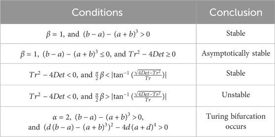
Table 1. Stability conditions of the model represented by Equation 2 at the equilibrium point $E$.

Next, by setting $a=0.5,b=0.8,\gamma =1$, the initial condition is $x_0=[a+b-0.1,b/({(a+b)}^2)-0.1]$ and the numerical solution of the model in Equation 2 is as shown in Figure 1. From Figure 1, we can see that the numerical solution of Equation 2 at the equilibrium point $E$ is asymptotically stable.

Figure 1

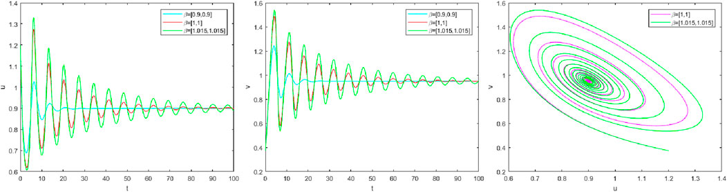
Figure 1. Numerical solution with $a=0.5,b=0.8$ and initial condition $x_0=[a+b-0.1,b/({(a+b)}^2)-0.1]$.

3 Weakly non-linear analysis

Herein, we study the dynamic behaviors of the Schnakenberg model of Equation 1 with a diffusion term at $\alpha =2$. The Jacobian matrix of Equation 2 at the equilibrium point $E$ is then given by

$J_k=\gamma \left(\begin{array}{cc}\hfill \gamma \frac{b-a}{a+b}-k^2{d}_1\hfill & \hfill {\gamma }^2{\left(a+b\right)}^2\hfill \\ \hfill -\gamma \frac{2b}{a+b}\hfill & \hfill -\gamma {\left(a+b\right)}^2-k^2{d}_2\hfill \end{array}\right).(9)$

The corresponding characteristic equation of the Schnakenberg model of Equation 1 with a diffusion term at $\alpha =2$ and equilibrium point $E$ is given by

${\lambda }^2-T{r}_k\lambda +De{t}_k=0,(10)$

where

$\begin{array}{c}T{r}_k=\gamma \frac{\left(b-a\right)-{\left(a+b\right)}^3}{a+b}-k^2\left(d_1+d_2\right),\hfill \\ De{t}_k={\gamma }^2{\left(a+b\right)}^2-\gamma \frac{d_2\left(b-a\right)-d_1{\left(a+b\right)}^3}{a+b}{k}^2+d_1{d}_2{k}^4.\hfill \end{array}(11)$

The minimum value of the perturbation $k_c$ to the system is

$k_c^2=\gamma \frac{d_2\left(b-a\right)-d_1{\left(a+b\right)}^3}{2d_1{d}_2\left(a+b\right)}.$

Thus, we obtain the eigenroot as

$\begin{array}{c}{\lambda }_{\mathrm{1,2}}=\frac{T{r}_k\pm \sqrt{T{r}_k-4De{t}_k}}{2T{r}_k}.\hfill \end{array}(12)$

The Schnakenberg model of Equation 1 experiences a Turing bifurcation when the following conditions are met:

$\begin{array}{c}\left(b-a\right)-{\left(a+b\right)}^3>0,\hfill \\ {\left(d_2\left(b-a\right)-d_1{\left(a+b\right)}^3\right)}^2>4d_2{\left(a+b\right)}^4.\hfill \end{array}(13)$

Figure 2 shows the stability and Turing instability at different values of $k$ and the diffusion coefficient. The real part of the eigenvalue greater than 0 corresponds to the Turing instability as well as stability domains.Using the methods proposed by Gao et al. as well as Chen and Zheng [34–36], we obtain the amplitude equation of the Schnakenberg model of Equation 1 at $\alpha =2$ as

$\left\{\begin{array}{cc}\hfill \frac{\varphi +\phi }{d_2^c{k}_c^2}\frac{\partial {\mathbf{A}}_1}{\partial t}& =\frac{d2-d_2^c}{d_2^c}{\mathbf{A}}_1-2\frac{h_1+\phi h_2}{d_2^c{k}_c^2}\overline{{\mathbf{A}}_2}\overline{{\mathbf{A}}_3}-\left[\frac{Q_1+\phi Q_3}{d_2^c{k}_c^2}|{\mathbf{A}}_1{|}^2+\frac{Q_2+\phi Q_4}{d_2^c{k}_c^2}\left(|{\mathbf{A}}_2{|}^2+|{\mathbf{A}}_3{|}^2\right)\right]{\mathbf{A}}_1,\hfill \\ \hfill \frac{\varphi +\phi }{d_2^c{k}_c^2}\frac{\partial {\mathbf{A}}_2}{\partial t}& =\frac{d2-d_2^c}{d_2^c}{\mathbf{A}}_2-2\frac{h_1+\phi h_2}{d_2^c{k}_c^2}\overline{{\mathbf{A}}_1}\overline{{\mathbf{A}}_3}-\left[\frac{Q_1+\phi Q_3}{d_2^c{k}_c^2}|{\mathbf{A}}_2{|}^2+\frac{Q_2+\phi Q_4}{d_2^c{k}_c^2}\left(|{\mathbf{A}}_1{|}^2+|{\mathbf{A}}_3{|}^2\right)\right]{\mathbf{A}}_2,\hfill \\ \hfill \frac{\varphi +\phi }{d_2^c{k}_c^2}\frac{\partial {\mathbf{A}}_3}{\partial t}& =\frac{d2-d_2^c}{d_2^c}{\mathbf{A}}_3-2\frac{h_1+\phi h_2}{d_2^c{k}_c^2}\overline{{\mathbf{A}}_1}\overline{{\mathbf{A}}_2}-\left[\frac{Q_1+\phi Q_3}{d_2^c{k}_c^2}|{\mathbf{A}}_3{|}^2+\frac{Q_2+\phi Q_4}{d_2^c{k}_c^2}\left(|{\mathbf{A}}_1{|}^2+|{\mathbf{A}}_2{|}^2\right)\right]{\mathbf{A}}_3,\hfill \end{array}\right.(14)$

where

$\begin{array}{c}{k}_c^2=\gamma \frac{f_u{d}_2+g_v{d}_1}{2d_1{d}_2}=\gamma \frac{d_2\left(b-a\right)-d_1{\left(a+b\right)}^3}{2d_1{d}_2\left(a+b\right)},\hfill \\ \varphi =\frac{f_v}{d_1{k}_c^2-f_u}=-\frac{2d_2{\left(a+b\right)}^3}{d_2\left(b-a\right)+d_1{\left(a+b\right)}^3},\phi =\frac{d_1{k}_c^2-f_u}{g_u}=-\frac{d_2\left(b-a\right)+d_1{\left(a+b\right)}^3}{4b{d}_2},\hfill \\ h_1=\frac{f_{uu}}{2}{\varphi }^2+f_{uv}\varphi +\frac{f_{vv}}{2}=\gamma \frac{b}{{\left(a+b\right)}^2}{\varphi }^2+2\gamma \left(a+b\right)\varphi ,h_2=\frac{g_{uu}}{2}{\varphi }^2+g_{uv}\varphi +\frac{g_{vv}}{2}=-\gamma \frac{b}{{\left(a+b\right)}^2}{\varphi }^2-2\gamma \left(a+b\right)\varphi ,\hfill \\ u_{00}=2\frac{f_v{h}_2-g_v{h}_1}{f_u{g}_v-f_v{g}_u},v_{00}=2\frac{g_u{h}_1-f_u{h}_2}{f_u{g}_v-f_v{g}_u},u_{11}=\frac{f_v{h}_2-\left(g_v-4d_2^c{k}_c^2\right)h_1}{\left(f_u-4d_1{k}_c^2\right)\left(g_v-4d_2^c{k}_c^2\right)-\left.f_v{g}_u\right)},v_{11}=\frac{g_v{h}_1-\left(f_u-4d_1{k}_c^2\right)h_2}{\left(f_u-4d_1{k}_c^2\right)\left(g_v-4d_2^c{k}_c^2\right)-\left.f_v{g}_u\right)},\hfill \\ u_{22}=2\frac{f_v{h}_2-\left(g_v-3d_2^c{k}_c^2\right)h_1}{\left(f_u-3d_1{k}_c^2\right)\left(g_v-3d_2^c{k}_c^2\right)\left.-f_v{g}_u\right)},v_{22}=2\frac{g_v{h}_1-\left(f_u-3d_1{k}_c^2\right)h_2}{\left(f_u-3d_1{k}_c^2\right)\left(g_v-4d_2^c{k}_c^2\right)-\left.f_v{g}_u\right)},\hfill \\ Q_1=\left(\varphi f_{uu}+f_{uv}\right)\left(u_{00}+u_{11}\right)+\left(\varphi f_{uv}+f_{vv}\right)\left(v_{00}+v_{11}\right)+3\gamma {\varphi }^2,\hfill \\ Q_2=\left(\varphi f_{uu}+f_{uv}\right)\left(u_{00}+u_{22}\right)+\left(\varphi f_{uv}+f_{vv}\right)\left(v_{00}+v_{22}\right)+6\gamma {\varphi }^2,\hfill \\ Q_3=\left(\varphi g_{uu}+g_{uv}\right)\left(u_{00}+u_{11}\right)+\left(\varphi g_{uv}+g_{vv}\right)\left(v_{00}+v_{11}\right)-3\gamma {\varphi }^2,\hfill \\ Q_4=\left(\varphi g_{uu}+f_{uv}\right)\left(u_{00}+u_{22}\right)+\left(\varphi g_{uv}+f_{vv}\right)\left(v_{00}+v_{22}\right)-6\gamma {\varphi }^2.\hfill \end{array}(15)$

Figure 2

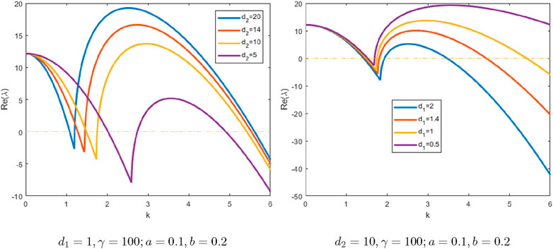
Figure 2. Stability and Turing instability curves at different perturbation values $k$.

A stable Turing spot map corresponds to a stable steady-state solution to Equation 14. Each amplitude in Equation 14 can now be decomposed into a magnitude ${\eta }_i=|{\mathbf{A}}_i|$ and a phase angle ${\mathrm{\Psi }}_i$. Substituting ${\mathbf{A}}_i={\eta }_i{e}^{i{\mathrm{\Phi }}_i}$ into Equation 14 and dividing the real and imaginary parts gives a differential equation with four real variables as follows:

$\left\{\begin{array}{cc}\hfill \frac{\varphi +\phi }{d_2^c{k}_c^2}\frac{\partial \mathrm{\Psi }}{\partial t}& =2\frac{h_1+\phi h_2}{d_2^c{k}_c^2}\frac{{\eta }_1^2{\eta }_2^2+{\eta }_1^2{\eta }_3^2+{\eta }_2^2{\eta }_3^2}{{\eta }_1{\eta }_2{\eta }_3}\sin \mathrm{\Psi },\hfill \\ \hfill \frac{\varphi +\phi }{d_2^c{k}_c^2}\frac{\partial {\eta }_1}{\partial t}& =\frac{d2-d_2^c}{d_2^c}{\eta }_1-2\frac{h_1+\phi h_2}{d_2^c{k}_c^2}{\eta }_2{\eta }_3\cos \mathrm{\Psi }-\frac{Q_1+\phi Q_3}{d_2^c{k}_c^2}{\eta }_1^3-\frac{Q_2+\phi Q_4}{d_2^c{k}_c^2}\left({\eta }_2^2+{\eta }_3^2\right){\eta }_1,\hfill \\ \hfill \frac{\varphi +\phi }{d_2^c{k}_c^2}\frac{\partial {\eta }_2}{\partial t}& =\frac{d2-d_2^c}{d_2^c}{\eta }_2-2\frac{h_1+\phi h_2}{d_2^c{k}_c^2}{\eta }_1{\eta }_3\cos \mathrm{\Psi }-\frac{Q_1+\phi Q_3}{d_2^c{k}_c^2}{\eta }_2^3-\frac{Q_2+\phi Q_4}{d_2^c{k}_c^2}\left({\eta }_1^2+{\eta }_3^2\right){\eta }_2,\hfill \\ \hfill \frac{\varphi +\phi }{d_2^c{k}_c^2}\frac{\partial {\eta }_3}{\partial t}& =\frac{d2-d_2^c}{d_2^c}{\eta }_3-2\frac{h_1+\phi h_2}{d_2^c{k}_c^2}{\eta }_1{\eta }_2\cos \mathrm{\Psi }-\frac{Q_1+\phi Q_3}{d_2^c{k}_c^2}{\eta }_3^3-\frac{Q_2+\phi Q_4}{d_2^c{k}_c^2}\left({\eta }_1^2+{\eta }_2^2\right){\eta }_3,\hfill \end{array}\right.(16)$

where $\mathrm{\Psi }={\mathrm{\Psi }}_1+{\mathrm{\Psi }}_2+{\mathrm{\Psi }}_3$. Equation 16 shows that when the system is in the steady state, the amplitude phase diagram of the combined phase can assume only two steady states as $\mathrm{\Psi }=0$ and $\mathrm{\Psi }=\pi$. If we consider only the stable solution of Equation 16, then the magnitude equation has the form

$\left\{\begin{array}{cc}\hfill \frac{\varphi +\phi }{d_2^c{k}_c^2}\frac{\partial {\eta }_1}{\partial t}& =\mu {\eta }_1+|h|{\eta }_2{\eta }_3-g_1{\eta }_1^3-g_2\left({\eta }_2^2+{\eta }_3^2\right){\eta }_1,\hfill \\ \hfill \frac{\varphi +\phi }{d_2^c{k}_c^2}\frac{\partial {\eta }_2}{\partial t}& =\mu {\eta }_2+|h|{\eta }_1{\eta }_3-g_1{\eta }_2^3-g_2\left({\eta }_1^2+{\eta }_3^2\right){\eta }_2,\hfill \\ \hfill \frac{\varphi +\phi }{d_2^c{k}_c^2}\frac{\partial {\eta }_3}{\partial t}& =\mu {\eta }_3+|h|{\eta }_1{\eta }_2-g_1{\eta }_3^3-g_2\left({\eta }_1^2+{\eta }_2^2\right){\eta }_3,\hfill \end{array}\right.(17)$

where

$\begin{array}{c}\hfill \mu =\frac{d2-d_2^c}{d_2^c},h=-2\frac{h_1+\phi h_2}{d_2^c{k}_c^2},{\tau }_0=\frac{\varphi +\phi }{d_2^c{k}_c^2},g_1=\frac{Q_1+\phi Q_3}{d_2^c{k}_c^2},g_2=\frac{Q_2+\phi Q_4}{d_2^c{k}_c^2}.\end{array}(18)$

Since the second-order coefficients $|h|$ are always positive and destabilizing factors of the equation, the third-order terms $g_1,g_2$must be positive to maintain the steady-state solution of the mode equation. Thus, Equation 17 has four classes of steady-state solutions, as shown in Table 2.

Table 2

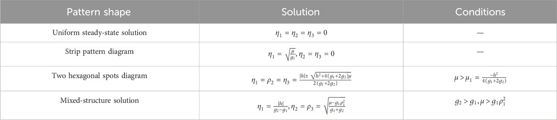
Table 2. Relationships between pattern shapes and steady-state solutions.

For $\frac{g_2}{g_1}<1$, the fringe pattern will be unstable. In Equation 17, to obtain the steady-state solution of $(\delta {\eta }_1,\delta {\eta }_2,\delta {\eta }_3)$ with perturbation, the original equation is applied and high-order items are removed to derive the linear perturbation equation. Thus, the matrix form of the equation is given as

$\begin{array}{c}(\mu -3g_1{\eta }_1^2-g_2\left({\eta }_2^2+{\eta }_3^2\right)|h|{\eta }_3-2g_2{\eta }_1{\eta }_2|h|{\eta }_2-2g_2{\eta }_1{\eta }_3\\ |h|{\rho }_3-2g_2{\eta }_1{\eta }_2\mu -3g_1{\eta }_2^2-g_2\left({\eta }_1^2+{\eta }_3^2\right)|h|{\eta }_1-2g_2{\eta }_2{\eta }_3|h|{\eta }_2-2g_2{\eta }_1{\eta }_3|h|{\eta }_1-2g_2{\eta }_2{\eta }_3\mu -3g_1{\eta }_3^2-g_2\left({\eta }_1^2+{\eta }_2^2\right))\end{array}.(19)$

The linear stability of the bar pattern is studied next. By substituting the steady-state solution $(\rho ,\mathrm{0,0})$ into the perturbation expression of Equation 19, we get

${\tau }_0\frac{d}{dt}\left(\begin{array}{c}\hfill \delta {\eta }_1\hfill \\ \hfill \delta {\eta }_2\hfill \\ \hfill \delta {\eta }_3\hfill \end{array}\right)=\left(\begin{array}{ccc}\hfill \mu -3g_1{\eta }^2\hfill & \hfill 0\hfill & \hfill 0\hfill \\ \hfill 0\hfill & \hfill \mu -g_2{\eta }^2\hfill & \hfill |h|\eta \hfill \\ \hfill 0\hfill & \hfill |h|\eta \hfill & \hfill \mu -g_2{\eta }^2\hfill \end{array}\right)\left(\begin{array}{c}\hfill \delta {\eta }_1\hfill \\ \hfill \delta {\eta }_2\hfill \\ \hfill \delta {\eta }_3\hfill \end{array}\right).(20)$

Because $\eta =\sqrt{\frac{\mu }{g_1}}$, the corresponding matrix eigenvalue $s_i$ of Equation 20 is obtained using the following characteristic equation:

$\left(-2\mu -s\right)\left({\left(\mu -\frac{g_2}{g_1}-s\right)}^2-\frac{|h{|}^2}{g_1}\mu \right)=0.(21)$

The three eigenvalues are then obtained as

$s_1=-2\mu ,s_2=s_3=\mu \left(1-\frac{g_2}{g_1}\right)\pm |h|\sqrt{\frac{\mu }{g_1}}.(22)$

Since $\mu >0,\frac{g_2}{g_1}>1$, the condition for which all three eigenvalues are simultaneously less than 0 is $\mu >{\mu }_3=\frac{h^2{g}_1}{{(g_1-g_2)}^2}$. Under this condition, the perturbation of the stripe pattern will disappear with time.

4 Brief description of the numerical algorithm

The Fourier spectral method is a numerical approach for solving partial differential equations based on the Fourier series expansion and Fourier transform. In this work, we apply the fast Fourier transform to the Schnakenberg model of Equation 1 to obtain the following ordinary differential equations:

$\left\{\begin{array}{c}\frac{d\tilde{u}}{dt}=|\kappa {|}^{\alpha }\tilde{u}+\gamma \left(a-\tilde{u}+\mathbb{F}\left(u^{2}v\right)\right),\hfill \\ \frac{d\tilde{v}}{dt}=d|\kappa {|}^{\alpha }\tilde{v}+\gamma \left(b-\mathbb{F}\left(u^{2}v\right)\right),\hfill \\ \tilde{u}\left(\kappa ,0\right)={\tilde{u}}_0\left(\kappa \right),\tilde{v}\left(\kappa ,0\right)={\tilde{v}}_0\left(\kappa \right),\kappa \in R.\hfill \end{array}\right.(23)$

Then, the fourth-order Runge–Kutta method is used to solve the ordinary differential equations in Equation 23. This can greatly simplify the calculations and help solve the Schnakenberg model of Equation 1 effectively.

5 Numerical simulation

In the numerical simulations, the spatial domain is given by $(x,y)\in [-\mathrm{2,2}]\times [-\mathrm{2,2}]$, and the spatial step size is $h=4/256$ with a time step of 0.01. In this work, we only show the pattern for $u$.

Experiment 1 Consider the following Schnakenberg model:

$\left\{\begin{array}{c}\frac{\partial 1}{\partial t}=d_u{\nabla }^{\alpha }u+\gamma \left(a-u+u^{2}v\right),\hfill \\ \frac{\partial 2}{\partial t}=d_v{\nabla }^{\alpha }v+\gamma \left(b-u^{2}v\right),\hfill \end{array}\right.(24)$

with the following initial conditions [37]:

$\left\{\begin{array}{cc}\hfill u\left(x,y,0\right)& =a+b+10^{-3}{\exp }^{-100\left[{\left(x-\frac{1}{3}\right)}^2+{\left(y-\frac{1}{2}\right)}^2\right]},\hfill \\ \hfill v\left(x,y,0\right)& =\frac{b}{{\left(a+b\right)}^2}.\hfill \end{array}\right.(25)$

We set the parameters as $d_1=0.05,d_2=1,\gamma =100,a=0.1305,b=0.7695$, and the equilibrium point is $(u_o,v_o)=(0.9,0.95)$. Next, we observe different pattern dynamic behaviors by setting the perturbation and initial conditions as shown in Table 3. The corresponding numerical simulation results are shown in Figures 3–5.

Table 3

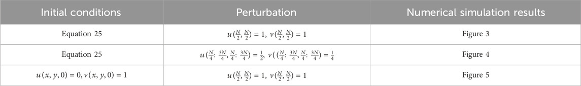
Table 3. Condition selection and numerical simulation results.

Figure 3

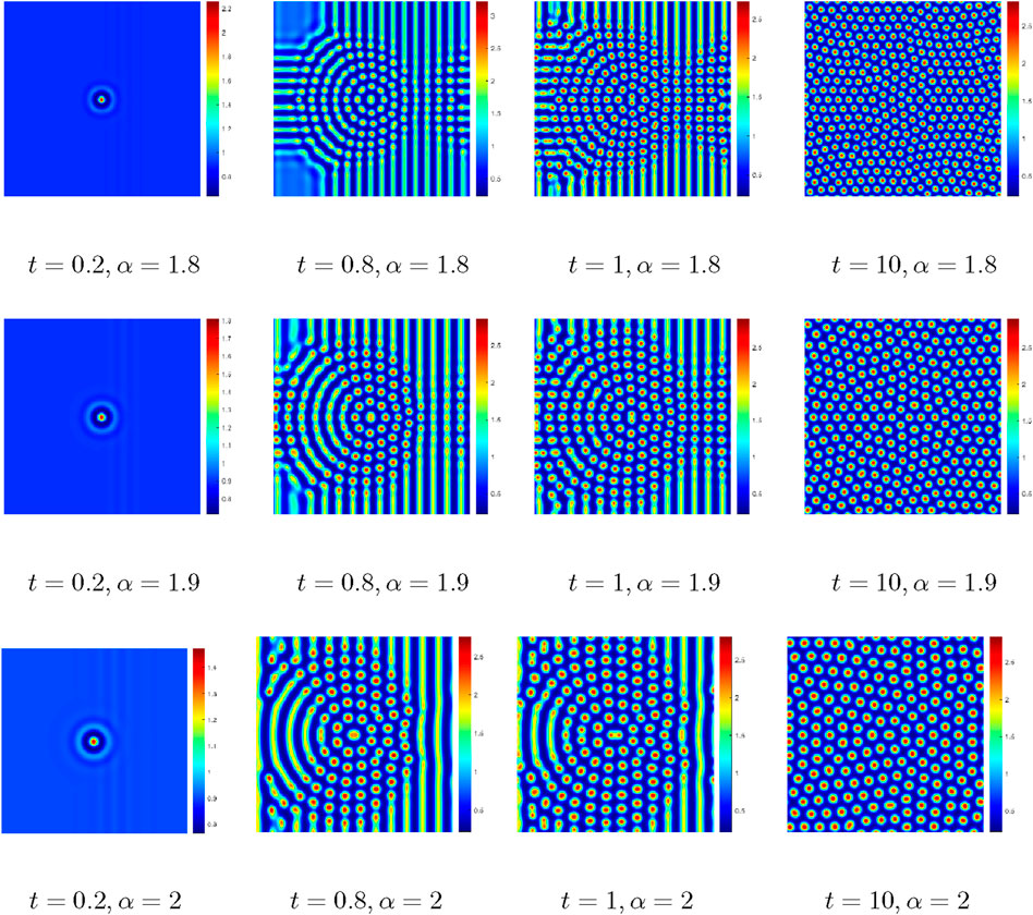
Figure 3. Comparison of the numerical results at different fractional orders with $d_1=0.05,d_2=1,\gamma =100,a=0.1305$, $b=0.7695$ and the initial conditions in Equation 25 for Experiment 1.

Figure 4

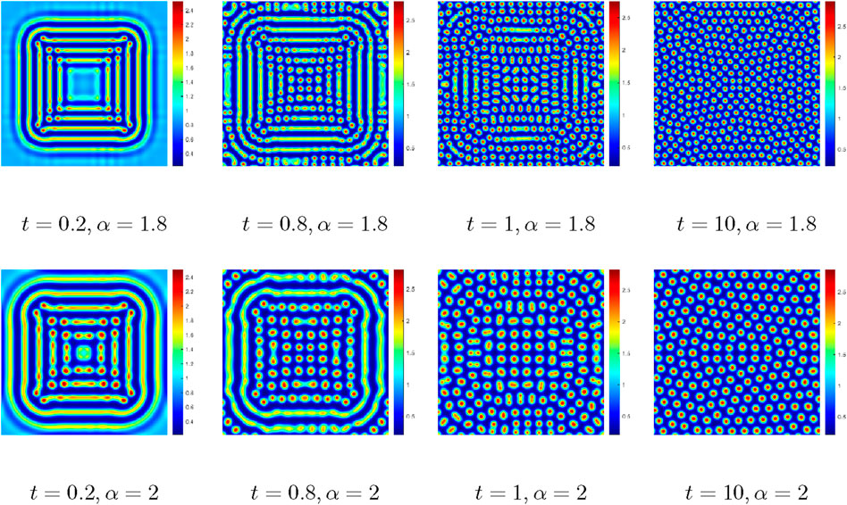
Figure 4. Comparison of the numerical results at different fractional orders with perturbations $u(\frac{N}{4}:\frac{3N}{4},\frac{N}{4}:\frac{3N}{4})=\frac{1}{2}$, $v(\frac{N}{4}:\frac{3N}{4},\frac{N}{4}:\frac{3N}{4})=\frac{1}{4}$ for Experiment 1.

Figure 5

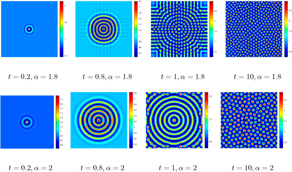
Figure 5. Comparison of the numerical results at different fractional orders with initial conditions of $u(x,y,0)=0,v(x,y,0)=1$ for Experiment 1.

Figure 3 shows different Turing patterns by setting the value of $\alpha$ over a certain period of time. We observe from the pattern that as time elapses, the reaction substance diffuses in this region, and the more the reaction order is closer to an integer value, the slower is the diffusion rate. We also observe that the fractional pattern is composed of several irregular polygons. The figure shows that when $\alpha$ is reduced, this pattern is dynamic; when $\alpha$ is closer to 1, the pattern splits faster, which is an overdiffusion process. We thus retain the parameters and initial conditions unchanged while changing the perturbation to $u(\frac{N}{4}:\frac{3N}{4},\frac{N}{4}:\frac{3N}{4})=\frac{1}{2},v(\frac{N}{4}:\frac{3N}{4},\frac{N}{4}:\frac{3N}{4})=\frac{1}{4}$, for which the pattern dynamic behaviors of the fractional-in-space Schnakenberg model are shown in Figure 4.

From Figure 4, it is observed that the perturbation has a huge impact on the spot pattern. Figures 3, 4 have the same parameters and initial conditions, and changing the perturbation results in a large difference between the initial state and final spot pattern. However, these two figures have almost similar diffusion rates; thus, as $\alpha$ decreases, the diffusion is more intense and the small ring is more crowded.Next, after setting the different parameters and adjusting the initial conditions as $u(x,y,0)=0,v(x,y,0)=1$ and $u(\frac{N}{2},\frac{N}{2})=1$, the target model produces the results shown in Figure 5. Figure 5 is a typical target-type pattern that is also symmetrical during diffusion. This pattern consists of small to large rings, which expand gradually with time and then break into smaller rings.

From Figures 3–5, we note that the formation of the pattern of the Schnakenberg model of Eq. Equation 24 depends on the selected parameters. Only those parameters that meet certain conditions produce the Turing pattern, and the fractional order affects the diffusion speed of this pattern. Variations in the initial conditions and perturbations will lead to differences in the pattern. The present numerical simulation results are in good agreement with the conclusions reported by Arafa et al. [37] using homotopy analysis for the fractional-order Schnakenberg model.

Experiment 2 Consider the Schnakenberg model of Equation 24 with periodic boundary conditions [38] as follows:

$\left\{\begin{array}{cc}\hfill u\left(x,y,0\right)& =0.919145+0.0016\cos \left(2\pi \left(x+y\right)\right)+0.01{\displaystyle \sum _{j=1}^8}\cos \left(2\pi jx\right),\hfill \\ \hfill v\left(x,y,0\right)& =0.937903+0.0016\cos \left(2\pi \left(x+y\right)\right)+0.01{\displaystyle \sum _{j=1}^8}\cos \left(2\pi jx\right).\hfill \end{array}\right.(26)$

By setting the parameters as $d_u=1,d_v=10,\gamma =1000,a=0.126779,b=0.792366$, and $\mathrm{\Omega }=[\mathrm{0,1}]\times [\mathrm{0,1}]$, we simulated a Turing pattern with periodic boundary conditions [38] and different initial conditions. The numerical simulation results for Equation 24 using the Fourier spectral method are shown in Figures 6–8. Furthermore, Table 4 shows the corresponding spot patterns for different fractional orders.By setting $\alpha =1.9$ and the perturbations to $u(\frac{N}{2},\frac{N}{2})=1,v(\frac{N}{2},\frac{N}{2})=1$ in Equation 26, we observe the distortion instability of the bar pattern in Figure 6. Once the distortion instability occurs, the local wavelength of the system gradually reduces, and the amplitude of the modulated wave will saturate under the action of the higher-order terms. The warped instability results in a new symmetry breakdown, producing a warped bar pattern as shown in Figure 6, which has a lower symmetry than the original pattern. Next, by maintaining the parameters and initial conditions unchanged in Equation 26, we obtain the numerical simulation results under different fractional orders, and the corresponding pattern dynamic behaviors of the fractional-in-space Schnakenberg model are shown in Figure 7.In Figure 7, when $\alpha =1.7,1.6$, it is observed from the graphs that the spot chart that is initially in the form of pipes changes so that each pipe splits into small circles. An ordered arrangement is formed, and as the value of $\alpha$ decreases, the small rings in the pipe change from two to three columns while the speed of splitting also decreases. From Figures 6, 7, we can confirm that the initial conditions of the strip produce a spot pattern after a series of diffusions. This is consistent with the conclusions noted by Vivek et al. [38] using a new implicit-explicit Runge–Kutta method to calculate the Schnakenberg model of Equation 1. Next, we maintain the parameters unchanged while altering the initial conditions to $u(x,y,0)=0,v(x,y,0)=1$ and perturbations to $v(\frac{N}{2},\frac{N}{2})=1$; these simulation results are shown in Figure 7. It is seen from Figure 8 that when $\alpha$ decreases, the Turing pattern spreads more violently and is arranged more neatly.

Figure 6

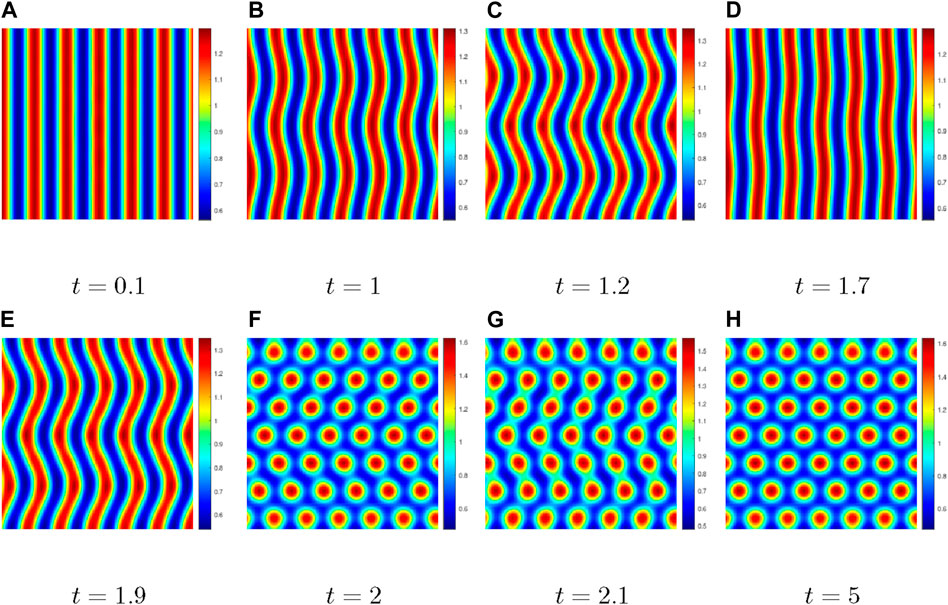
Figure 6. Comparison of the numerical results with $d_1=1,d_2=10,\gamma =1000$, $a=0.126779,b=0.792366$, $\alpha =1.9$, and the initial conditions in Equation 26 for Experiment 2.

Figure 7

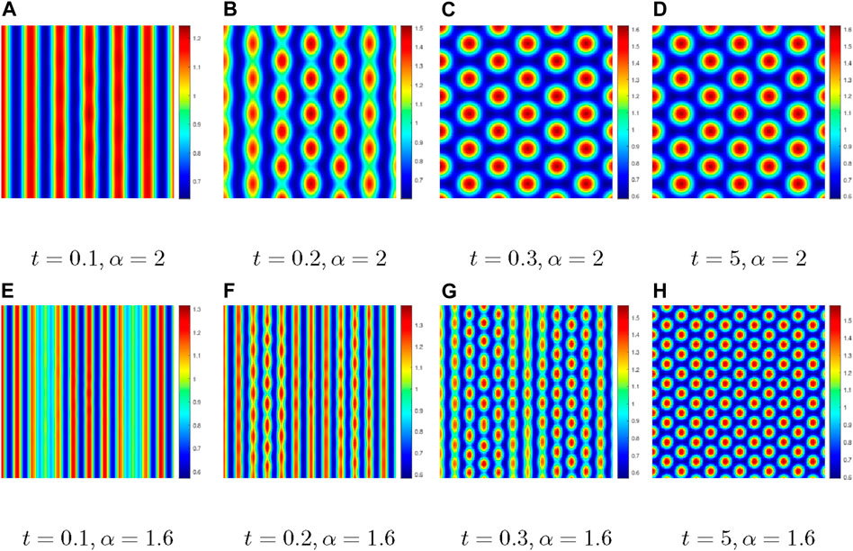
Figure 7. Comparison of the pattern dynamic behaviors with $d_1=1,d_2=10,\gamma =1000$, $a=0.126779,b=0.792366$, $\alpha =1.9$, and the initial conditions in Equation 26 for Experiment 2.

Figure 8

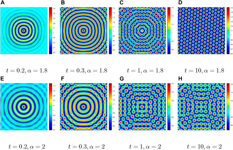
Figure 8. Comparison of the pattern dynamic behaviors at different fractional orders with $d_1=1,d_2=10,\gamma =1000$, $a=0.126779,b=0.792366$ and initial conditions of $u(x,y,0)=0,v(x,y,0)=1$ for Experiment 2.

Table 4

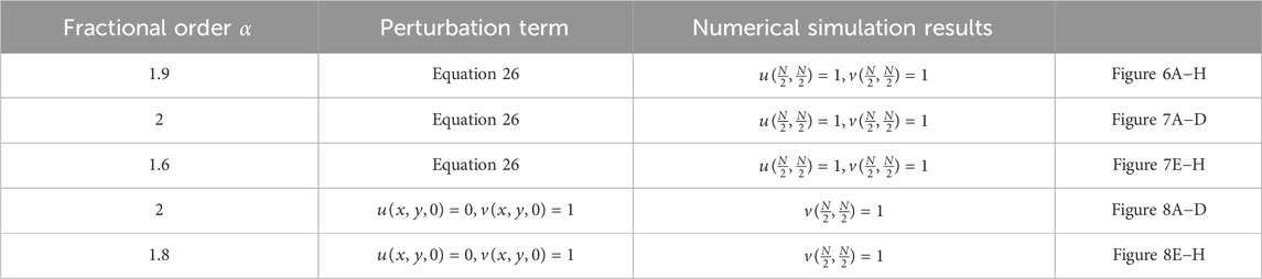
Table 4. Fractional-order selection and numerical simulation results.

6 Conclusion

In this work, the Fourier spectral method was used to study the pattern dynamic behaviors of the fractional-in-space Schnakenberg model using multiple sets of parameters, initial conditions, perturbations, and fractional orders. After counting, different types of patterns were obtained, including the target, dot, and strip patterns. During the numerical simulations, we observed that the patterns not only diffused from a single point to a dense spot pattern but also split from the bar pattern into a spot pattern; further, it was observed that the point pattern could also merge into a bar pattern. We noted that the Turing model was very sensitive to the parameters and that the influences of the initial conditions on pattern formation cannot be ignored. The numerical results are in good agreement with findings based on other methods reported in literature. Some novel patterns were also observed in this work. The theoretical analysis and numerical simulation results of the fractional-in-space Schnakenberg model presented herein contribute to a broader understanding of the formation and dynamic behaviors of the Schnakenberg pattern. The roles of fractional operators in promoting diffusion are also better understood. In the future, we intend to develop hybrid methods by combining the Fourier spectral method with other numerical techniques to study some fractional-order partial differential equations [39, 40].

Data availability statement

The original contributions presented in the study are included in the article/Supplementary Material, and any further inquiries may be directed to the corresponding authors.

Author contributions

J-LW: conceptualization and writing–original draft. Y-XH: software and writing–review and editing. Q-TC: data curation, methodology, and writing–review and editing. Z-YL: formal analysis, funding acquisition, and writing–review and editing. M-JD: funding acquisition, and writing–original draft. Y-LW: data curation, resources, and writing–review and editing.

Funding

The authors declare that financial support was received for the research, authorship, and/or publication of this article. This work was supported by the Talent Development Foundation of Inner Mongolia Autonomous Region (to Ming-Jing Du), University Basic Research Funds Project of Inner Mongolia Autonomous Region (no. NCYWT23023), High-Quality Research Achievements Cultivation Fund of Inner Mongolia University of Finance and Economics (no. GZCG2487), Doctoral Research Startup Fund of Inner Mongolia University of Technology (nos. DC2300001252 and DC2200000935), and Natural Science Foundation of Inner Mongolia (no. 2024LHMS06025).

Conflict of interest

The authors declare that the research was conducted in the absence of any commercial or financial relationships that could be construed as a potential conflict of interest.

Publisher’s note

All claims expressed in this article are solely those of the authors and do not necessarily represent those of their affiliated organizations or those of the publisher, editors, and reviewers. Any product that may be evaluated in this article or claim that may be made by its manufacturer is not guaranteed or endorsed by the publisher.

References

1. Li CP, Wang Z. Numerical methods for the time fractional convection-diffusion-reaction equation. Numer Funct Anal Optimization (2021) 42(10):1115–53. doi:10.1080/01630563.2021.1936019

CrossRef Full Text | Google Scholar

2. He JH, He CH, Qian MY, Alsolami AA. Piezoelectric Biosensor based on ultrasensitive MEMS system. Sensors Actuators A: Phys (2024) 376:115664. doi:10.1016/j.sna.2024.115664

CrossRef Full Text | Google Scholar

3. He JH, Yang Q, He CH, Alsolami AA. Pull-down instability of the quadratic nonlinear oscillator, Facta Universitatis, Series. Mech Eng (2023) 21(2):191–200. doi:10.22190/fume230114007h

CrossRef Full Text | Google Scholar

4. Gao XL, Li ZY, Wang YL. Chaotic dynamic behavior of a fractional-order financial system with constant inelastic demand. Int J Bifurcation Chaos (2024) 34(9):2450111. doi:10.1142/s0218127424501116

CrossRef Full Text | Google Scholar

5. He JH, Jiao ML, He CH. Homotopy perturbation method for fractal duffing oscillators with arbitrary conditions. Fractals (2022) 30(9):2250165. doi:10.1142/s0218348x22501651

CrossRef Full Text | Google Scholar

6. Li ZY, Chen QT, Wang YL, Li XY. Solving two-sided fractional super-diffusive partial differential equations with variable coefficients in a class of new reproducing kernel spaces. Fractal and Fractional (2022) 6(9):492. doi:10.3390/fractalfract6090492

CrossRef Full Text | Google Scholar

7. Onarcan AT, Adar N, Dag I. Pattern formation of Schnakenberg model using trigonometric quadratic B-spline functions. Pramana-Journal Phys (2022) 96(3):138. doi:10.1007/s12043-022-02367-2

CrossRef Full Text | Google Scholar

8. Khan FM, Ali A, Hamadneh N, Abdullah AMN. Numerical investigation of chemical Schnakenberg mathematical Model. J Nanomater (2021) 2021:1–8. doi:10.1155/2021/9152972

CrossRef Full Text | Google Scholar

9. Fragnelli G, Mugnai D. Turing patterns for a coupled two-cell generalized Schnakenberg model. Complex Variables and Elliptic Equations (2020) 65(8):1343–59. doi:10.1080/17476933.2019.1631291

CrossRef Full Text | Google Scholar

10. Din Q, Haider K. Discretization, bifurcation analysis and chaos control for Schnakenberg model. J Math Chem (2020) 58(8):1615–49. doi:10.1007/s10910-020-01154-x

CrossRef Full Text | Google Scholar

11. Al Noufaey KS. Stability analysis for Selkov-Schnakenberg reaction-diffusion system. Open Mathematics (2021) 19(1):46–62. doi:10.1515/math-2021-0008

CrossRef Full Text | Google Scholar

12. Yang R. Turing-Hopf bifurcation co-induced by cross-diffusion and delay in Schnakenberg system. Chaos, Solitons & Fractals (2022) 164:112659. doi:10.1016/j.chaos.2022.112659

CrossRef Full Text | Google Scholar

13. Al Noufaey KS. A semi-analytical approach for the reversible Schnakenberg reaction-diffusion system. Results Phys (2020) 16:102858. doi:10.1016/j.rinp.2019.102858

CrossRef Full Text | Google Scholar

14. Yang R. Cross-diffusion induced spatiotemporal patterns in Schnakenberg reaction-diffusion model. Nonlinear Dyn (2022) 110(2):1753–66. doi:10.1007/s11071-022-07691-1

CrossRef Full Text | Google Scholar

15. Liu Y, Wei X. Turing-Hopf bifurcation analysis of the Sel’kov-Schnakenberg system. Int J Bifurcation Chaos (2023) 33(01):2350012. doi:10.1142/s0218127423500128

CrossRef Full Text | Google Scholar

16. Xu Y, Ren J, Li X, Zhu D. On the Schnakenberg model with crucial reversible reactions. Math Methods Appl Sci (2024) 47(4):2452–71. doi:10.1002/mma.9757

CrossRef Full Text | Google Scholar

17. Zhang H, Jiang X, Wang C, Chen S. Crank-Nicolson Fourier spectral methods for the space fractional nonlinear Schrödinger equation and its parameter estimation. Int J Computer Mathematics (2019) 96(2):238–63. doi:10.1080/00207160.2018.1434515

CrossRef Full Text | Google Scholar

18. Zou G, Wang B, Sheu TWH. On a conservative Fourier spectral Galerkin method for cubic nonlinear Schrödinger equation with fractional Laplacian. Mathematics Comput Simulation (2020) 168:122–34. doi:10.1016/j.matcom.2019.08.006

CrossRef Full Text | Google Scholar

19. Harris AP, Biala TA, Khaliq AQM. Fourier spectral methods with exponential time differencing for space-fractional partial differential equations in population dynamics. Numer Methods Partial Differential Equations (2023) 39(4):2963–74. doi:10.1002/num.22995

CrossRef Full Text | Google Scholar

20. Lee HG. A second-order operator splitting Fourier spectral method for fractional-in-space reaction-diffusion equations. J Comput Appl Mathematics (2018) 333:395–403. doi:10.1016/j.cam.2017.09.007

CrossRef Full Text | Google Scholar

21. Chen L, Lu S. Fourier spectral approximation for generalized time fractional Burgers equation. J Appl Mathematics Comput (2022) 68(6):3979–97. doi:10.1007/s12190-021-01686-8

CrossRef Full Text | Google Scholar

22. Arezoomandan M, Soheili AR. Spectral collocation method for stochastic partial differential equations with fractional Brownian motion. J Comput Appl Mathematics (2021) 389:113369. doi:10.1016/j.cam.2020.113369

CrossRef Full Text | Google Scholar

23. Qu H, She Z. Fourier spectral method with an adaptive time strategy for nonlinear fractional Schrodinger equation. Numer Methods Partial Differential Equations (2020) 36(4):823–38. doi:10.1002/num.22453

CrossRef Full Text | Google Scholar

24. Weng Z, Zhai S, Feng X. A Fourier spectral method for fractional-in-space Cahn-Hilliard equation. Appl Math Model (2017) 42:462–77. doi:10.1016/j.apm.2016.10.035

CrossRef Full Text | Google Scholar

25. Pindza E, Owolabi KM. Fourier spectral method for higher order space fractional reaction-diffusion equations. Commun Nonlinear Sci Numer Simulation (2016) 40:112–28. doi:10.1016/j.cnsns.2016.04.020

CrossRef Full Text | Google Scholar

26. Fakhar-Izadi F, Shabgard N. Time-space spectral Galerkin method for time-fractional fourth-order partial differential equations. J Appl Mathematics Comput (2022) 68(6):4253–72. doi:10.1007/s12190-022-01707-0

CrossRef Full Text | Google Scholar

27. Che H, Yu-Lan W, Zhi-Yuan L. Novel patterns in a class of fractional reaction-diffusion models with the Riesz fractional derivative. Mathematics Comput Simulation (2022) 202:149–63. doi:10.1016/j.matcom.2022.05.037

CrossRef Full Text | Google Scholar

28. Han C, Wang YL, Li ZY. A high-precision numerical approach to solving space fractional Gray-Scott model. Appl Mathematics Lett (2022) 125:107759. doi:10.1016/j.aml.2021.107759

CrossRef Full Text | Google Scholar

29. Kong XX, Yu F, Yao W, Cai S, Zhang J, Lin HR. Memristor-induced hyperchaos, multiscroll and extreme multistability in fractional-order HNN: image encryption and FPGA implementation. Neural Networks (2024) 171:85–103. doi:10.1016/j.neunet.2023.12.008

PubMed Abstract | CrossRef Full Text | Google Scholar

30. Wei JL, Wu GC, Liu BQ, Zhao ZG. New semi-analytical solutions of the time-fractional Fokker-Planck equation by the neural network method. Optik (2022) 259:168896. doi:10.1016/j.ijleo.2022.168896

CrossRef Full Text | Google Scholar

31. Wu GC, Wei JL, Xia TC. Multi-layer neural networks for data-driven learning of fractional difference equations’ stability, periodicity and chaos. Physica D: Nonlinear Phenomena (2024) 457:133980. doi:10.1016/j.physd.2023.133980

CrossRef Full Text | Google Scholar

32. Zhang LH, Liu Q, Ahmad B, Wang GT. Nonnegative solutions of a coupled k-Hessian system involving different fractional Laplacians. Fractional Calculus and Applied Analysis (2024) 27(4):1835–1851. doi:10.1007/s13540-024-00277-1

CrossRef Full Text | Google Scholar

33. Yu F, Zhang W, Xiao X, Yao W, Cai S, Zhang J, et al. Dynamic analysis and field-programmable gate array implementation of a 5D fractional-order memristive hyperchaotic system with multiple coexisting attractors. Fractal and Fractional (2024) 8(5):271. doi:10.3390/fractalfract8050271

CrossRef Full Text | Google Scholar

34. Gao XL, Zhang HL, Li XY. Research on pattern dynamics of a class of predator-prey model with interval biological coefficients for capture. AIMS Mathematics (2024) 9(7):18506–27. doi:10.3934/math.2024901

CrossRef Full Text | Google Scholar

35. Gao XL, Zhang HL, Wang YL, Li ZY. Research on pattern dynamics behavior of a fractional vegetation-water model in arid flat environment. Fractal and Fractional (2024) 8(5):264. doi:10.3390/fractalfract8050264

CrossRef Full Text | Google Scholar

36. Chen MX, Zheng QQ. Diffusion-driven instability of a predator-prey model with interval biological coefficients. Chaos, Solitons and Fractals (2023) 172:113494. doi:10.1016/j.chaos.2023.113494

CrossRef Full Text | Google Scholar

37. Arafa AAM, Rida SZ, Mohamed H. Approximate analytical solutions of Schnakenberg systems by homotopy analysis method. Appl Math Model (2012) 36(10):4789–96. doi:10.1016/j.apm.2011.12.014

CrossRef Full Text | Google Scholar

38. Vivek SY, Vikas M, Manoj KR, Jyoti J. Spatiotemporal pattern formations in stiff reaction-diffusion systems by new time marching methods. Appl Mathematics Comput (2022) 431:127299. doi:10.1016/j.amc.2022.127299

CrossRef Full Text | Google Scholar

39. Zhang RF, Li MC, Cherraf A, Vadyala SR. The interference wave and the bright and dark soliton for two integro-differential equation by using BNNM. Nonlinear Dyn (2023) 111(9):8637–46. doi:10.1007/s11071-023-08257-5

CrossRef Full Text | Google Scholar

40. Zhang RF, Bilige S. Bilinear neural network method to obtain the exact analytical solutions of nonlinear partial differential equations and its application to p-gBKP equatuon. Nonlinear Dyn (2019) 95:3041–8. doi:10.1007/s11071-018-04739-z

CrossRef Full Text | Google Scholar