HMAE: a high-fidelity multi-agent simulator for economic phenomenon emergence

Economic models based on multi-agents are increasingly attracting attention and can provide a new perspective for exploring the causes behind social phenomena at the individual level. Existing research usually adopts society-level learning methods, and more research on micro-level heterogeneity among individuals is needed. For this, we propose a high-fidelity multi-agent economy (HMAE) model based on evolutionary game theory, including three types of agents: workers, firms, and the government. In particular, we characterize worker heterogeneity regarding laziness factors, work endowments, and commuting distances. These agents continuously and iteratively update their strategies by randomly exploring and imitating their neighbors to maximize their utility value. We simulated the evolution process of agent behavioral decisions through experiments and found that individual heterogeneity can significantly affect the decisions of workers and firms. These phenomena are consistent with some economic evolution trends in real life, and our research can provide an analytical tool for analyzing the causes of emerging economic phenomena.

1 Introduction

The economy is an evolving, complex, and dynamic system in which the interaction of micro-agents produces global regularities, such as employment and growth rates, income distribution, market institutions, and social customs [1–6]. The unpredictability of economic systems has attracted the interest of many researchers, who focus on building simple and reasonable economic models to analyze the reasons behind behaviors by simulating real-world phenomena [7–9]. Understanding and predicting human group behavior requires an understanding and reasoning about complex economic systems.

Over the past two centuries, there has been a fundamental change in the way economic science is studied; it has become a social science based on mathematical models rather than words [10]. Traditional economic models, i.e., econometric models and dynamic stochastic general equilibrium (DSGE) models [11–13], have been widely developed in “normal times” like the Great Moderation Period [14]. Typical econometric models, such as vector autoregressive (VAR) models [15–17] and structure VAR models [18–20], have gained increasing popularity, especially in empirical macroeconomics. Subsequently, DSGE models such as the Chameleon model [21] and the New Keynesian (NK) DSGE model [22, 23] were developed to bridge the gap between the structural characteristics of the economy and simplified parameterization [24]. The DSGE model regards the macroeconomic model as a representative agent behavior that is consistent with microeconomic theory and aims to explain macroeconomic behavior. However, traditional economic models cannot predict the outbreak of economic crises and analyze the influencing factors behind the phenomenon, mainly for two reasons. First, these models are based on simplified assumptions and a lack of characterization at the micro level. In addition, due to the complexity of the real economy and limitations of computing power [25–27], the model only uses aggregate data such as the gross domestic product (GDP) and unemployment rate, resulting in vast amounts of data that cannot be used to gain a deeper understanding of economic performance [28]. Second, when analyzing new economic phenomena, a large amount of historical data is needed to evaluate parameters, which brings difficulties to the generalization and portability of the model [29, 30].

With the emergence and development of computer simulation technology, an agent-based model (ABM) that builds artificial social systems “from the bottom up” has received more attention and been applied in economic studies [6, 31–33]. The advantage of the ABM is that it allows economists to validate hypotheses [34] at the individual levels and in which the relationships among several heterogeneous objects generate regularities that can change over time. This bottom-up research method makes up for the shortcomings of traditional macroeconomic models in studying microscopic phenomena and shows superior capabilities [35, 36]. [37], [38], and [39] presented the application of the ABM in different research areas and explored the types of scenarios that the ABM can reproduce. [40] used the ABM to study the effect of different labor market integration policies on economic performance and convergence of two distinct regions. [41] investigated the economic impact of feed-in tariff policy mechanisms designed to promote investment in renewable energy capacity based on ABM methods. Utilizing the representational strength of neural networks, [42–44] aimed to create agents that can follow instructions for manipulation, navigation, or both. [45] introduced a social norm ABM that promotes division of labor by redistributing rewards. However, current research usually conducts society-level learning or adopts methods that incorporate more advanced optimization concepts into the ABM [46], lacking individual-level learning, which means a lack of heterogeneity among individuals [31, 47–49]. For example, individuals are only classified as high-skilled and low-skilled, lacking a finer description of multiple characteristics at the micro-level.

To make up for the shortcomings of the above research and design a simulator that can connect the relationships between heterogeneous individuals to spread information and resources, we propose a high-fidelity multi-agent economic model. Specifically, this paper aims to design a model that can more realistically describe real-world economic activities, help analysts simulate significant economic behaviors, and analyze the reasons behind some real-world economic phenomena to provide better suggestions for future economic policy formulation. The main contributions of our work are outlined as follows:

$•$ We propose a high-fidelity multi-agent economy (HMAE) model to study the evolution of interactions between agents, focusing on the heterogeneity of individuals at the micro-level and the impact of external factors on agent decision-making. This model describes the heterogeneous properties of the agent in a more fine-grained manner in terms of laziness factors and work endowment.

$•$ We design a utility function calculation method based on spatial distance awareness, in which the agent possesses spatial information. We consider the distance from residents to firms as a utility value and use it as a commuting cost to determine the time allocation for residents to work or consume.

$•$ The effectiveness of the HMAE model is demonstrated by observing the interaction and imitation behavior of the agents and recording the evolution of their behavioral decisions, such as the evolution of worker income and consumption. The experiments simulated the dynamic evolution and emergence of economic phenomena more realistically, helping us discover the critical factors behind economic phenomena more quickly and intuitively.

The remainder of the paper is structured as follows: Section 2 describes the structure of our model; Section 3 presents the experiment settings and results and analyzes the reasons that caused the phenomenon; and conclusions are drawn in Section 4.

2 Model

To assemble the pieces and understand the behavior of the whole economic system, we use agent-based simulation modeling to handle a far wider range of nonlinear behavior than conventional equilibrium models. The HMAE model can reason about complex socioeconomic systems with sufficient fidelity to support policy development. As shown in Figure 1, there are three primary types of agents in the HMAE model proposed in this article: worker–consumers (abbreviated as workers), firms, and the government. Workers earn an income by working for firms and spend the income on goods. To characterize the subjective laziness and objective work capacity of the workers, we establish two heterogeneous attributes that best reflect their actual working conditions: laziness factor and work endowment [50–53]. There are two attributes representing the impact of working hours on worker happiness and work ability, denoted as $\theta$ and $\delta$, respectively. Firms produce goods, pay workers and make investment decisions. The government taxes workers’ income and firms’ profits. Then, the interaction between the three types of primary agents forms a dynamic interaction network. The interaction mode between the agents can affect the behavior of these social agents and be affected by them. The model is described below from three perspectives: strategy space, utility function, and update mechanism.

Figure 1

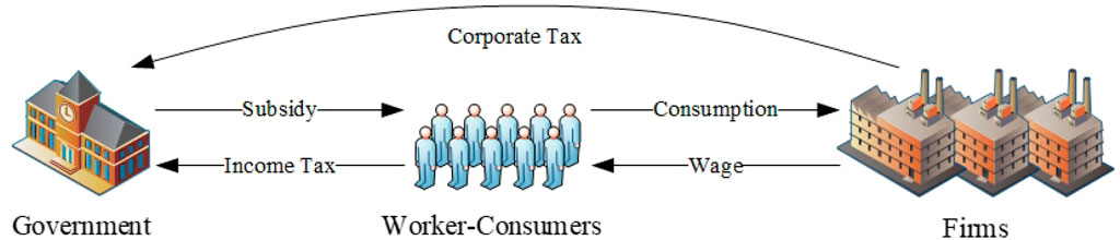
Figure 1. HMAE model. Workers earn an income by working for the firm, which they can use to purchase goods. Firms produce goods, pay workers, set prices for goods, and invest capital. The government levies wage taxes and profit taxes on workers and firms and redistributes tax revenues as subsidies to workers. Arrows represent the money flow and interrelationships between agents.

2.1 Strategy space

The strategy space represents the set of strategies that an agent can decide autonomously. Drawing on the setting of intelligent agents in related papers [54, 55], this paper defines the strategy space of workers, firms, and governments. The worker’s strategy space includes working time and consumption amount. The firm’s strategic space includes the unit price of its products, the hourly wages it pays workers, and its investment options. The government’s strategic space includes formulating tax policies such as tax brackets and tax rates, and the tax policies for workers and firms are distinct. Assuming that the HMAE model includes $NW$ workers, $NF$ firms, and a government, their strategy space can be defined as follows.

1) Worker’s strategy space. Considering the dual actions of work and consumption exhibited by workers, the model constructs the worker’s strategy space as a two-dimensional vector, denoted as $w_i=⟨H_i,C_i⟩$, where $H_i=[h_{1,i},\dots ,h_{j,i},\dots ,h_{NW,i}]$ represents the work decision of worker $i$ and $h_{j,i}\in N$ represents the working hours of worker $i$ in firm $j$. $C_i=[c_{1,i},\dots ,c_{j,i},\dots ,c_{NF,i}]$ represents the consumption decision, and $c_{j,i}\in N$ represents the quantity of goods consumed by workers in firm $j$.

2) Firm’s strategy space. Since the firm engages in three distinct behaviors, namely, hiring workers, producing goods, and making investments, we use $f_i=⟨P_j,W_j,Ca{p}_j⟩$ to represent a three-dimensional strategy space, where $P_j\in N$ represents the unit price of goods sold by firm $j$ and $W_j\in N$ represents the hourly wage paid to workers by firm $j$. $Ca{p}_j$ represents the investment behavior of firm $j$. When $Ca{p}_j=1$, the firm decides to invest in the next round, which may lead to more production of goods and higher future economic growth. On the contrary, when $Ca{p}_j=0$, firm $j$ will not invest in the next round.

3) Government’s strategy space. Based on the government’s capacity for macro tax policy formulation, the model defines its strategy space as a three-dimensional vector, denoted as $G=⟨R_w,T_w,t_f⟩$. $R_w=[r_w^1,r_w^2,\dots ,r_w^{TW}]$ represents the taxation range of individual income tax for workers. $T_w=[t_w^1,t_w^2,\dots ,t_w^{TW}]$ represents the tax rate corresponding to $R_w$, where $TW$ represents the total number of taxation range divisions. Furthermore, all firms have the same tax rate $t_f$. For example, when $R_w=[\mathrm{5,000,10,000}]$, $T_w=[0.25,0.5]$, and $t_f=0.3$, workers whose income is less than 5,000 do not need to pay tax. Workers with an income of more than 5,000 and less than 10,000 are required to pay 25% of their income as wage tax; workers with an income of more than 10,000 need to pay 50% of their income as wage tax. Meanwhile, all firms need to pay 30% of their profits as taxes.

Taking into account the real-world constraints on variables such as workers’ work hours, consumption amounts, and available quantities of goods that can be sold in the firm, we incorporate the following constraints into the model:

1) Time constraint. Since people’s available time is limited in reality, the sum of the worker’s allocated working time and consumption time needs to satisfy the maximum time constraint. Therefore, the actual working hours $h_{j,i}$ and consumption hours $c{h}_{j,i}$ of worker $i$ are used to indicate potential discrepancies with the planned working hours $h_{j,i}^{\prime }$ and consumption hours $c{h}_{j,i}^{\prime }$. The constraint relationship between $h_{j,i}$ and $c{h}_{j,i}$ needs to satisfy Equation 1.

${\displaystyle \sum _{j\in NF}}{h}_{j,i}+{\displaystyle \sum _{j\in NF}}c{h}_{j,i}⩽Tim{e}_{\mathit{thred}},(1)$

where $Tim{e}_{\mathit{thred}}$ is the threshold for the total time workers spend working and consuming. For uniform dimensions and considering the real-world scenario where longer consumption time means the opportunity to purchase more goods, the relationship between the two is set as $c{h}_{j,i}^{\prime }=c_{j,i}$, where $c_{j,i}$ represents the quantity of goods purchased by worker $i$ from firm $j$ and $c{h}_{j,i}^{\prime }$ represents the time spent by worker $i$ on shopping. Based on the reality that work is usually a fixed behavior and consumption is optional, work decisions are prioritized over consumption decisions. We discuss the computation of actual consumption and working hours in the following three cases:

Case 1: If ${\sum }_{j\in NF}{h}_{j,i}^{\prime }+{\sum }_{j\in NF}c{h}_{j,i}^{\prime }⩽Tim{e}_{\mathit{thred}}$, actual working hours $h_{j,i}$ and $c{h}_{j,i}$ can be described as Equation 2.

$\begin{array}{c}\hfill \begin{array}{c}\hfill \left\{\begin{array}{c}{h}_{j,i}=h_{j,i}^{\prime }\hfill \\ c{h}_{j,i}=c{h}_{j,i}^{\prime }\hfill \end{array}\right..\end{array}\end{array}(2)$

Case 2: If ${\sum }_{j\in NF}{h}_{j,i}^{\prime }+{\sum }_{j\in NF}c{h}_{j,i}^{\prime }⩾Tim{e}_{\mathit{thred}}$ and ${\sum }_{j\in NF}{h}_{j,i}^{\prime }<Tim{e}_{\mathit{thred}}$, the actual consumption hours $c{h}_{j,i}$ and working hours $h_{j,i}$ can be described as Equation 3.

$\begin{array}{c}\hfill \begin{array}{c}\hfill \left\{\begin{array}{c}{h}_{j,i}=h_{j,i}^{\prime }\hfill \\ c{h}_{j,i}=\frac{c{h}_{j,i}^{\prime }\cdot \left(Tim{e}_{\mathit{thred}}-{\sum }_{j\in NF}{h}_{j,i}^{\prime }\right)}{{\sum }_{j\in NF}c{h}_{j,i}^{\prime }}\hfill \end{array}\right..\end{array}\end{array}(3)$

Case 3: If ${\sum }_{j\in NF}{h}_{j,i}^{\prime }⩾Tim{e}_{\mathit{thred}}$, actual working hours $h_{j,i}$ are proportionally reduced based on the ratio in $h_{j,i}$, as shown in Equation 4.

$\begin{array}{c}\hfill \begin{array}{c}\hfill \left\{\begin{array}{c}{h}_{j,i}=\frac{h_{j,i}^{\prime }\cdot Tim{e}_{\mathit{thred}}}{{\sum }_{j\in NF}{h}_{j,i}^{\prime }}\hfill \\ c{h}_{j,i}=0\hfill \end{array}\right..\end{array}\end{array}(4)$

The working hour used in this article refers to the actual working hour.

2) Budget constraint. Budget often refers to the total amount of money a person has available for consumption. Therefore, the budget $B_{w_i}^t$ can be defined as Equation 5,

$B_{w_i}^t=B_{w_i}^{t-1}+I_{w_i}-{\displaystyle \sum _{j\in NF}}\left(c_{j,i}\cdot P_j\right),(5)$

where income $I_{w_i}$ is defined as Equation 6 and ${\delta }_i$ represents the work endowment of worker $i$.

$I_{w_i}={\delta }_i\cdot {\displaystyle \sum _{j\in NF}}\left(h_{j,i}\cdot W_j\right).(6)$

$B_{w_i}^t$ is a cumulative value that represents the total budget for workers in time step $t$, and worker consumption needs to satisfy the constraint of not exceeding their own budgets, as shown in Equation 7:

${\displaystyle \sum _{j\in NF}}\left(c_{j,i}\cdot P_j\right)⩽B_{w_i}^t,(7)$

where $P_j$ is the unit price of goods sold by firm $j$ and $c_{j,i}$ represents the actual quantity of goods purchased by worker $i$ in firm $j$. Due to budget constraints, the quantity of goods $c_{j,i}^{\prime }$ that workers attempt to purchase may not necessarily coincide with the quantity of goods $c_{j,i}$ they can actually buy, potentially resulting in a proportional reduction. The specific handling method is defined as Equation 8.

$\begin{array}{c}\hfill \begin{array}{c}\hfill c_{j,i}=\left\{\begin{array}{cc}{c}_{j,i}^{\prime },\hfill & {\displaystyle \sum _{j\in NF}}\left(c_{j,i}^{\prime }\cdot P_j\right)⩽B_{w_i}^t\hfill \\ B_{w_i}^t\frac{c_{j,i}^{\prime }}{{\sum }_{i\in NW}{c}_{j,i}^{\prime }}\frac{1}{P_j},\hfill & otherwise\hfill \end{array}\right..\end{array}\end{array}(8)$

3) Consumption constraint. The total amount of goods that all workers in firm $j$ can purchase should be less than the inventory $In{v}_j$, as shown in Equation 9.

${\displaystyle \sum _{i\in NW}}{c}_{j,i}⩽In{v}_j,(9)$

where $c_{j,i}$ represents the quantity of goods actually purchased by worker $i$ from firm $j$. If the total amount of goods $c_{j,i}^{\prime }$ that all workers expect to buy from firm $j$ exceeds the inventory quantity, it is necessary to proportionally reduce the expected purchase quantities to fit within the available inventory for sale. The actual quantity of goods $c_{j,i}$ purchased by worker $i$ from firm $j$ is expressed as Equation 10.

$\begin{array}{c}\hfill \begin{array}{c}\hfill c_{j,i}=\left\{\begin{array}{cc}{c}_{j,i}^{\prime },\hfill & {\displaystyle \sum _{i\in NW}}{c}_{j,i}^{\prime }⩽In{v}_j\hfill \\ \frac{c_{j,i}^{\prime }\cdot In{v}_j}{{\sum }_{i\in NW}{c}_{j,i}^{\prime }},\hfill & otherwise\hfill \end{array}\right..\end{array}\end{array}(10)$

2.2 Utility function

The agent’s behavior is influenced by an incentive function focusing on optimizing the overall utility. This requires the agent to seek rewards to improve performance and achieve its goals constantly [56].

1) Worker’s utility. Based on the worker’s work and consumption decisions, the utility function of worker $i$ consists of consumption utility, work expense, and commuting expense, as shown in Equation 11:

$u\left(x_i\right)=\frac{{\left({\sum }_{j\in NF}{c}_{j,i}+1\right)}^{1-\eta }-1}{1-\eta }-{\theta }_i{\displaystyle \sum _{j\in NF}}{h}_{j,i}-{\displaystyle \sum _{j\in NF}}\left(d_{j,i}\cdot h_{j,i}\right).(11)$

a) Consumption happiness. The constant relative risk aversion (CRRA) function plays an important role in the calculation of consumption utility and is a common tool used to describe the happiness derived from workers’ consumption patterns [57, 58]. Here, we use the CRRA utility function $\frac{{({\sum }_{j\in NF}{c}_{j,i}+1)}^{1-\eta }-1}{1-\eta }$ to depict the impact of consumption on the happiness of workers, where the coefficient $\eta$ ($\eta >0$ and $\eta \ne 1$) represents the impact of consumption on the worker’s happiness. The larger the value of $\eta$, the greater the growth rate of worker happiness as the purchase quantity increases. As the value of $\eta$ increases, the magnitude of the increase (resp., decrease) in worker happiness intensifies with the corresponding increase (resp., decrease) in the quantity of purchased goods.

b) Work expense. Work expenses represent the negative impact of working hours on workers’ happiness, expressed as ${\theta }_i{\sum }_{j\in NF}{h}_{j,i}$, where ${\theta }_i\in [\mathrm{0,1}]$ represents varying degrees of reluctance to work. The larger the ${\theta }_i$, the greater the negative impact of working hours on the workers’ sense of happiness. Furthermore, due to the heterogeneity of work endowments, workers make different decisions and choices regarding work and consumption, which leads to differences in their perception of work expense.

c) Commuting expense. The introducing of spatial information requires workers to consider commuting expenses when calculating utility values. The commuting distance from residence to work is a critical factor in employment decision-making, that is, the longer the commuting distance, the lower the worker’s happiness at work. Therefore, the commuting expense can be described as ${\sum }_{j\in NF}(d_{j,i}\cdot h_{j,i})$, where $d_{j,i}$ represents the commuting distance of worker $i$ to firm $j$.

2) Firm’s utility. Based on the firm’s strategy space, the utility function of firm $j$ contains sales profit, salary expense, investment expense, and tax expense, denoted as Equation 12.

$v\left(y_j\right)={\displaystyle \sum _{i\in NW}}\left(c_{j,i}^{\prime }\cdot P_j\right)-{\displaystyle \sum _{i\in NW}}\left(h_{j,i}\cdot W_j\right)-ca{p}_j-CTa{x}_j.(12)$

a) Sales profit. Because selling goods brings profit to firms, the quantity of goods sold is positively related to the revenue generated. ${\sum }_{i\in NW}(c_{j,i}^{\prime }\cdot P_j)$ represents the sales profit, where ${\sum }_{i\in NW}{c}_{j,i}^{\prime }$ and $P_j$ represent the quantity and unit price of goods sold by firm $j$, respectively.

b) Salary expense. Since producing goods requires human resources, firms need to pay the cost of hiring labor. We use ${\sum }_{i\in NW}(h_{j,i}\cdot W_j)$ to represent the labor compensation, where ${\sum }_{i\in NW}{h}_{j,i}$ indicates the total hours worked by all workers and $W_j$ represents the hourly wage in firm $j$.

c) Investment expense. There is a positive relationship between investment and utility, that is, increased investment helps increase the output of commodity production and can promote the future economic growth. The precise expression for the utility function is shown in Equation 13.

$ca{p}_j=B_{f_j}\cdot rat{e}_{Ca{p}_j}\cdot Ca{p}_j,(13)$

where $B_{f_j}$ represents the budget of firm $j$. $Ca{p}_j\in \{\mathrm{0,1}\}$ represents the firm’s investment decisions. If $Ca{p}_j=1$, firm $j$ will invest in the next iteration; if $Ca{p}_j=0$, then firm $j$ will not invest. Using its capital $ca{p}_j$ and labor force ${\sum }_{j\in NF}{h}_{j,i}$, the total number of goods $P_j$ that firm $j$ can produce can be modeled as Equation 14.

$P_j={ca{p}_j}^{1-\alpha }\cdot {{\displaystyle \sum _{j\in NF}}{h}_{j,i}}^{\alpha },(14)$

where $\alpha \in [\mathrm{0,1}]$ represents the importance of capital relative to labor.

d) Tax expense. According to the government’s tax policy $T_f$, the amount of tax paid by a firm is based on its sales revenue, as shown in Equation 15.

$CTa{x}_j=\left({\displaystyle \sum _{i\in NW}}{c}_{j,i}\cdot P_j\right)\cdot T_f.(15)$

3) Government’s utility. To assess the health of a country’s economy [59], governments often use GDP, which measures the market value of all final goods and services produced during a specific time period [60], and the Gini coefficient, which measures the income disparity among residents [58, 61]. Therefore, the GDP, Gini coefficient, or their combination can be used to characterize the government’s utility.

2.3 Updating mechanism

It is known that people tend to interact more frequently with others who possess similar knowledge [62]. Therefore, in the case of limited rationality and incomplete information acquisition, learning from neighbors is a feasible way to update the strategy to maximize the utility value. To increase randomness for exploring diverse solutions or seeking the global optimum, the updating mechanism is divided into two processes: exploration and learning.

1) The strategy update of the worker. To update the working and consumption strategies aiming for higher utility values, worker $i$ randomly selects a neighbor $i^{\prime }$ within a spatial range as the target for strategy learning. The pseudo-code of the worker’s updating mechanism is shown in Algorithm 1. If $u(w_i)\ge u(w_{i^{\prime }})$, $i$ keeps its own strategy unchanged (lines 1–2). Otherwise, worker $i$ enters the exploration stage with probability $p$ and randomly updates its strategy (lines 4–5) or enters the learning stage with probability $1-p$ and updates its strategy according to Equation 16 by imitating the strategy of neighbor $i^{\prime }$ (lines 6–7).

$\begin{array}{c}\hfill \begin{array}{c}\hfill \left\{\begin{array}{c}{H}_i={\displaystyle \sum _{j\in NF}}[h_{j,i}+\left(h_{j,i^{\prime }}-h_{j,i}\right)\cdot l{r}_w]\hfill \\ C_i={\displaystyle \sum _{j\in NF}}[c_{j,i}+\left(c_{j,i^{\prime }}-c_{j,i}\right)\cdot l{r}_w],\hfill \end{array}\right.\end{array}\end{array}(16)$

where $H_i=[h_{1,i},\dots ,h_{j,i},\dots ,h_{NW,i}]$ represents the work decision of worker $i$ and $h_{j,i}\in N$ represents the working hours of worker $i$ in firm $j$. $C_i=[c_{1,i},\dots ,c_{j,i},\dots ,c_{NF,i}]$ represents the consumption decision, and $c_{j,i}\in N$ represents the quantity of goods consumed by the worker in firm $j$. $l{r}_w$ represents the worker’s learning rate.

The probability $p$ is defined as $P_w-\frac{t}{ExploreTime}$, aiming to explore with a greater probability in the early stage and to update the strategy with the goal of maximizing the utility value in the later stages. $P_w$ represents the initial exploration probability, $t$ represents the current round, and $ExploreTime$ stands for the number of explorations.

Algorithm 1.The strategy update of the worker.

Require: Time step $t$, worker $i$, neighbor $i^{\prime }$, utility function $u$, imitate probability $P_w$, learning rate $l{r}_w$, exploration time $ExploreTime$, and random number $p\in [\mathrm{0,1}]$;

Ensure: Working hours $H_i$ and consumption quantities $C_i$

1: if $u(w_i)>u(w_{i^{\prime }})$ then

2:  the worker $i$ keeps its own strategy unchanged;

3: else

4:  if $p\le P_w-\frac{t}{ExploreTime}$ then//in the exploration phase

5:   the worker i randomly chooses working hours $H_i$ and consumption quantities $C_i$;

6:  else//in the learning phase

7:   the worker $i$ imitates the strategy of the selected neighbor $i^{\prime }$ using Equation 16;

8:  end if

9: end if

10: return strategy $x_i=⟨H_i,C_i⟩$;

2) The strategy update of the firm. The firm’s renewal process is similar to that of the worker’s. In order to update the unit price of goods, workers’ hourly wage, and investment decisions, firm $j$ randomly selects a neighbor $j^{\prime }$ as the target for strategy learning. The pseudo-code of the learning stage is shown in Algorithm 2. If $u(f_j)⩾u(f_{j^{\prime }})$, firm $j$ keeps its own strategy unchanged (lines 1–2). Otherwise, firm $j$ has a probability of $q$ to enter the exploration stage (lines 4–5) and a probability of $1-q$ to enter the learning stage (lines 6–7). To increase the exploration probability in the early stages and guide later updates toward utilizing optimized strategies, $q=P_f-\frac{t}{ExploreTime}$ is set. In the exploration process, firm $j$ randomly updates its strategies for the unit price of goods, workers’ hourly wage, and investment decisions (line 5). In the learning process, firm $j$ imitates the strategy of neighbor $j^{\prime }$ with the learning rate $l{r}_f$ through Equation 17 (line 7).

$\begin{array}{c}\hfill \begin{array}{c}\hfill \left\{\begin{array}{c}{P}_j=P_j+\left(P_{j^{\prime }}-P_j\right)\cdot l{r}_f\hfill \\ W_j=W_j+\left(W_{j^{\prime }}-W_j\right)\cdot l{r}_f\hfill \\ Ca{p}_j=Ca{p}_{j^{\prime }}\hfill \end{array}\right..\end{array}\end{array}(17)$

Algorithm 2.The strategy update of the firm.

Require: Time step $t$, firm $j$, firm $j^{\prime }$, utility function $v$, imitate probability $P_f$, learning rate $l{r}_f$, and random number $q\in [\mathrm{0,1}]$;

Ensure:Unit price $P_j$, hourly wage $W_j$, and investment decision $Ca{p}_j$

1: if $v(f_j)>v(f_{j^{\prime }})$, then

2:  the firm $j$ keeps its own strategy unchanged;

3: else

4:  if $q\le P_f-\frac{t}{ExploreTime}$ then//in the exploration phase

5:   the firm j randomly chooses unit price $P_j$, hourly wage $W_j$, and investment decision $Ca{p}_j$;

6:  else//in the learning phase

7:   the firm $j$ imitates the strategy of the selected neighbor $j^{\prime }$ using Equation 17;

8:  end if

9: end if

10: return strategy $y_j=⟨P_j,W_j,Ca{p}_j⟩$;

3) The strategy update of the government. Since we focus on the economic evolution and phenomenon emergence under fixed tax rates and taxation ranges, the government’s tax policy will not change subsequently, that is, the government decision is not considered in this paper.

3 Experiments

In this section, we conduct simulation experiments using real data based on the HMAE model to study the emergent economic phenomena that occur during agent interaction. These experiments prove that when workers are heterogeneous at the micro-level (e.g., laziness, individual endowments, and commuting distance), workers’ work and consumption decisions will continuously update and iterate, explaining the evolution of macroeconomic phenomena in real life. All simulation experiments were executed on a Linux server equipped with an Intel(R) Xeon(R) Gold 6248R running at 3.00 GHz and 754 GB of memory. Each measurement represents the average of 10 instances.

3.1 Experimental settings

We construct a small economic society consisting of 15,000 workers and 10 firms to study the micro-level reasons behind emergent economic phenomena. We take China’s tax policy as an example to conduct a simulation experiment and set the government’s tax rate for all firms to $T_f=0.25$. The government’s tax range for workers is $R_w=[\mathrm{5,000,8,000,17,000,30,000,40,000,60,000,85,000}]$, and the corresponding tax rate is $T_w=[0.03,0.1,0.2,0.25,0.3,0.35,0.45]$. The learning probability of both workers and firms is 0.1, and the learning rate is 0.05. All parameters are shown in Table 1.

Table 1

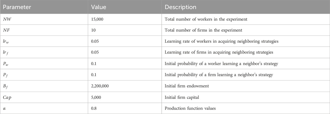
Table 1. Experiment parameter settings.

To deeply explore the reasons behind the impact of worker heterogeneity on economic phenomena and better fit the income distribution of residents, we divide workers into three categories based on laziness factors: hard, normal, and lazy. These three categories of workers account for 20%, 60%, and 20% of the total number of workers, respectively. At the same time, considering the heterogeneity of work efficiency in real-world scenarios, workers can also be divided into four types based on their work endowments [63, 64], accounting for 40%, 40%, 15%, and 5% of the total number of workers, respectively. This paper combines the existing population income distribution research [65–67] and provides the final parameter values after data fitting and parameter adjustment (see Table 2 for details). Finally, 12 categories of workers are formed considering laziness factors and work endowment.

Table 2

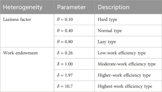
Table 2. Worker heterogeneity setting.

To further explore the impact of commuting distance on workers’ strategic choices, we obtained the points of interest (POI) data on Hangzhou City, Zhejiang Province, from AMAP (http://www.amap.com/). We filtered workers’ residence and firm locations and then constructed the spatial location relationship between them, as shown in Figure 2A. To simplify data analysis and facilitate the discovery of underlying emergent phenomena, we used the K-means method [68, 69] and selected cluster centroids as representative locations of workers and firms, as shown in Figure 2B.

Figure 2

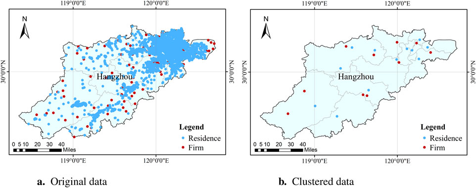
Figure 2. Residential and firm location distributions. (A) Original location distributions for residence areas and firms, where red represents firms and blue represents residence areas. (B) Clustered location distributions for firms and residence areas in the experiment.

3.2 Experimental results

In this section, we analyze the reasons behind emerging economic phenomena by analyzing the evolution of behavioral attributes of workers and firms. Specifically, the behavioral evolution of workers is analyzed from the aspects of working hour, income, consumption, and commuting distance, and the behavioral evolution of firms is analyzed from the unit price of products sold and hourly wage. Since there is a certain degree of uncertainty in the initial strategy learning of the agent, we conducted 10 experiments on different parameters and took the average to minimize the impact of early experimental disturbances on the experimental results. The number of simulation experiment steps is set to 1,000 to ensure that the experimental results demonstrate convergence.

3.2.1 Experiment on the dynamic evolution of worker behavior

Work and consumption are workers’ two main decision-making behaviors and play a crucial role in the evolution of workers’ behavior. We analyze the dynamic behavioral evolution of workers from several aspects, such as their working hours, wage income, consumption amount, and commuting distance to work choices.

We analyze the evolution trend of working hours for 12 types of heterogeneous workers, as shown in Figure 3. Figure 3A shows that when the workers’ endowments are the same, the working hours of hard-type workers exceed the working hours of normal and lazy-type workers. For instance, when the workers are all low-efficiency types $(\delta =0.26)$, the working time curve of hard-type workers $(\theta =0.10)$ is higher than that of other workers. This phenomenon can be explained by Equation 11: the more significant the laziness factor, the greater the negative impact of working time on worker happiness and the lower the workers’ utility value. Therefore, people who work harder will devote more working hours to work, which can further weaken the negative relationship between working time and workers’ utility value and, at the same time, promote the improvement in workers’ willingness to work. The result is consistent with real-life common knowledge that lazy workers tend to devote fewer hours to their jobs [70, 71]. Additionally, when the laziness factor is consistent, workers with a work endowment of $\delta =0.26$ exhibit longer working hours than workers with other endowments.

Figure 3

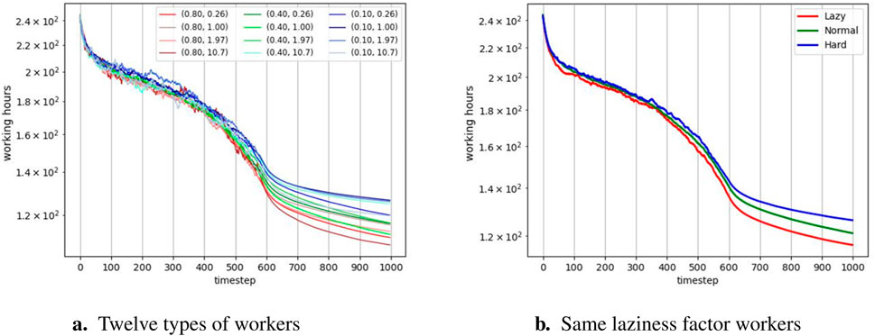
Figure 3. Evolution of average working hours. (A) Evolution of average working hours for 12 types of workers. The vector set in the legend represents $(\theta ,\delta )$. For example, $(0.80,0.26)$ represents the laziness factor $\theta =0.80$ and the endowment of work $\delta =0.26$. (B) Evolution of the average working hours for the same group of laziness factors.

In order to further verify the impact of laziness factors on workers’ working hours, we calculate the average working time of workers under each laziness factor, as shown in Figure 3B. The experimental results show that the average working hours of hard-type workers are higher than those of normal-type workers, and the average working hours of lazy-type workers are the lowest, further confirming the conclusion that the laziness mentioned above affects workers’ working hours. Since workers’ decisions have a certain degree of randomness in the exploration stage, the evolution curve of working time oscillates in the early stage. In addition, because working hours are negatively related to workers’ utility value, workers’ overall working hours show a downward trend over time. Therefore, driven by the goal of utility maximization, the time workers invest gradually decreases over time.

3.2.1.1 Dynamic evolution of income

Workers’ income is closely related to their working hours and work endowments, playing a crucial role in studying the effects on workers’ budgets and consumption. Because workers’ income is positively correlated with working hours and workers’ working hours are generally on a downward trend (Figure 3), workers’ income is also on a downward trend overall, as shown in Figure 4.

Figure 4

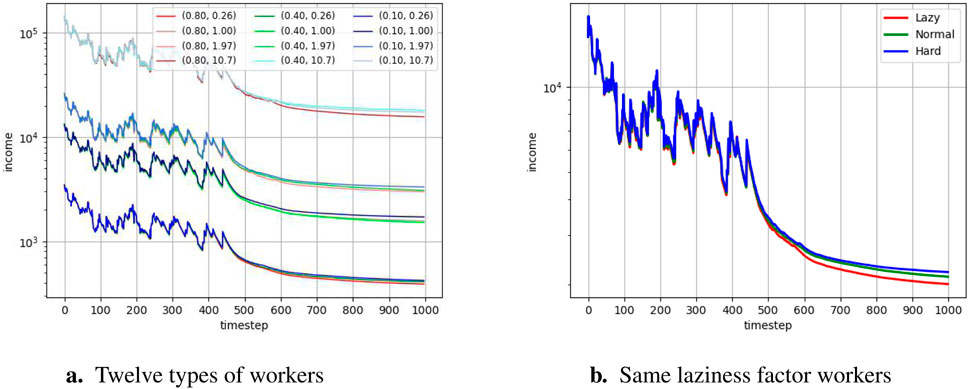
Figure 4. Evolution of the mean income. (A) Evolution of income for 12 types of workers. (B) Evolution diagram of the mean income of the same laziness factor group.

Figure 4A shows that the workers’ income curve presents four obvious distribution categories, and the correspondence between these four categories and their endowments is consistent. Moreover, each category has a similar pattern, with hard workers earning the highest wages, and lazy workers earning the lowest. These emergent phenomena, which are ultimately manifested through individuals, show a clear positive correlation between work endowment and workers’ income. When the laziness factor is the same, the income of workers with endowment $\delta =10.7$ is higher than that of workers with other endowments. Workers with higher work endowments have longer effective working hours and higher incomes.

To further verify the impact of laziness factors on workers’ income, we calculate the average income of workers with the same laziness factors, as shown in Figure 4B. It can be seen that the income of different types of workers from high to low is hard, normal, and lazy, which further confirms the conclusion that a lower laziness factor may bring a higher income. It also reflects that lazy workers are less engaged, invest less time, and earn less [71]. Additionally, the evolution of income shows early oscillations and an overall downward trend, which is also related to a certain randomness in workers’ decision-making during the exploration stage.

3.2.1.2 Dynamic evolution of consumption

Consumption is a vital decision-making behavior for workers, significantly affecting their happiness and work utility values. As workers’ incomes are on a downward trend, their budgets for purchasing goods also decrease, resulting in a downward trend in consumption, as shown in Figure 5. Figure 5A shows the evolution of the consumption amount of 12 categories of workers. It can be seen that when the endowments of workers are the same, the consumption amount of normal-type workers exceeds that of hard and lazy-type workers. For instance, when workers are all low-efficiency types ($\delta$ = 10.7), the consumption amount curve of normal-type workers ($\theta$ = 0.40) is higher than that of other workers. This phenomenon can be explained using Equation 1 combined with Figure 3B. Since working hours and consumption hours are negatively correlated under time constraints, when the budget is sufficient, hard-type workers spend slightly less time on consumption than normal-type workers.

Figure 5

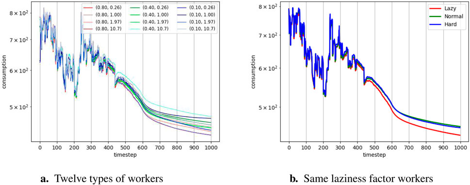
Figure 5. Evolution of mean consumption. (A) Evolution of consumption for 12 types of workers. (B) Evolution diagram of the mean consumption of the same laziness factor group.

Figure 5B further explores the impact of the laziness factor on consumption, revealing that normal-type workers have the highest consumption amount, followed by hard-type workers, while lazy-type workers have the lowest consumption amount. Taking the above conclusions into consideration, we can see that normal-type workers work moderate hours and have sufficient budget and consumption time, making them the highest consuming group.

3.2.1.3 The impact of commuting distance on working behaviors

In addition to heterogeneity in endowment and laziness factors, workers living in different regions also have different commuting distances to reach firms, leading to differing commuting expenses that affect utility values and workers’ choices of firms in different locations. As shown in Figure 6, we randomly select a residential area to analyze the relationship between the commuting distance and workers’ willingness to choose firms. Similar phenomena can be observed in other residential areas. Figure 6A shows the distribution of working hours in various firms for all workers in the selected residential area. As commuting distances increase, workers’ working hours gradually decrease. Combining Equation 11 can explain this phenomenon: the longer the commuting distance, the higher the commuting cost, which will negatively impact the utility value. Therefore, workers tend to choose firms closer to their residences.

Figure 6

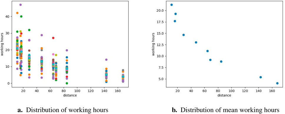
Figure 6. Distribution of working hours among workers in 10 firms. The x-axis represents the commuting distance to 10 different companies for all workers living in residential areas, measured in kilometers. The y-axis represents working hours, measured in hours. Points of the same color represent the time distribution of the same worker in different firms. (A) Statistical distribution of working hours for all workers from the residential area across different firms. (B) Average working hour distribution of all workers across each firm.

In order to more clearly explore the impact of commuting distance on workers’ willingness to work, we display the average working hours of workers in each firm, as shown in Figure 6B. As the commuting distance from residential areas to firms increases, the working hours that workers are willing to spend show a decreasing trend.

3.2.2 Experiment on the dynamic evolution of firm behavior

Setting the unit price of goods and the hourly wage paid to workers are two critical firm decisions. In this section, we analyze these two decisions to understand the dynamic behavioral evolution of the firm.

3.2.2.1 Dynamic evolution of the unit price

We analyze the evolution of the unit price of each firm’s products over time, as shown in Figure 7. The products of all firms are homogeneous, and the unit prices of these products will eventually converge to a unified equilibrium value after a period of fluctuation. Equation 12 shows that there is a positive correlation between the utility value of firms and sales profits. Therefore, firms will strive to increase the unit price of goods to maximize profits. If the unit price of goods is set excessively high, workers’ expenditure may not be enough to support their desired consumption, affecting the sales quantity of the goods. On the contrary, if the product’s unit price is set uncompetitively low, it will reduce the total sales price of the product, thereby affecting the utility value of the firm. Over time, the market moves toward uniform unit prices for goods to strike a balance between maximizing corporate goals and meeting the daily needs of workers. Therefore, under the premise of product homogeneity, after the dynamic adjustment of product prices in the early stage of the market, the unit prices of the firm’s products will eventually become consistent [72, 73].

Figure 7

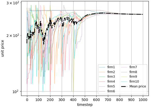
Figure 7. Unit price of goods. Each line in the figure represents the unit price of a firm’s goods.

3.2.2.2 Dynamic evolution of hourly wage

Figure 8 shows the evolution trend of firms hourly wages. Hourly wages in all firms converge to a consistent equilibrium value after an initial period of fluctuation. It is worth noting that this evolution eventually converges to a relatively low value. According to Equation 12, a firm’s utility value is negatively related to wage expenditures. Therefore, firms will continue to increase profits by lowering hourly wages, reducing wages paid to workers, and maximizing their utility value. In addition, workers rely on the wages they earn from working in firms to meet their daily needs and need sufficient consumption to enhance their happiness. Over time, the firm’s hourly wage eventually develops to the equilibrium point where it balances its profit purposes with the workers’ basic income needs. However, since working hours of workers show a downward trend with iteration (Figure 3B), they partially affect workers’ willingness to work. Affected by this, the average hourly wages of workers have also shown a corresponding downward trend.

Figure 8

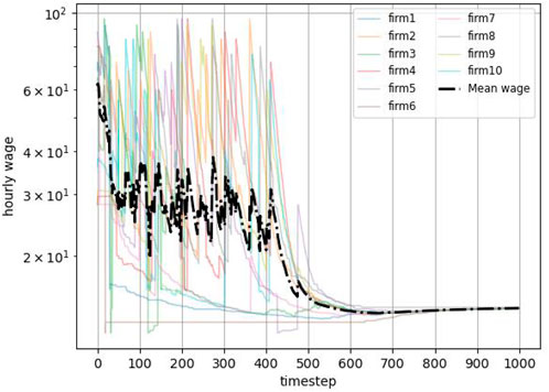
Figure 8. Hourly wage. Each line in the figure represents the hourly wage of a firm.

4 Conclusion

In this paper, we proposed a high-fidelity multi-agent economic model that focuses on the heterogeneity of individuals at the micro-level to explore the reasons behind the emergence of economic phenomena. Additionally, we investigated the impact of spatial distance on workers’ willingness to work. We studied the evolutionary processes of behavioral decision-making for both workers and firms through experiments. From the workers’ perspective, their work and consumption decisions show an apparent evolutionary trend under the influence of heterogeneous laziness factors and work endowment. Workers with higher work efficiency tend to have more time and income for consumption. Moreover, workers with lower laziness factors lean toward investing more time in work. From the firm’s perspective, the evolution of both unit prices for goods and hourly wages eventually develops to the equilibrium point that balances the firms’ profits and the livelihood needs of the workers. These emerging experimental results are consistent with observations of economic phenomena in the real world, and the HMAE method provides us with a new tool to study social phenomena from a microscopic perspective. In the future, we will consider proposing complex models by characterizing intelligent agents with more diversity and heterogeneity to predict potential economic phenomena and infer social development patterns. For example, we can further refine our understanding of the workforce by characterizing workers’ age, employability, and preferences. This allows us to delve into the intricacies of economic evolution from various dimensions, including familial context. Additionally, expanding the scope to encompass diverse firm types will enrich our research on the dynamics of competition and cooperation within the business landscape. By integrating agents representing external markets into our model, we can study the impact of export price changes on domestic market stability.

Data availability statement

The raw data supporting the conclusion of this article will be made available by the authors, without undue reservation.

Author contributions

CW: writing–original draft, visualization, methodology, funding acquisition, formal analysis, and conceptualization. XM: writing–original draft, visualization, software, methodology, and conceptualization. XJ: writing–review and editing, methodology, funding acquisition, formal analysis, and conceptualization. HZ: writing–review and editing and software. ZW: writing–review and editing, funding acquisition, formal analysis, and conceptualization.

Funding

The author(s) declare that financial support was received for the research, authorship, and/or publication of this article. This work was supported by the Zhejiang Provincial Natural Science Foundation of China (LTGG24D010003 and LTGG23F030004) and the National Natural Science Foundation of China (42201510).

Conflict of interest

The authors declare that the research was conducted in the absence of any commercial or financial relationships that could be construed as a potential conflict of interest.

Publisher’s note

All claims expressed in this article are solely those of the authors and do not necessarily represent those of their affiliated organizations, or those of the publisher, the editors, and the reviewers. Any product that may be evaluated in this article, or claim that may be made by its manufacturer, is not guaranteed or endorsed by the publisher.

References

1. Tesfatsion L. Agent-based computational economics: a constructive approach to economic theory. Handbook Comput Econ (2006) 2:831–80. doi:10.1016/S1574-0021(05)02016-2

CrossRef Full Text | Google Scholar

2. Limburg KE, O’Neill RV, Costanza R, Farber S. Complex systems and valuation. Ecol Econ (2002) 41:409–20. doi:10.1016/s0921-8009(02)00090-3

CrossRef Full Text | Google Scholar

3. Arthur WB. Complexity and the economy. science (1999) 284:107–9. doi:10.1126/science.284.5411.107

PubMed Abstract | CrossRef Full Text | Google Scholar

4. Arthur WB. Foundations of complexity economics. Nat Rev Phys (2021) 3:136–45. doi:10.1038/s42254-020-00273-3

PubMed Abstract | CrossRef Full Text | Google Scholar

5. Ramalingam B, Jones H, Reba T, Young J. Exploring the science of complexity: ideas and implications for development and humanitarian efforts, 285. London: Overseas Development Institute (2008).

Google Scholar

6. Kuhn JR, Courtney JF, Morris B, Tatara ER. Agent-based analysis and simulation of the consumer airline market share for frontier airlines. Knowledge-Based Syst (2010) 23:875–82. doi:10.1016/j.knosys.2010.06.002

CrossRef Full Text | Google Scholar

7. Heylighen F. The science of self-organization and adaptivity. encyclopedia Life support Syst (2001) 5:253–80.

Google Scholar

8. George DA, Lin BC-a., Chen Y. A circular economy model of economic growth. Environ Model and Softw (2015) 73:60–3. doi:10.1016/j.envsoft.2015.06.014

CrossRef Full Text | Google Scholar

9. Irwin EG, Geoghegan J. Theory, data, methods: developing spatially explicit economic models of land use change. Agric Ecosyst and Environ (2001) 85:7–24. doi:10.1016/s0167-8809(01)00200-6

CrossRef Full Text | Google Scholar

10. Morgan MS. The world in the model: how economists work and think. Cambridge University Press (2012).

Google Scholar

11. Bautista RM. Macroeconomic models for east asian developing countries. Asian-Pacific Econ Lit (1988) 2:1–25. doi:10.1111/j.1467-8411.1988.tb00198.x

CrossRef Full Text | Google Scholar

12. Capros P, Karadeloglou P, Mentzas G. An empirical assessment of macroeconometric and cge approaches in policy modeling. J Pol Model (1990) 12:557–85. doi:10.1016/0161-8938(90)90013-5

CrossRef Full Text | Google Scholar

13. Farmer JD, Foley D. The economy needs agent-based modelling. Nature (2009) 460:685–6. doi:10.1038/460685a

PubMed Abstract | CrossRef Full Text | Google Scholar

14. Stiglitz JE. Where modern macroeconomics went wrong. Oxford Rev Econ Pol (2018) 34:70–106. doi:10.1093/oxrep/grx057

CrossRef Full Text | Google Scholar

15. Sims CA. Macroeconomics and reality. Econometrica: J Econometric Soc (1980) 48:1–48. doi:10.2307/1912017

CrossRef Full Text | Google Scholar

16. Geurts M, Box GEP, Jenkins GM. Time series analysis: forecasting and control. JMR, J Marketing Res (1977) 14:269. doi:10.2307/3150485

CrossRef Full Text | Google Scholar

17. Çakır MY, Kabundi A. Trade shocks from bric to South Africa: a global var analysis. Econ Model (2013) 32:190–202. doi:10.1016/j.econmod.2013.02.010

CrossRef Full Text | Google Scholar

18. Harvey AC. Estimating regression models with multiplicative heteroscedasticity. Econometrica: J Econometric Soc (1976) 44:461–5. doi:10.2307/1913974

CrossRef Full Text | Google Scholar

19. Engle RF, Granger CW. Co-integration and error correction: representation, estimation, and testing. Econometrica: J Econometric Soc (1987) 55:251–76. doi:10.2307/1913236

CrossRef Full Text | Google Scholar

20. Johansen S. Statistical analysis of cointegration vectors. J Econ Dyn Control (1988) 12(2-3):231–54. doi:10.1016/0165-1889(88)90041-3

CrossRef Full Text | Google Scholar

21. Pfleiderer P. Chameleons: the misuse of theoretical models in finance and economics. Economica (2020) 87:81–107. doi:10.1111/ecca.12295

CrossRef Full Text | Google Scholar

22. Woodford M. Optimal interest-rate smoothing. Rev Econ Stud (2003) 70:861–86. doi:10.1111/1467-937x.00270

CrossRef Full Text | Google Scholar

23. Galí J, Gambetti L. The effects of monetary policy on stock market bubbles: some evidence. Am Econ J Macroeconomics (2015) 7:233–57. doi:10.1257/mac.20140003

CrossRef Full Text | Google Scholar

24. Paccagnini A (2009). Model validation in the dsge approach: a survey. Tech. rep., working paper. Italy: Università Bocconi in Milano.

Google Scholar

25. Reis R. Is something really wrong with macroeconomics? Oxford Rev Econ Pol (2018) 34:132–55. doi:10.1093/oxrep/grx053

CrossRef Full Text | Google Scholar

26. Haldane AG, Turrell AE. An interdisciplinary model for macroeconomics. Oxford Rev Econ Pol (2018) 34:219–51. doi:10.1093/oxrep/grx051

CrossRef Full Text | Google Scholar

27. Roozmand O, Ghasem-Aghaee N, Hofstede GJ, Nematbakhsh MA, Baraani A, Verwaart T. Agent-based modeling of consumer decision making process based on power distance and personality. Knowledge-Based Syst (2011) 24:1075–95. doi:10.1016/j.knosys.2011.05.001

CrossRef Full Text | Google Scholar

28. Farmer JD, Gallegati M, Hommes C, Kirman A, Ormerod P, Cincotti S, et al. A complex systems approach to constructing better models for managing financial markets and the economy. Eur Phys J Spec Top (2012) 214:295–324. doi:10.1140/epjst/e2012-01696-9

CrossRef Full Text | Google Scholar

29. Blanchard O. On the future of macroeconomic models. Oxford Rev Econ Pol (2018) 34:43–54. doi:10.1093/oxrep/grx045

CrossRef Full Text | Google Scholar

30. Caballero RJ. Macroeconomics after the crisis: time to deal with the pretense-of-knowledge syndrome. J Econ Perspect (2010) 24:85–102. doi:10.1257/jep.24.4.85

CrossRef Full Text | Google Scholar

31. Harting P (2015). Stabilization policies and long term growth: policy implications from an agent-based macroeconomic model.

Google Scholar

32. Dawid H, Harting P, Neugart M. Fiscal transfers and regional economic growth. Rev Int Econ (2018) 26:651–71. doi:10.1111/roie.12317

CrossRef Full Text | Google Scholar

33. Assenza T, Gatti DD. E pluribus unum: macroeconomic modelling for multi-agent economies. J Econ Dyn Control (2013) 37:1659–82. doi:10.1016/j.jedc.2013.04.010

CrossRef Full Text | Google Scholar

34. Guerini M, Moneta A. A method for agent-based models validation. J Econ Dyn Control (2017) 82:125–41. doi:10.1016/j.jedc.2017.06.001

CrossRef Full Text | Google Scholar

35. Gatti DD, Di Guilmi C, Gaffeo E, Giulioni G, Gallegati M, Palestrini A. A new approach to business fluctuations: heterogeneous interacting agents, scaling laws and financial fragility. J Econ Behav and Organ (2005) 56:489–512. doi:10.1016/j.jebo.2003.10.012

CrossRef Full Text | Google Scholar

36. Gatti D, Gaffeo E, Gallegati M, Giulioni G, Palestrini A. Emergent macroeconomics: an agent-based approach to business fluctuations. Springer Science and Business Media (2008).

Google Scholar

37. Tesfatsion L. Agent-based computational economics: growing economies from the bottom up. Artif Life (2002) 8:55–82. doi:10.1162/106454602753694765

PubMed Abstract | CrossRef Full Text | Google Scholar

38. Gualdi S, Tarzia M, Zamponi F, Bouchaud J-P. Tipping points in macroeconomic agent-based models. J Econ Dyn Control (2015) 50:29–61. doi:10.1016/j.jedc.2014.08.003

CrossRef Full Text | Google Scholar

39. Caiani A, Godin A, Caverzasi E, Gallegati M, Kinsella S, Stiglitz JE. Agent based-stock flow consistent macroeconomics: towards a benchmark model. J Econ Dyn Control (2016) 69:375–408. doi:10.1016/j.jedc.2016.06.001

CrossRef Full Text | Google Scholar

40. Dawid H, Gemkow S, Harting P, Neugart M. Labor market integration policies and the convergence of regions: the role of skills and technology diffusion. The Two Sides Innovation: Creation Destruction Evol Capitalist Economies (2013) 167–86. doi:10.1007/978-3-319-01496-8_9

CrossRef Full Text | Google Scholar

41. Ponta L, Raberto M, Teglio A, Cincotti S. An agent-based stock-flow consistent model of the sustainable transition in the energy sector. Ecol Econ (2018) 145:274–300. doi:10.1016/j.ecolecon.2017.08.022

CrossRef Full Text | Google Scholar

42. Lynch C, Sermanet P. Language conditioned imitation learning over unstructured data. arXiv preprint arXiv:2005.07648 (2020). doi:10.48550/arXiv.2005.07648

CrossRef Full Text | Google Scholar

43. Suglia A, Gao Q, Thomason J, Thattai G, Sukhatme G. Embodied bert: a transformer model for embodied, language-guided visual task completion (2021). arXiv preprint arXiv:2108.04927.

Google Scholar

44. Hill F, Mokra S, Wong N, Harley T. Human instruction-following with deep reinforcement learning via transfer-learning from text (2020). arXiv preprint arXiv:2005.09382.

Google Scholar

45. Yaman A, Leibo JZ, Iacca G, Wan Lee S. The emergence of division of labour through decentralized social sanctioning. Proc R Soc B (2023) 290:20231716. doi:10.1098/rspb.2023.1716

PubMed Abstract | CrossRef Full Text | Google Scholar

46. Lindgren K. Evolutionary phenomena in simple dynamics. Artif Life (1991) 10:295–312.

Google Scholar

47. Amiti M, Pissarides CA. Trade and industrial location with heterogeneous labor. J Int Econ (2005) 67:392–412. doi:10.1016/j.jinteco.2004.09.010

CrossRef Full Text | Google Scholar

48. Coniglio ND. Regional integration and migration: an economic geography model with heterogeneous labour force. Scotland, United Kingdom: University of Glasgow (2002).

Google Scholar

49. Hayashi Y, Hsieh M-H, Setiono R. Understanding consumer heterogeneity: a business intelligence application of neural networks. Knowledge-Based Syst (2010) 23:856–63. doi:10.1016/j.knosys.2010.05.010

CrossRef Full Text | Google Scholar

50. Brock JM. Unfair inequality, governance and individual beliefs. J Comp Econ (2020) 48:658–87. doi:10.1016/j.jce.2020.03.001

CrossRef Full Text | Google Scholar

51. Dawson HJ, Fouksman E. Labour, laziness and distribution: work imaginaries among the south african unemployed. Africa (2020) 90:229–51. doi:10.1017/s0001972019001037

CrossRef Full Text | Google Scholar

52. Maltz A. Exogenous endowment—endogenous reference point. Econ J (2020) 130:160–82. doi:10.1093/ej/uez044

CrossRef Full Text | Google Scholar

53. Nguyen V-Q. Endowment-regarding preferences. J Math Econ (2021) 94:102454. doi:10.1016/j.jmateco.2020.102454

CrossRef Full Text | Google Scholar

54. Danthine JP, Donaldson JB. Methodological and empirical issues in real business cycle theory. Eur Econ Rev (1993) 37:1–35. doi:10.1016/0014-2921(93)90068-l

CrossRef Full Text | Google Scholar

55. Curry M, Trott AR, Phade S, Bai Y, Zheng S (2022). Finding general equilibria in many-agent economic simulations using deep reinforcement learning.

Google Scholar

56. Mas-Colell A, Whinston MD, Green JR Microeconomic theory. New York: Oxford University Press (1995).

Google Scholar

57. Betti G, Dourmashkin N, Rossi M, Ping Yin Y. Consumer over-indebtedness in the eu: measurement and characteristics. J Econ Stud (2007) 34:136–56. doi:10.1108/01443580710745371

CrossRef Full Text | Google Scholar

58. Cheng H, Zhi Y-P, Deng Z-W, Gao Q, Jiang R. Crowding-out or crowding-in: government health investment and household consumption. Front Public Health (2021) 9:706937. doi:10.3389/fpubh.2021.706937

PubMed Abstract | CrossRef Full Text | Google Scholar

59. Callen T. What is gross domestic product. Finance and Development (2008) 45:48–9.

Google Scholar

60. Callen T. Gross domestic product: an economy’s all. Washington, DC, USA: International Monetary Fund (2012).

Google Scholar

61. Kubiszewski I, Costanza R, Franco C, Lawn P, Talberth J, Jackson T, et al. Beyond gdp: measuring and achieving global genuine progress. Ecol Econ (2013) 93:57–68. doi:10.1016/j.ecolecon.2013.04.019

CrossRef Full Text | Google Scholar

62. Maxwell DT, Carley KM. Principles for effectively representing heterogeneous populations in multi-agent simulations. In: Complex systems in knowledge-based environments: theory, models and applications. Springer (2009). p. 199–228.

Google Scholar

63. Feng Y. The labor market impact of China’s higher education expansion reform. Los Angeles: University of California (2019).

Google Scholar

64. Gorton G, Pennacchi G. Financial intermediaries and liquidity creation. J Finance (1990) 45:49–71. doi:10.1111/j.1540-6261.1990.tb05080.x

CrossRef Full Text | Google Scholar

65. Xu LC, Zou H-F. Explaining the changes of income distribution in China. China Econ Rev (2000) 11:149–70. doi:10.1016/s1043-951x(00)00015-8

CrossRef Full Text | Google Scholar

66. Chong-En B, Zhenjie Q. The factor income distribution in China: 1978–2007. China Econ Rev (2010) 21:650–70. doi:10.1016/j.chieco.2010.08.004

CrossRef Full Text | Google Scholar

67. Adelman I, Sunding D. Economic policy and income distribution in China. In: Chinese economic reform. Elsevier (1988). p. 154–71.

CrossRef Full Text | Google Scholar

68. Liu Y, Liu C, Liu B, Qu M, Xiong H. Unified point-of-interest recommendation with temporal interval assessment. In: Proceedings of the 22nd ACM SIGKDD international conference on knowledge discovery and data mining (2016). p. 1015–24.

CrossRef Full Text | Google Scholar

69. Wen Y, Zhang J, Zeng Q, Chen X, Zhang F. Loc2vec-based cluster-level transition behavior mining for successive poi recommendation. IEEE Access (2019) 7:109311–9. doi:10.1109/access.2019.2931075

CrossRef Full Text | Google Scholar

70. Okazaki E, Nishi D, Susukida R, Inoue A, Shimazu A, Tsutsumi A. Association between working hours, work engagement, and work productivity in employees: a cross-sectional study of the Japanese study of health, occupation, and psychosocial factors relates equity. J Occup Health (2019) 61:182–8. doi:10.1002/1348-9585.12023

PubMed Abstract | CrossRef Full Text | Google Scholar

71. Sugiartana IW, Rs AM, Putra KTE, Puriati NM, Kusumaningrat CIM. Relationship between working hours and gojek driver income in denpasar city. Ekuitas: Jurnal Pendidikan Ekonomi (2023) 11:164–70.

Google Scholar

72. Wang F, Yang F, Qi L. Convergence of carbon intensity: a test on developed and developing countries. Environ Sci Pollut Res (2020) 27:34796–807. doi:10.1007/s11356-020-09175-4

PubMed Abstract | CrossRef Full Text | Google Scholar

73. Prado S, Lundh C, Collin K, Enflo K. Labour and the ‘law of one price’: regional wage convergence of farm workers in Sweden, 1757–1980. Scand Econ Hist Rev (2021) 69:41–62. doi:10.1080/03585522.2020.1740776

CrossRef Full Text | Google Scholar