State estimation for Markovian jump Hopfield neural networks with mixed time delays

Markovian jump Hopfield NNs (MJHNNs) have received considerable attention due to their potential for application in various areas. This paper deals with the issue of state estimation concerning a category of MJHNNs with discrete and distributed delays. Both time-invariant and time-variant discrete delay cases are taken into account. The objective is to design full-order state estimators such that the filtering error systems exhibit exponential stability in the mean-square sense. Two sufficient conditions on the mean-square exponential stability of MJHNNs are established utilizing augmented Lyapunov–Krasovskii functionals, the Wirtinger–based integral inequality, the Bessel-Legendre inequality, and the convex combination inequality. Then, linear matrix inequalities-based design methods for the required estimators are developed through eliminating nonlinear coupling terms. The feasibility of these linear matrix inequalities can be readily verified via available Matlab software, thus enabling numerically tractable implementation of the proposed design methods. Finally, two numerical examples with simulations are provided to demonstrate the applicability and less conservatism of the proposed stability criteria and estimators. Lastly, two numerical examples are given to demonstrate the applicability and reduced conservatism of the proposed stability criteria and estimator design methods. Future research could explore further refinement of these analysis and design results, and exporing their extention to more complex neural network models.

1 Introduction

Neural networks (NNs) are composed of numerous interconnected neurons, providing them the ability to process large amounts of data simultaneously. Recently, NNs have been widely utilized in speech recognition [1], tracking control [2], associative memory [3], image restoration [4], and various other fields. As we all know, time delays are inevitable in the above practical applications, which may cause NNs to oscillate or become unstable [5]. This phenomenon has prompted extensive research on the stability analysis of NNs with time delays [6–9]. Notably, [10] designed an output feedback controller for NNs with time-invariant discrete delay to ensure the asymptotic stability of the closed-loop control system. The time delay considered in this study was constant. In cases where the time delay varies over time, [11] utilized a Lyapunov–Krasovskii functional (LKF) and subsequently established a stability criterion based on linear matrix inequalities (LMIs). However, these studies primarily focus on discrete delays, which may oversimplify these scenarios. In NNs, numerous interconnections between neurons form various parallel paths. Due to the varying sizes and complexities of these paths, signal transmission times are distributed within a certain period of time, resulting in distributed delays [12, 13].

On the other hand, in practical scenarios, environmental fluctuations can induce changes in the parameters of NNs. Researchers have recognized the significant advantages of Markovian jump processes in handling random changes in parameters [14–19]. Over the past few decades, many Markovian jump NN models, either in discrete-time form [20–23] or continuous-time form [24–27], have been proposed and studied. Among these models, Markovian jump Hopfield NNs (MJHNNs) have received considerable attention due to their potential for application. Notably, for an MJHNN, the neuron states are often not completely available. Thus, to achieve a given control goal, it is necessary to estimate the neuron states based on available output data, which has led to a growing focus on the topic of state estimation. [28] examined the finite-time state estimation for MJHNNs with discrete delays and presented a discontinuous estimator design method. [29] focused on the design of state estimators for continuous-time MJHNNs with both discrete and distributed delays and proposed a mean-square exponential stability (MSES) criterion and an LMI-based state estimation strategy.

It should be noted that the criterion derived in [29] was based on Jensen’s inequality, and the LKF used therein omitted some items involving time-delay-related integrals, thus leaving room for further improvement. Another discovery is that the discrete delay considered therein was assumed to be time-invariant, which restricts the application scope of the state estimation strategy since the magnitude of delays may vary over time in practice. Inspired by the observations above, we re-examine the state estimation in MJHNNs with discrete and distributed delays. Unlike the assumption of time invariance made in [29], the discrete delay under consideration here is allowed to be time-variant. The primary contributions of this study are as follows:

(1) Establishing MSES criteria for MJHNNs by integrating augmented LKFs, the Wirtinger-based integral inequality (WBII), the Bessel–Legendre inequality (BLI), and the convex combination inequality (CCI). Compared to the criteria proposed in [29], those proposed in this study are less conservative.

(2) Developing design methods for the required estimators to ensure the MSES of the filtering error systems (FESs) by eliminating nonlinear coupling terms. The estimator gain matrices can be easily determined by solving a set of LMIs.

Notation: In this paper, ${\mathbb{R}}^p$ and ${\mathbb{S}}_{+}^q$ denote the set of $p$-dimensional real matrices and $q$-dimensional symmetric positive definite matrices, respectively. $I_{m\times n}$ and $0_{p\times q}$ represent the $m\times n$ unit matrix and the $p\times q$ zero matrix, respectively. We denote ${\vartheta }^T$ as the transpose of the matrix $\vartheta$, ${\vartheta }^{-1}$ as the inverse of the matrix $\vartheta$, $col\{{\mu }_1,\dots ,{\mu }_l\}$ as the column vector with elements $\{{\mu }_1^T,\dots ,{\mu }_l\}$, $diag\{{\mathrm{\Phi }}_1,\dots ,{\mathrm{\Phi }}_m\}$ as the diagonal matrix with diagonal elements $\{{\mathrm{\Phi }}_1,\dots ,{\mathrm{\Phi }}_m\}$, $\ast$ as the symmetry term of a symmetric matrix, and $\Vert \cdot \Vert$ as the Euclidean norm. The operator $\mathcal{F}(\cdot )$ denotes the expectation, and $He(\mathrm{\Pi })=\mathrm{\Pi }+{\mathrm{\Pi }}^T$. The notation $\mathrm{\Upsilon }>0$ $(\mathrm{\Upsilon }<0)$ indicates that the matrix $\mathrm{\Upsilon }$ is positive definite (negative definite).

2 Preliminaries

The MJHNN with time-invariant discrete and distributed delays is modeled as follows:

$\begin{array}{ll}\hfill \dot{\vartheta }\left(t\right)& =-A\left({\kappa }_t\right)\vartheta \left(t\right)+C\left({\kappa }_t\right)\phi \left(\vartheta \left(t\right)\right)+D\left({\kappa }_t\right)\phi \left(\vartheta \left(t-\xi \right)\right)+G\left({\kappa }_t\right){\int }_{t-\varsigma }^t\phi \left(\vartheta \left(z\right)\right)dz,t\ge 0,\hfill \\ \hfill \alpha \left(t\right)& =B\left({\kappa }_t\right)\vartheta \left(t\right)+\delta \left(\vartheta \left(t\right)\right),\hfill \\ \hfill \vartheta \left(s\right)& ={\vartheta }_0\left(s\right),s\in \left[-2\zeta ,0\right],\zeta =\max \left\{\xi ,\varsigma \right\},\hfill \end{array}(1)$

where $\vartheta (t)\in {\mathbb{R}}^n$ and $\alpha (t)\in {\mathbb{R}}^n$ represent the system state and measurement output, respectively. The positive scalars $\xi$ and $\varsigma$ denote the time-invariant discrete delay and the distributed delay, respectively. ${\vartheta }_0(s)$ is an initial function defined on $[-2\zeta ,0]$. $A({\kappa }_t)$, $B({\kappa }_t)$, $C({\kappa }_t)$, $D({\kappa }_t)$, and $G({\kappa }_t)$ are matrix functions of the random jump process ${\kappa }_t$. To simplify the notation, we denote $A({\kappa }_t)$ as $A_i$ and use a similar notation for the other matrices. In addition, ${\kappa }_t$ takes values in the set $\mathcal{D}=\{1,2,\dots ,d\}$. The transition probability matrix is given by

$\mathrm{Pr}\left({\kappa }_{t+e}=j\mid {\kappa }_t=i\right)=\left\{\begin{array}{cc}{\eta }_{ij}\left(e\right)e+o\left(e\right),\hfill & j\ne i\hfill \\ 1+{\eta }_{ii}\left(e\right)e+o\left(e\right),\hfill & j=i,\hfill \end{array}\right.$

where $e>0$, ${\lim }_{e\to 0}\frac{o(e)}{e}=0$, and ${\eta }_{ij}(e)\ge 0$ $(j\ne i)$ denotes the rate at which the system transitions from mode $i$ at time $t$ to mode $j$ at time $t+e$, and ${\eta }_{ii}=-{\sum }_{j=1,j\ne i}^d{\eta }_{ij}$ [30].

In the MJHNN Equation 1, $\phi (\cdot )$ and $\delta (\cdot )$ represent the activation and perturbation functions, respectively. These functions satisfy the following assumptions.

Assumption 1. For given matrices ${\mu }_1$ and ${\mu }_2\in {\mathbb{R}}^{n\times n}$, $\phi (\cdot )$ satisfies

${\left[\phi \left(\psi \right)-\phi \left(\widehat{\psi }\right)-{\mu }_1\left(\psi -\widehat{\psi }\right)\right]}^T\left[\phi \left(\psi \right)-\phi \left(\widehat{\psi }\right)-{\mu }_2\left(\psi -\widehat{\psi }\right)\right]\le 0,\forall \psi ,\widehat{\psi }\in {\mathbb{R}}^n.(2)$

Assumption 2. For given matrices ${\lambda }_1$ and ${\lambda }_2\in {\mathbb{R}}^{m\times n}$, $\delta (\cdot )$ satisfies

${\left[\delta \left(\psi \right)-\delta \left(\widehat{\psi }\right)-{\lambda }_1\left(\psi -\widehat{\psi }\right)\right]}^T\left[\delta \left(\psi \right)-\delta \left(\widehat{\psi }\right)-{\lambda }_2\left(\psi -\widehat{\psi }\right)\right]\le 0,\forall \psi ,\widehat{\psi }\in {\mathbb{R}}^n.(3)$

Remark 1. Equations 2 and 3 satisfy sector-bounded conditions [31], which have broader applicability than the standard Lipschitz conditions [32, 33] and are widely utilized in the study of NNs [9, 34].

The full-order state estimator for the MJHNN Equation 1 is designed as follows:

$\begin{array}{ll}\hfill \dot{\widehat{\vartheta }}\left(t\right)& =-A_i\widehat{\vartheta }\left(t\right)+C_i\phi \left(\widehat{\vartheta }\left(t\right)\right)+D_i\phi \left(\widehat{\vartheta }\left(t-\xi \right)\right)+G_i{\int }_{t-\varsigma }^t\phi \left(\widehat{\vartheta }\left(z\right)\right)dz\hfill \\ \hfill & +K_i\left[\alpha \left(t\right)-B_i\widehat{\vartheta }\left(t\right)-\delta \left(\widehat{\vartheta }\left(t\right)\right)\right],\hfill \end{array}(4)$

where $\widehat{\vartheta }(t)\in {\mathbb{R}}^n$ and $K_i\in {\mathbb{R}}^{n\times m}$ $(i\in \mathcal{D})$ represent the state estimate and gain matrices, respectively.

Define $ϵ(t)=\vartheta (t)-\widehat{\vartheta }(t)$. Then, we obtain the following FES:

$\dot{ϵ}\left(t\right)=-\left(A_i+K_i{B}_i\right)ϵ\left(t\right)+C_i\varrho \left(t\right)+D_{1i}\varrho \left(t-\xi \right)+G_i{\int }_{t-\varsigma }^t\varrho \left(z\right)dz-K_i\varphi \left(t\right),(5)$

where

$\begin{array}{l}\hfill \varrho \left(t\right)=\phi \left(\vartheta \left(t\right)\right)-\phi \left(\widehat{\vartheta }\left(t\right)\right),\\ \hfill \varphi \left(t\right)=\delta \left(\vartheta \left(t\right)\right)-\delta \left(\widehat{\vartheta }\left(t\right)\right).\end{array}(6)$

Next, we introduce the definition of the MSES.

Definition 1. The FES Equation 5 has MSES if there exist positive scalars $\iota$ and $\tau$ such that

$\mathcal{F}\left\{\Vert ϵ\left(t\right),{ϵ}_0{\Vert }^2\right\}<\iota \exp \left(-\tau t\right){\displaystyle \underset{-\xi \le s\le 0}{\sup }}\mathcal{F}\left\{\Vert {ϵ}_0\left(s\right){\Vert }^2\right\},\forall t\ge 0$

holds, where ${ϵ}_0(t)\in {\mathbb{R}}^n$ is the initial function of $ϵ(t)$.

The primary objective of this paper is to establish the MSES criterion for the MJHNN and design the state estimator to ensure that the FES achieves MSES. To facilitate subsequent derivations, we have prepared four lemmas.

Lemma 1. [35, 36] (BLI) For a differentiable function $\vartheta :[{\mu }_1,{\mu }_2]\to {\mathbb{R}}^n$, the inequality

${\int }_{{\mu }_1}^{{\mu }_2}{\dot{\vartheta }}^T\left(u\right)Z\dot{\vartheta }\left(u\right)du\ge \frac{1}{{\mu }_2-{\mu }_1}{\mathrm{\Gamma }}^{T}diag\left\{Z,3Z,5Z\right\}\mathrm{\Gamma }$

holds, where $Z\in {\mathbb{S}}_{+}^n$, ${\upsilon }_{{\mu }_1,{\mu }_2}(u)=2\left(\frac{u-{\mu }_1}{{\mu }_2-{\mu }_1}\right)-1$, and

$\mathrm{\Gamma }=\left[\begin{array}{c}\hfill \vartheta \left({\mu }_2\right)-\vartheta \left({\mu }_1\right)\hfill \\ \hfill \vartheta \left({\mu }_2\right)+\vartheta \left({\mu }_1\right)-\frac{2}{{\mu }_2-{\mu }_1}{\int }_{{\mu }_1}^{{\mu }_2}\vartheta \left(u\right)du\hfill \\ \hfill \vartheta \left({\mu }_2\right)-\vartheta \left({\mu }_1\right)-\frac{6}{{\mu }_2-{\mu }_1}{\int }_{{\mu }_1}^{{\mu }_2}{\upsilon }_{{\mu }_1,{\mu }_2}\left(u\right)\vartheta \left(u\right)du\hfill \end{array}\right].$

Lemma 2. [37] (WBII) For any matrix $Q\in {\mathbb{S}}_{+}^{n\times n}$, scalars ${\eta }_1<{\eta }_2$, and function $\mu :[{\eta }_1,{\eta }_2]\to {\mathbb{R}}^n$, the inequality

${\int }_{{\eta }_1}^{{\eta }_2}{\mu }^T\left(z\right)Q\mu \left(z\right)dz\ge \frac{1}{{\eta }_2-{\eta }_1}{\int }_{{\eta }_1}^{{\eta }_2}{\mu }^T\left(z\right)dzQ{\int }_{{\eta }_1}^{{\eta }_2}\mu \left(z\right)dz+\frac{3}{{\eta }_2-{\eta }_1}{\mathrm{\Xi }}^{T}Q\mathrm{\Xi }$

holds, where

$\mathrm{\Xi }={\int }_{{\eta }_1}^{{\eta }_2}\mu \left(z\right)dz-\frac{2}{{\eta }_2-{\eta }_1}{\int }_{{\eta }_1}^{{\eta }_2}{\int }_{\lambda }^{{\eta }_2}\mu \left(z\right)dzd\lambda .$

Lemma 3. [38, 39] (CCI) If there exist matrices $Z\in {\mathbb{S}}_{+}^n$ and $\mathrm{\Pi }\in {\mathbb{R}}^{n\times n}$ such that $\left[\begin{array}{cc}\hfill Z\hfill & \hfill \mathrm{\Pi }\hfill \\ \hfill {\mathrm{\Pi }}^T\hfill & \hfill Z\hfill \end{array}\right]\ge 0$ holds, one has

$\left[\begin{array}{cc}\hfill \frac{1}{\psi }Z\hfill & \hfill 0\hfill \\ \hfill 0\hfill & \hfill \frac{1}{1-\psi }Z\hfill \end{array}\right]\ge \left[\begin{array}{cc}\hfill Z\hfill & \hfill \mathrm{\Pi }\hfill \\ \hfill {\mathrm{\Pi }}^T\hfill & \hfill Z\hfill \end{array}\right],\forall \psi \in \left(0,1\right).$

Lemma 4. [40] Given matrices $\mathrm{\Xi }$, $W_r$, $U_r$, and $Z_r(r=1,\dots ,R)$ of appropriate dimensions, if there exist scalars ${\mu }_r>0$ such that

$\mathrm{\Xi }+{\displaystyle \sum _{i=1}^R}He\left(W_r{Z}_r^{-1}{U}_r^T\right)<0$

holds, then we obtain

3 Stability analysis and state estimation of MJHNNs

In this section, we establish an MSES criterion and design a state estimator for MJHNNs with time-invariant discrete and distributed delays.

It can be deduced from Equations 2, 3, 6 that

$\begin{array}{ll}\hfill & -{\varpi }_1^T\left(t\right)\widehat{R}{\varpi }_1\left(t\right)\ge 0,\hfill \\ \hfill & -{\varpi }_1^T\left(t-\xi \right)\widehat{R}{\varpi }_1\left(t-\xi \right)\ge 0,\hfill \end{array}(7)$

and

$\begin{array}{ll}\hfill & -{\varpi }_2^T\left(t\right)\widehat{R}{\varpi }_2\left(t\right)\ge 0,\hfill \\ \hfill & -{\varpi }_2^T\left(t-\xi \right)\widehat{R}{\varpi }_2\left(t-\xi \right)\ge 0,\hfill \\ \hfill & -{\varpi }_3^T\left(t\right)\widehat{H}{\varpi }_3\left(t\right)\ge 0,\hfill \end{array}(8)$

where

$\begin{array}{ll}\hfill {\varpi }_1\left(t\right)& =col\left\{\vartheta \left(t\right),\phi \left(\vartheta \left(t\right)\right)\right\},\hfill \\ \hfill {\varpi }_2\left(t\right)& =col\left\{ϵ\left(t\right),\varrho \left(t\right)\right\},\hfill \\ \hfill {\varpi }_3\left(t\right)& =col\left\{ϵ\left(t\right),\varphi \left(t\right)\right\},\hfill \end{array}(9)$

and

$\begin{array}{ll}\hfill R_1& =\frac{{\mu }_1^T{\mu }_2+{\mu }_2^T{\mu }_1}{2},R_2=-\frac{{\mu }_1^T+{\mu }_2^T}{2},\hfill \\ \hfill H_1& =\frac{{\lambda }_1^T{\lambda }_2+{\lambda }_2^T{\lambda }_1}{2},H_2=-\frac{{\lambda }_1^T+{\lambda }_2^T}{2},\hfill \\ \hfill \widehat{R}& =\left[\begin{array}{cc}\hfill R_1\hfill & \hfill R_2\hfill \\ \hfill \ast \hfill & \hfill I\hfill \end{array}\right],\widehat{H}=\left[\begin{array}{cc}\hfill H_1\hfill & \hfill H_2\hfill \\ \hfill \ast \hfill & \hfill I\hfill \end{array}\right].\hfill \end{array}(10)$

Next, the MSES criterion for the MJHNN Equation 1 is established.

Theorem 1. For given positive scalars $\xi$ and $\varsigma$ and matrices ${\mu }_1$ and ${\mu }_2$, if there exist positive scalars ${\rho }_{1i}$, and ${\rho }_{2i}$ and matrices $E_i\in {\mathbb{S}}_{+}^{3n}$, $Z$ and $W\in {\mathbb{S}}_{+}^n$, $T_i$ and $U\in {\mathbb{S}}_{+}^{2n}$, and $N_1,N_2\in {\mathbb{R}}^n$ such that

${\displaystyle \sum _{j=1}^d}{\eta }_{ij}{T}_j\le U,(11)$

${\mathrm{\Lambda }}_i\le 0(12)$

hold, for $i\in \mathcal{D}$ where

$\begin{array}{ll}\hfill {\mathrm{\Lambda }}_i& =He\left[F_1^T{E}_i{F}_0+F_5^T\widehat{N}{F}_{6i}\right]+F_1^T\left({\displaystyle \sum _{j=1}^d}{\eta }_{ij}{E}_j\right)F_1+F_3^T{T}_i{F}_3\hfill \\ \hfill & -F_4^T{T}_i{F}_4+F_3^T\left(\xi U\right)F_3+c_8^T\left(\xi Z\right)c_8-\frac{1}{\xi }{F}_2^T\widehat{Z}{F}_2+c_5^T\left(\varsigma W\right)c_5\hfill \\ \hfill & -\frac{1}{\varsigma }{c}_7^{T}W{c}_7-\frac{3}{\varsigma }{F}_7^{T}W{F}_7-{\rho }_{1i}{F}_3^T\widehat{R}{F}_3-{\rho }_{2i}{F}_4^T\widehat{R}{F}_4,\hfill \\ \hfill c_i& =\left[\begin{array}{ccc}\hfill 0_{n\times \left(i-1\right)n}\hfill & \hfill I_n\hfill & \hfill 0_{n\times \left(9-i\right)n}\hfill \end{array}\right],i=1,\dots ,9,\hfill \\ \hfill F_0& ={\left[\begin{array}{ccc}\hfill c_8^T\hfill & \hfill c_1^T-c_2^T\hfill & \hfill c_1^T+c_2^T-2c_3^T\hfill \end{array}\right]}^T,\hfill \\ \hfill F_1& ={\left[\begin{array}{ccc}\hfill c_1^T\hfill & \hfill \xi c_3^T\hfill & \hfill \xi c_4^T\hfill \end{array}\right]}^T,\hfill \\ \hfill F_2& ={\left[\begin{array}{ccc}\hfill c_1^T-c_2^T\hfill & \hfill c_1^T+c_2^T-2c_3^T\hfill & \hfill c_1^T-c_2^T-6c_4^T\hfill \end{array}\right]}^T,\hfill \\ \hfill F_3& ={\left[\begin{array}{cc}\hfill c_1^T\hfill & \hfill c_5^T\hfill \end{array}\right]}^T,F_4={\left[\begin{array}{cc}\hfill c_2^T\hfill & \hfill c_6^T\hfill \end{array}\right]}^T,\hfill \\ \hfill F_5& ={\left[\begin{array}{cc}\hfill c_1^T\hfill & \hfill c_8^T\hfill \end{array}\right]}^T,\widehat{N}={\left[\begin{array}{cc}\hfill N_1^T\hfill & \hfill N_2^T\hfill \end{array}\right]}^T,\hfill \\ \hfill F_{6i}& =-c_8-A_i{c}_1+C_i{c}_5+D_i{c}_6+G_i{c}_7,\hfill \\ \hfill F_7& =c_7-2c_9,\hfill \\ \hfill \widehat{Z}& =diag\left\{Z,3Z,5Z\right\},\hfill \end{array}(13)$

and the remaining symbols are defined in Equation 10. Then, the MJHNN Equation 1 achieves MSES.

Proof. Define

$\widehat{\psi }\left(t\right)=col\left\{{\psi }_0\left(t\right),{\psi }_1\left(t\right),{\psi }_2\left(t\right){\psi }_3\left(t\right)\right\},$

where

$\begin{array}{ll}\hfill & {\psi }_0\left(t\right){\left.=\left[\begin{array}{cc}\hfill {\vartheta }^T\left(t\right)\hfill & \hfill {\vartheta }^T\left(t-\xi \right)\hfill \end{array}\right]\right]}^T,\hfill \\ \hfill & {\psi }_1\left(t\right)=\frac{1}{\xi }\left[{\begin{array}{cc}\hfill {\int }_{-\xi }^0{\vartheta }_t^T\left(z\right)dz\hfill & \hfill {\int }_{-\xi }^0\upsilon \left(z\right){\vartheta }_t^T\left(z\right)dz\hfill \end{array}}^T\right.,\hfill \\ \hfill & {\psi }_2\left(t\right){\left.=\left[\begin{array}{ccc}\hfill {\phi }^T\left(\vartheta \left(t\right)\right)\hfill & \hfill {\phi }^T\left(\vartheta \left(t-\xi \right)\right)\hfill & \hfill {\int }_{-\varsigma }^0{\phi }_t^T\left({\vartheta }_t\left(z\right)\right)dz\hfill \end{array}\right]\right]}^T,\hfill \\ \hfill & {\psi }_3\left(t\right){\left.=\left[\begin{array}{cc}\hfill {\dot{\vartheta }}^T\left(t\right)\hfill & \hfill \frac{1}{\varsigma }{\int }_{-\varsigma }^0{\int }_{\sigma }^0{\phi }^T\left({\vartheta }_t\left(z\right)\right)dzd\sigma \hfill \end{array}\right.\right]}^T,\hfill \\ \hfill & {\vartheta }_t\left(z\right)=\vartheta \left(t+z\right),{\phi }_t\left(z\right)={\phi }_t\left(t+z\right),\upsilon \left(z\right)=2\frac{z+\xi }{\xi }-1.\hfill \end{array}$

The LKF is constructed as follows:

$\begin{array}{ll}\hfill \mathcal{V}\left({\vartheta }_t,\dot{{\vartheta }_t},i\right)& ={\mathcal{V}}_1\left({\vartheta }_t,i\right)+{\mathcal{V}}_2\left({\vartheta }_t,i\right)+{\mathcal{V}}_3\left({\vartheta }_t,\dot{{\vartheta }_t}\right)+{\mathcal{V}}_4\left({\vartheta }_t\right),\hfill \\ \hfill {\mathcal{V}}_1\left({\vartheta }_t,i\right)& ={\widehat{\vartheta }}^T\left(t\right)E_i\widehat{\vartheta }\left(t\right),\hfill \\ \hfill {\mathcal{V}}_2\left({\vartheta }_t,i\right)& ={\int }_{t-\xi }^t{\varpi }_1^T\left(z\right)T_i{\varpi }_1\left(z\right)dz,\hfill \\ \hfill {\mathcal{V}}_3\left({\vartheta }_t,\dot{{\vartheta }_t}\right)& ={\int }_{-\xi }^0{\int }_{t+\beta }^t{\varpi }_1^T\left(z\right)U{\varpi }_1\left(z\right)dzd\beta +{\int }_{-\xi }^0{\int }_{t+\beta }^t{\dot{\vartheta }}^T\left(z\right)Z\dot{\vartheta }\left(z\right)dzd\beta ,\hfill \\ \hfill {\mathcal{V}}_4\left({\vartheta }_t\right)& ={\int }_{-\varsigma }^0{\int }_{t+\beta }^t{\phi }^T\left(\vartheta \left(z\right)\right)W\phi \left(\vartheta \left(z\right)\right)dzd\beta ,\hfill \end{array}$

where ${\varpi }_1(t)$ is defined in Equation 9 and

$\widehat{\vartheta }\left(t\right)=col\left\{\vartheta \left(t\right),\xi {\psi }_1\left(t\right)\right\}.$

The infinitesimal generator $\mathcal{L}$ is defined as

$\begin{array}{ll}\hfill \mathcal{L}{\mathcal{V}}_1\left({\vartheta }_t,i\right)& =\underset{\iota \to 0^{+}}{\lim }\frac{1}{\iota }\left[\mathcal{F}\left\{{\mathcal{V}}_1\left(\vartheta \left(t+\iota \right),\kappa \left(t+\iota \right)\right)\mid \vartheta \left(t\right),\kappa \left(t\right)=i\right\}-{\mathcal{V}}_{\infty }\left(\vartheta \left(t\right),\kappa \left(t\right)=i\right)\right]\hfill \\ \hfill & ={\left.\frac{\partial {\mathcal{V}}_1}{\partial t}+{\dot{\vartheta }}^T\left(t\right)\frac{\partial {\mathcal{V}}_1}{\partial \vartheta }\right|}_{\kappa \left(t\right)=i}+{\displaystyle \sum _{j=1}^d}{\eta }_{ij}{\mathcal{V}}_1\left({\vartheta }_t,j\right)\hfill \\ \hfill & =He\left({\widehat{\vartheta }}^T\left(t\right)E_i\dot{\widehat{\vartheta }}\left(t\right)\right)+{\widehat{\vartheta }}^T\left(t\right)\left({\displaystyle \sum _{j=1}^d}{\eta }_{ij}{E}_j\right)\widehat{\vartheta }\left(t\right).\hfill \end{array}(14)$

$\widehat{\psi }(t)$ is abbreviated as $\widehat{\psi }$. Then, $\widehat{\vartheta }(t)$ and $\dot{\widehat{\vartheta }}(t)$ have the following first components:

$\vartheta \left(t\right)=c_1\widehat{\psi },\dot{\vartheta }\left(t\right)=c_8\widehat{\psi }.$

The second components are given by

$\begin{array}{ll}\hfill \xi {\psi }_1\left(t\right)& =\xi {\left[\begin{array}{cc}\hfill c_3^T\hfill & \hfill c_4^T\hfill \end{array}\right]}^T\widehat{\psi },\hfill \\ \hfill \xi {\dot{\psi }}_1\left(t\right)& ={\left[\begin{array}{cc}\hfill c_1^T-c_2^T\hfill & \hfill c_1^T+c_2^T-2c_3^T\hfill \end{array}\right]}^T\widehat{\psi },\hfill \end{array}$

and these enable us to deduce that

$\widehat{\vartheta }\left(t\right)=F_1\widehat{\psi },\dot{\widehat{\vartheta }}\left(t\right)=F_0\widehat{\psi },$

where $F_0$ and $F_1$ are defined in Equation 13. It follows from Equation 14 that

$\begin{array}{ll}\hfill \mathcal{L}{\mathcal{V}}_1\left({\vartheta }_t,i\right)& ={\widehat{\psi }}^T\left(He\left(F_1^T{E}_i{F}_0\right)+F_1^T\left({\displaystyle \sum _{j=1}^d}{\eta }_{ij}{E}_j\right)F_1\right)\widehat{\psi },\hfill \\ \hfill \mathcal{L}{\mathcal{V}}_2\left({\vartheta }_t,i\right)& ={\varpi }_1^T\left(t\right)T_i{\varpi }_1\left(t\right)-{\varpi }_1^T\left(t-\xi \right)T_i{\varpi }_1\left(t-\xi \right)+{\displaystyle \sum _{j=1}^d}{\eta }_{ij}{\int }_{t-\xi }^t{\varpi }_1^T\left(z\right)T_j{\varpi }_1\left(z\right)dz,\hfill \\ \hfill \mathcal{L}{\mathcal{V}}_3\left({\vartheta }_t,\dot{{\vartheta }_t}\right)& ={\varpi }_1^T\left(t\right)\left(\xi U\right){\varpi }_1\left(t\right)+{\dot{\vartheta }}^T\left(t\right)\left(\xi Z\right)\dot{\vartheta }\left(t\right)-{\int }_{t-\xi }^t{\dot{\vartheta }}^T\left(z\right)Z\dot{\vartheta }\left(z\right)dz+{\int }_{t-\xi }^t{\varpi }_1^T\left(z\right)U{\varpi }_1\left(z\right)dz,\hfill \\ \hfill \mathcal{L}{\mathcal{V}}_4\left({\vartheta }_t\right)& ={\phi }^T\left(\vartheta \left(t\right)\right)\left(\varsigma W\right)\phi \left(\vartheta \left(t\right)\right)-{\int }_{-\varsigma }^0{\phi }_t^T\left(\vartheta \left(z\right)\right)W{\phi }_t\left(\vartheta \left(z\right)\right)dz.\hfill \end{array}(15)$

Under Equation 11, the integral terms ${\sum }_{j=1}^d{\eta }_{ij}{\int }_{t-\xi }^t{\varpi }_1^T(z)T_j{\varpi }_1(z)dz$ in $\mathcal{L}{\mathcal{V}}_2$ and ${\int }_{t-\xi }^t{\varpi }_1^T(z)U{\varpi }_1(z)dz$ in $\mathcal{L}{\mathcal{V}}_3$ can be eliminated to obtain

$\begin{array}{ll}\hfill \mathcal{L}{\mathcal{V}}_2\left({\vartheta }_t,i\right)\le & {\varpi }_1^T\left(t\right)T_i{\varpi }_1\left(t\right)-{\varpi }_1^T\left(t-\xi \right)T_i{\varpi }_1\left(t-\xi \right)\hfill \\ \hfill & ={\widehat{\psi }}^T\left(F_3^T{T}_i{F}_3-F_4^T{T}_i{F}_4\right)\widehat{\psi },\hfill \\ \hfill \mathcal{L}{\mathcal{V}}_3\left({\vartheta }_t,\dot{{\vartheta }_t}\right)\le & {\varpi }_1^T\left(t\right)\left(\xi U\right){\varpi }_1\left(t\right)+{\dot{\vartheta }}^T\left(t\right)\left(\xi Z\right)\dot{\vartheta }\left(t\right)-{\int }_{t-\xi }^t{\dot{\vartheta }}^T\left(z\right)Z\dot{\vartheta }\left(z\right)dz.\hfill \end{array}(16)$

Utilizing Lemma 1, the following inequality holds:

$-{\int }_{t-\xi }^t{\dot{\vartheta }}^T\left(z\right)Z\dot{\vartheta }\left(z\right)dz\le -\frac{1}{\xi }{F}_2^T\widehat{Z}{F}_2.(17)$

Combining Equations 16 and 17 yields

$\mathcal{L}{\mathcal{V}}_3\left({\vartheta }_t,\dot{{\vartheta }_t}\right)\le {\widehat{\psi }}^T\left(F_3^T\left(\xi U\right)F_3+c_8^T\left(\xi Z\right)c_8-\frac{1}{\xi }{F}_2^T\widehat{Z}{F}_2\right)\widehat{\psi }.(18)$

For the integral term ${\int }_{-\varsigma }^0{\phi }_t^T(\vartheta (z))W{\phi }_t(\vartheta (z))dz$ in $\mathcal{L}{\mathcal{V}}_4$, by applying Lemma 2, we can establish

$\mathcal{L}{\mathcal{V}}_4\left({\vartheta }_t\right)\le {\phi }^T\left(\vartheta \left(t\right)\right)\left(\varsigma W\right)\phi \left(\vartheta \left(t\right)\right)-\frac{1}{\varsigma }{\int }_{-\varsigma }^0{\phi }_t^T\left(\vartheta \left(z\right)\right)dzW{\int }_{-\varsigma }^0{\phi }_t\left(\vartheta \left(z\right)\right)dz-\frac{3}{\varsigma }{\mathrm{\Xi }}^{T}W\mathrm{\Xi },$

where

$\mathrm{\Xi }={\int }_{-\varsigma }^0{\phi }_t\left(\vartheta \left(z\right)\right)dz-\frac{2}{\varsigma }{\int }_{-\varsigma }^0{\int }_{\sigma }^0{\phi }_t\left(\vartheta \left(z\right)\right)dzd\sigma .$

Then, it is easy to obtain

$\mathcal{L}{\mathcal{V}}_4\left({\vartheta }_t\right)\le {\widehat{\psi }}^T\left(c_5^T\left(\varsigma W\right)c_5-\frac{1}{\varsigma }{c}_7^{T}W{c}_7-\frac{3}{\varsigma }{F}_7^{T}W{F}_7\right)\widehat{\psi }.(19)$

Additionally, for the system Equation 1, utilizing the free-weight matrix technique yields

${\widehat{\psi }}^{T}He\left(F_5^T\widehat{N}{F}_{6i}\right)\widehat{\psi }=0.(20)$

From Equations 7 and 15–20, for any scalars ${\rho }_{1i}>0$ and ${\rho }_{2i}>0$, we can obtain

$\begin{array}{ll}\hfill \mathcal{L}\mathcal{V}\left({\vartheta }_t,\dot{{\vartheta }_t},i\right)\le & {\widehat{\psi }}^T\left(He\left[F_1^T{E}_i{F}_0+F_5^T\widehat{N}{F}_{6i}\right]+F_1^T\left({\displaystyle \sum _{j=1}^d}{\eta }_{ij}{E}_j\right)F_1+F_3^T{T}_i{F}_3-F_4^T{T}_i{F}_4\right.\hfill \\ \hfill & +F_3^T\left(\xi U\right)F_3+c_8^T\left(\xi Z\right)c_8-\frac{1}{\xi }{F}_2^T\widehat{Z}{F}_2+c_5^T\left(\varsigma W\right)c_5-\frac{1}{\varsigma }{c}_7^{T}W{c}_7-\frac{3}{\varsigma }{F}_7^{T}W{F}_7\hfill \\ \hfill & -{\rho }_{1i}{F}_3^T\widehat{R}{F}_3-{\rho }_{2i}{F}_4^T\widehat{R}{F}_4)\widehat{\psi }\hfill \\ \hfill & ={\widehat{\psi }}^T{\mathrm{\Lambda }}_i\widehat{\psi }.\hfill \end{array}$

Applying the Schur complement to Equation 12 yields

$\mathcal{L}\mathcal{V}\left({\vartheta }_t,\dot{{\vartheta }_t},i\right)\le -b\left(\Vert \vartheta \left(t\right){\Vert }^2+\Vert \vartheta \left(t-\xi \right){\Vert }^2+\Vert \vartheta \left(t-\varsigma \right){\Vert }^2\right),$

where $b={\lambda }_{\mathit{min}}\{-{\mathrm{\Lambda }}_i\}>0$. From the definitions of $\mathcal{V}({\vartheta }_t,\dot{{\vartheta }_t},i)$, $\dot{\vartheta }(t)$, and $\phi (\vartheta (t))$, there exist positive scalars $a_1$, $a_2$, $a_3$, $a_4$, and $\iota$ such that the following inequalities hold:

$\mathcal{L}\mathcal{V}\left({\vartheta }_t,\dot{{\vartheta }_t},i\right)\le a_1\Vert \vartheta \left(t\right){\Vert }^2+a_2\underset{t-\zeta }{\overset{t}{\int }}\Vert \vartheta \left(t\right){\Vert }^2\mathrm{d}t+a_3\underset{t-\zeta }{\overset{t}{\int }}\Vert \vartheta \left(z-\xi \right){\Vert }^2\mathrm{d}z+a_4\underset{t-\zeta }{\overset{t}{\int }}\Vert \vartheta \left(z-\varsigma \right){\Vert }^2\mathrm{d}z,(21)$

$\iota \max \left\{a_1+a_2\zeta e^{\iota \zeta },a_3\zeta e^{\iota \zeta },a_4\zeta e^{\iota \zeta }\right\}\le b.(22)$

Combining Equation 21 with Equation 22 results in

$\begin{array}{ll}\hfill \mathcal{F}\left\{e^{\iota t}\mathcal{V}\left({\vartheta }_t,\dot{{\vartheta }_t},i\right)\right\}\le & e^{\iota t}\left[\left(\iota a_1-b\right)\Vert \vartheta \left(t\right){\Vert }^2-b\Vert \vartheta \left(t-\xi \right){\Vert }^2-b\Vert \vartheta \left(t-\varsigma \right){\Vert }^2+\iota a_2\underset{t-\zeta }{\overset{t}{\int }}\Vert \vartheta \left(z\right){\Vert }^2\mathrm{d}z\right.\hfill \\ \hfill & \left.+\iota a_3\underset{t-\zeta }{\overset{t}{\int }}\Vert \vartheta \left(z-\xi \right){\Vert }^2\mathrm{d}z+\iota a_4\underset{t-\zeta }{\overset{t}{\int }}\Vert \vartheta \left(z-\varsigma \right){\Vert }^2\mathrm{d}z\right].\hfill \end{array}$

By utilizing Dynkin’s formula, for $h>0$, it follows that

$\begin{array}{ll}\hfill & \mathcal{F}\left\{e^{\iota t}\mathcal{V}\left({\vartheta }_h,\dot{{\vartheta }_h},i\right)\right\}\hfill \\ \hfill \le & J_1+\left(\iota a_1-b\right)\mathcal{F}\left\{{\int }_0^h{e}^{\iota t}\Vert \vartheta \left(t\right){\Vert }^2\mathrm{d}t\right\}-b\mathcal{F}\left\{{\int }_0^h{e}^{\iota t}\Vert \vartheta \left(t-\xi \right){\Vert }^2\mathrm{d}t\right\}\hfill \\ \hfill & -b\mathcal{F}\left\{{\int }_0^h{e}^{\iota t}\Vert \vartheta \left(t-\varsigma \right){\Vert }^2\mathrm{d}t\right\}+\iota a_2\mathcal{F}\left\{{\int }_0^h{\int }_{t-\zeta }^t{e}^{\iota t}\Vert \vartheta \left(z\right){\Vert }^2\mathrm{d}z\mathrm{d}t\right\}\hfill \\ \hfill & +\iota a_3\mathcal{F}\left\{{\int }_0^h{\int }_{t-\zeta }^t{e}^{\iota t}\Vert \vartheta \left(z-\xi \right){\Vert }^2\mathrm{d}z\mathrm{d}t\right\}+\iota a_4\mathcal{F}\left\{{\int }_0^h{\int }_{t-\zeta }^t{e}^{\iota t}\Vert \vartheta \left(z-\varsigma \right){\Vert }^2\mathrm{d}z\mathrm{d}t\right\},\hfill \end{array}(23)$

where

$J_1=\left[a_1+\zeta a_2+\zeta a_3+\zeta a_4\right]{\displaystyle \underset{-2\zeta \le s\le 0}{\sup }}\mathcal{F}\Vert \omega \left(s\right){\Vert }^2.$

By changing the order of integration, we can write

$\begin{array}{ll}\hfill {\int }_0^h{\int }_{t-\zeta }^t{e}^{\iota t}\Vert \vartheta \left(z\right){\Vert }^2\mathrm{d}z\mathrm{d}t& \le {\int }_{-\zeta }^h\left({\int }_{z\vee 0}^{\left(z+\zeta \right)\wedge h}{e}^{\iota t}\mathrm{d}t\right)\Vert \vartheta \left(z\right){\Vert }^2\mathrm{d}z\hfill \\ \hfill & \le {\int }_{-\zeta }^h\zeta e^{\iota \left(z+\zeta \right)}\Vert \vartheta \left(z\right){\Vert }^2\mathrm{d}z\hfill \\ \hfill & \le \zeta e^{\iota \zeta }{\int }_0^h{e}^{\iota t}\Vert \vartheta \left(t\right){\Vert }^2\mathrm{d}t+\zeta e^{\iota \zeta }{\int }_{-\zeta }^0\Vert {\vartheta }_0\left(s\right){\Vert }^2\mathrm{d}s\hfill \\ \hfill & \le \zeta e^{\iota \zeta }{\int }_0^h{e}^{\iota t}\Vert \vartheta \left(t\right){\Vert }^2\mathrm{d}t+{\zeta }^2{e}^{\iota \zeta }{\displaystyle \underset{-\zeta \le s\le 0}{\sup }}\Vert {\vartheta }_0\left(s\right){\Vert }^2\hfill \\ \hfill & \le \zeta e^{\iota \zeta }{\int }_0^h{e}^{\iota t}\Vert \vartheta \left(t\right){\Vert }^2\mathrm{d}t+{\zeta }^2{e}^{\iota \zeta }{\displaystyle \underset{-2\zeta \le s\le 0}{\sup }}\Vert {\vartheta }_0\left(s\right){\Vert }^2,\hfill \end{array}(24)$

$\underset{0}{\overset{h}{\int }}\underset{t-\zeta }{\overset{t}{\int }}{e}^{\iota t}\Vert \vartheta \left(z-\xi \right){\Vert }^2\mathrm{d}z\mathrm{d}t\le \zeta e^{\iota \zeta }\underset{0}{\overset{h}{\int }}{e}^{\iota t}\Vert \vartheta \left(t-\xi \right){\Vert }^2\mathrm{d}t+{\zeta }^2{e}^{\iota \zeta }\underset{-2\zeta \le s\le 0}{\sup }\Vert {\vartheta }_0\left(s\right){\Vert }^2,(25)$

$\underset{0}{\overset{h}{\int }}\underset{t-\zeta }{\overset{t}{\int }}{e}^{\iota t}\Vert \vartheta \left(z-\zeta \left(z\right)\right){\Vert }^2\mathrm{d}z\mathrm{d}t\le \zeta e^{\iota \zeta }\underset{0}{\overset{h}{\int }}{e}^{\iota t}\Vert \vartheta \left(t-\varsigma \right){\Vert }^2\mathrm{d}t+{\zeta }^2{e}^{\iota \zeta }\underset{-2\zeta \le s\le 0}{\sup }\Vert {\vartheta }_0\left(s\right){\Vert }^2.(26)$

Substituting Equations 24–26 into Equation 23 and combining it with Equation 21, we obtain

$\mathcal{F}\left(e^{\iota t}\mathcal{V}\left({\vartheta }_h,\dot{{\vartheta }_h},i\right)\le J_1+J_2\right.,$

where

$J_2=\left(\iota a_2{\zeta }^2{e}^{\iota \zeta }+\iota a_3{\zeta }^2{e}^{\iota \zeta }+\iota a_4{\zeta }^2{e}^{\iota \zeta }\right){\displaystyle \underset{-2\zeta \le s\le 0}{\sup }}\mathcal{F}\Vert {\vartheta }_0\left(s\right){\Vert }^2.$

One can write the following inequality:

$\mathcal{F}\left\{\Vert \vartheta \left(h,{\vartheta }_0\right){\Vert }^2\right\}\le \frac{J_1+J_2}{{\lambda }_{\min }\left(P_i\right)}{e}^{-\iota t}.$

Then, we can prove that for any $h>0$,

$\mathcal{F}\left\{\Vert x\left(h,{\vartheta }_0\right){\Vert }^2\right\}\le \beta e^{-\iota t}{\displaystyle \underset{-2\zeta \le s\le 0}{\sup }}\mathcal{F}\Vert {\vartheta }_0\left(s\right){\Vert }^2$

holds, where

$\beta =\frac{1}{{\lambda }_{\min }\left(P_i\right)}\left[a_1+\zeta a_2+\zeta a_3+\zeta a_4+\iota a_2{\zeta }^2{e}^{\iota \zeta }+\iota a_3{\zeta }^2{e}^{\iota \zeta }+\iota a_4{\zeta }^2{e}^{\iota \zeta }\right].$

Therefore, following a similar approach as in [29], system Equation 1 achieves MSES according to Definition 1.

Remark 2. [39] considered the BLI and proved that ${\mathcal{V}}_1$ needs to include ${\int }_{-\xi }^0{\vartheta }_t^T(z)dz$ and ${\int }_{-\xi }^0\upsilon (z){\vartheta }_t^T(z)dz$ to fully benefit from the BLI. Therefore, we consider the state augmentation of ${\mathcal{V}}_1$ and demonstrate its conservative reduction through Example 1.

Remark 3. As shown in Equation 17, the term $-{\int }_{t-\xi }^t{\dot{\vartheta }}^T(z)Z_1\dot{\vartheta }(z)dz$ is processed using the BLI, instead of scaling it up by $-\frac{1}{\xi }{[\vartheta (t)-\vartheta (t-\xi )]}^T{Z}_1[\vartheta (t)-\vartheta (t-\xi )]$ as in [29]. This approach helps further reduce conservatism.

Next, the state estimator design method is as follows.

Theorem 2. For given positive scalars $\xi$, $\epsilon$, and $\varsigma$, and matrices ${\mu }_1$, ${\mu }_2$, ${\lambda }_1$, and ${\lambda }_2$, there exist positive scalars ${\rho }_{1i}$, ${\rho }_{2i}$, and ${\rho }_{3i}$ and matrices $E_i\in {\mathbb{S}}_{+}^{3n}$, $Z$ and $W\in {\mathbb{S}}_{+}^n$, $T_i$ and $U\in {\mathbb{S}}_{+}^{2n}$, and $L_i$, $M_i$, $N_1$, and $N_2\in {\mathbb{R}}^n$ such that

${\displaystyle \sum _{j=1}^d}{\eta }_{ij}{T}_j\le U,(27)$

$\left[\begin{array}{cc}\hfill {\mathrm{\Lambda }}_i\hfill & \hfill {\mathrm{\Omega }}_i\hfill \\ \hfill \ast \hfill & \hfill -\epsilon \left(L+L^T\right)\hfill \end{array}\right]\le 0(28)$

hold, for $i\in \mathcal{D}$ where

$\begin{array}{ll}\hfill {\mathrm{\Lambda }}_i& =He\left[F_1^T{E}_i{F}_0+F_5^T\widehat{N}{F}_{6i}\right]+F_1^T\left({\displaystyle \sum _{j=1}^d}{\eta }_{ij}{E}_j\right)F_1+F_3^T{T}_i{F}_3\hfill \\ \hfill & -F_4^T{T}_i{F}_4+F_3^T\left(\xi U\right)F_3+c_8^T\left(\xi Z\right)c_8-\frac{1}{\xi }{F}_2^T\widehat{Z}{F}_2+c_5^T\left(\varsigma W\right)c_5\hfill \\ \hfill & -\frac{1}{\varsigma }{c}_7^{T}W{c}_7-\frac{3}{\varsigma }{F}_7^{T}W{F}_7-{\rho }_{1i}{F}_3^T\widehat{R}{F}_3-{\rho }_{2i}{F}_4^T\widehat{R}{F}_4-{\rho }_{3i}{F}_8^T\widehat{H}{F}_8,\hfill \\ \hfill {\mathrm{\Omega }}_i& =\left[{\begin{array}{ccccc}\hfill N_1^T-\epsilon M_i{B}_i\hfill & \hfill 0_{n\times 6n}\hfill & \hfill N_2^T\hfill & \hfill 0_{n\times n}\hfill & \hfill -\epsilon M_i\hfill \end{array}}^T,\right.\hfill \\ \hfill c_i& =\left[\begin{array}{c}\hfill 0_{n\times \left(i-1\right)n}{I}_n{0}_{n\times \left(10-i\right)n}\hfill \end{array}\right],i=1,\dots ,10,\hfill \\ \hfill F_8& ={\left[\begin{array}{c}\hfill c_1^T{c}_{10}^T\hfill \end{array}\right]}^T,\hfill \end{array}(29)$

The remaining symbols coincide with those defined in Theorem 1. For the MJHNN Equation 1, the estimator Equation 4 with gain matrices

$K_i=L_i^{-1}{M}_i(30)$

guarantees the MSES of the FES Equation 5.

Proof. Define

$\widehat{\psi }\left(t\right)=col\left\{{\psi }_0\left(t\right),{\psi }_1\left(t\right),{\psi }_2\left(t\right),{\psi }_3\left(t\right)\right\},$

where

$\begin{array}{ll}\hfill & {\psi }_0\left(t\right)={\left[\begin{array}{cc}\hfill {ϵ}^T\left(t\right)\hfill & \hfill {ϵ}^T\left(t-\xi \right)\hfill \end{array}\right]}^T,\hfill \\ \hfill & {\psi }_1\left(t\right)=\frac{1}{\xi }{\left[\begin{array}{cc}\hfill {\int }_{-\xi }^0{ϵ}_t^T\left(z\right)dz\hfill & \hfill {\int }_{-\xi }^0\upsilon \left(z\right){ϵ}_t^T\left(z\right)dz\hfill \end{array}\right]}^T,\hfill \\ \hfill & {\psi }_2\left(t\right)={\left[\begin{array}{ccc}\hfill {\varrho }^T\left(t\right)\hfill & \hfill {\varrho }^T\left(t-\xi \right)\hfill & \hfill {\int }_{-\varsigma }^0{\varrho }_t^T\left(z\right)dz\hfill \end{array}\right]}^T,\hfill \\ \hfill & {\psi }_3\left(t\right)={\left[\begin{array}{ccc}\hfill {\dot{ϵ}}^T\left(t\right)\hfill & \hfill \frac{1}{\varsigma }{\int }_{-\varsigma }^0{\int }_{\sigma }^0{\varrho }_t^T\left(z\right)dzd\sigma \hfill & \hfill {\varphi }^T\left(t\right)\hfill \end{array}\right]}^T,\hfill \\ \hfill & {ϵ}_t\left(z\right)=ϵ\left(t+z\right),{\varrho }_t\left(z\right)=\varrho \left(t+z\right),\upsilon \left(z\right)=2\frac{z+\xi }{\xi }-1.\hfill \end{array}$

The LKF is constructed as follows:

$\begin{array}{ll}\hfill \mathcal{V}\left({ϵ}_t,\dot{{ϵ}_t},i\right)& ={\mathcal{V}}_1\left({ϵ}_t,i\right)+{\mathcal{V}}_2\left({ϵ}_t,i\right)+{\mathcal{V}}_3\left({ϵ}_t,\dot{{ϵ}_t}\right)+{\mathcal{V}}_4\left({ϵ}_t\right),\hfill \\ \hfill {\mathcal{V}}_1\left({ϵ}_t,i\right)& ={\widehat{ϵ}}^T\left(t\right)E_i\widehat{ϵ}\left(t\right),\hfill \\ \hfill {\mathcal{V}}_2\left({ϵ}_t,i\right)& ={\int }_{t-\xi }^t{\varpi }_2^T\left(z\right)T_i{\varpi }_2\left(z\right)dz,\hfill \\ \hfill {\mathcal{V}}_3\left({ϵ}_t,\dot{{ϵ}_t}\right)& ={\int }_{-\xi }^0{\int }_{t+\beta }^t{\varpi }_2^T\left(z\right)U{\varpi }_2\left(z\right)dzd\beta +{\int }_{-\xi }^0{\int }_{t+\beta }^t{\dot{ϵ}}^T\left(z\right)Z\dot{ϵ}\left(z\right)dzd\beta ,\hfill \\ \hfill {\mathcal{V}}_4\left({ϵ}_t\right)& ={\int }_{-\varsigma }^0{\int }_{t+\beta }^t{\varrho }^T\left(z\right)W\varrho \left(z\right)dzd\beta ,\hfill \end{array}$

where ${\varpi }_2(t)$ is defined in Equation 9 and

$\widehat{ϵ}\left(t\right)=col\left\{ϵ\left(t\right),\xi {\psi }_1\left(t\right)\right\}.$

Along similar lines to Theorem 1, by combining Equations 5 and 8, we can obtain $\mathcal{L}\mathcal{V}({ϵ}_t,\dot{{ϵ}_t},i)$. Then, under Equation 30, one has

$\begin{array}{ll}\hfill \mathcal{L}\mathcal{V}\left({ϵ}_t,\dot{{ϵ}_t},i\right)\le & {\mathrm{\Lambda }}_i+He\left({\mathrm{\Upsilon }}_{N}K{\mathrm{\Upsilon }}_B^T\right)\hfill \\ \hfill & ={\mathrm{\Lambda }}_i+He\left({\mathrm{\Upsilon }}_N{L}_i^{-1}{M}_i{\mathrm{\Upsilon }}_B^T\right),\hfill \end{array}$

where ${\mathrm{\Lambda }}_i(i\in \mathcal{D})$ are defined in Equation 29 and

$\begin{array}{ll}\hfill {\mathrm{\Upsilon }}_N& ={\left[N_1^T{0}_{n\times 6n}{N}_2^T{0}_{n\times 2n}\right]}^T,\hfill \\ \hfill {\mathrm{\Upsilon }}_B& ={\left[-B{0}_{n\times 8n}-I\right]}^T.\hfill \end{array}$

In light of Lemma 4, Equations 27 and 28 can ensure the MSES of the FES Equation 5.

4 Extension to the time-variant discrete-delay situation

Consider the MJHNN with time-variant discrete and distributed delays as follows:

$\begin{array}{ll}\hfill \dot{\vartheta }\left(t\right)& =-A_i\vartheta \left(t\right)+C_i\phi \left(\vartheta \left(t\right)\right)+D_i\phi \left(\vartheta \left(t-\xi \right)\right)+G_i{\int }_{t-\varsigma }^t\phi \left(\vartheta \left(z\right)\right)dz,t\ge 0,\hfill \\ \hfill \alpha \left(t\right)& =B_i\vartheta \left(t\right)+\delta \left(\vartheta \left(t\right)\right),\hfill \\ \hfill \vartheta \left(s\right)& ={\vartheta }_0\left(s\right),s\in \left[-2\zeta ,0\right],\zeta =\max \left\{\xi ,\varsigma \right\},\hfill \end{array}(31)$

where $\xi$ represents a time-variant discrete delay and satisfies

$0<{\xi }_1<\xi <{\xi }_2,{\xi }_{12}\triangleq {\xi }_2-{\xi }_1.$

Then, the estimator and the FES for the MJHNN Equation 31 are considered as follows:

$\begin{array}{ll}\hfill \dot{\widehat{\vartheta }}\left(t\right)& =-A_i\widehat{\vartheta }\left(t\right)+C_i\phi \left(\widehat{\vartheta }\left(t\right)\right)+D_i\phi \left(\widehat{\vartheta }\left(t-\xi \right)\right)+G_i{\int }_{t-\varsigma }^t\phi \left(\widehat{\vartheta }\left(z\right)\right)dz+K_i\left[\alpha \left(t\right)-B_i\widehat{\vartheta }\left(t\right)-\delta \left(\widehat{\vartheta }\left(t\right)\right)\right],\hfill \\ \hfill \dot{ϵ}\left(t\right)& =-\left(A_i+K_i{B}_i\right)ϵ\left(t\right)+C_i\varrho \left(t\right)+D_{1i}\varrho \left(t-\xi \right)+G_i{\int }_{t-\varsigma }^t\varrho \left(z\right)dz-K_i\varphi \left(t\right).\hfill \end{array}(32)$

We can provide the condition of the MSES for the MJHNN Equation 31 as follows.

Theorem 3. For given positive scalars ${\xi }_1$, ${\xi }_2$, and $\varsigma$ and matrices ${\mu }_1$ and ${\mu }_2$, there exist positive scalars ${\rho }_{1i}$ and ${\rho }_{2i}$ and matrices $E_i\in {\mathbb{S}}_{+}^{5n}$, $W$, $Z_1$, and $Z_2\in {\mathbb{S}}_{+}^n$, $T_{1i}$, $T_{2i}$, $U_1$, and $U_2\in {\mathbb{S}}_{+}^{2n}$, $P_1$ and $P_2\in {\mathbb{R}}^{\mathit{21n\times 2n}}$, $S\in {\mathbb{R}}^{3n}$, and $N_1$ and $N_2\in {\mathbb{R}}^n$ such that

${\displaystyle \sum _{j=1}^d}{\eta }_{ij}{T}_{1j}\le U_1,{\displaystyle \sum _{j=1}^d}{\eta }_{ij}{T}_{2j}\le U_2,(33)$

$\mathrm{\Gamma }=\left[\begin{array}{cc}\hfill {\widehat{Z}}_2\hfill & \hfill S\hfill \\ \hfill S^T\hfill & \hfill {\widehat{Z}}_2\hfill \end{array}\right]\ge 0,{\mathrm{\Lambda }}_i\left(\xi \right)<0(34)$

hold, for $i\in \mathcal{D}$ and $\xi \in [{\xi }_1,{\xi }_2]$, where

$\begin{array}{ll}\hfill {\mathrm{\Lambda }}_i\left(\xi \right)& =He\left[F_1^T\left(\xi \right)E_i{F}_0+P_1{u}_{1i}\left(\xi \right)+P_2{u}_{2i}\left(\xi \right)+F_9^T\widehat{N}{X}_{1i}\right]\hfill \\ \hfill & +F_1^T\left(\xi \right)\left({\displaystyle \sum _{j=1}^d}{\eta }_{ij}{E}_j\right)F_1\left(\xi \right)+{\widehat{T}}_i+F_5^T\left({\xi }_1{U}_1+{\xi }_{12}{U}_2\right)F_5\hfill \\ \hfill & +c_{20}^T\left({\xi }_1{Z}_1+{\xi }_{12}{Z}_2\right)c_{20}-\frac{1}{{\xi }_1}{F}_2^T{\widehat{Z}}_1{F}_2-\frac{1}{{\xi }_{12}}{\mathrm{\Sigma }}^T\mathrm{\Gamma }\mathrm{\Sigma }\hfill \\ \hfill & +c_{15}^T\left(\varsigma W\right)c_{15}-\frac{1}{\varsigma }{c}_{17}^{T}W{c}_{17}-\frac{3}{\varsigma }{X}_2^{T}W{X}_2\hfill \\ \hfill & -{\rho }_{1i}{F}_5^T\widehat{R}{F}_5-{\rho }_{2i}{F}_6^T\widehat{R}{F}_6,\hfill \\ \hfill {\widehat{T}}_i& =F_5^T{T}_{1i}{F}_5-F_7^T{T}_{1i}{F}_7+F_7^T{T}_{2i}{F}_7-F_8^T{T}_{2i}{F}_8,\hfill \\ \hfill {\widehat{Z}}_i& =diag\left\{Z_i,3Z_i,5Z_i\right\},i=1,2,\hfill \\ \hfill F_0& ={\left[\begin{array}{ccccc}\hfill c_{20}^T\hfill & \hfill c_1^T-c_2^T\hfill & \hfill c_1^T+c_2^T-2c_5^T\hfill & \hfill c_2^T-c_4^T\hfill & \hfill {\widehat{F}}_0^T\hfill \end{array}\right]}^T,\hfill \\ \hfill {\widehat{F}}_0& ={\xi }_{12}\left(c_2+c_4\right)-2\left(c_{11}+c_{13}\right),\hfill \\ \hfill F_1\left(\xi \right)& ={\left[\begin{array}{ccccc}\hfill c_1^T\hfill & \hfill {\xi }_1{c}_5^T\hfill & \hfill {\xi }_1{c}_6^T\hfill & \hfill c_{11}^T+c_{13}^T\hfill & \hfill {\widehat{F}}_1^T\left(\xi \right)\hfill \end{array}\right]}^T,\hfill \\ \hfill {\widehat{F}}_1\left(\xi \right)& =\left({\xi }_2-\xi \right)\left(c_{11}+c_{14}\right)+\left(\xi -{\xi }_1\right)\left(c_{12}-c_{13}\right),\hfill \\ \hfill F_2& ={\left[\begin{array}{ccc}\hfill c_1^T-c_2^T\hfill & \hfill c_1^T+c_2^T-2c_5^T\hfill & \hfill c_1^T-c_2^T-6c_6^T\hfill \end{array}\right]}^T,\hfill \\ \hfill F_3& ={\left[\begin{array}{ccc}\hfill c_2^T-c_3^T\hfill & \hfill c_2^T+c_3^T-2c_7^T\hfill & \hfill c_2^T-c_3^T-6c_8^T\hfill \end{array}\right]}^T,\hfill \\ \hfill F_4& ={\left[\begin{array}{ccc}\hfill c_3^T-c_4^T\hfill & \hfill c_3^T+c_4^T-2c_9^T\hfill & \hfill c_3^T-c_4^T-6c_{10}^T\hfill \end{array}\right]}^T,\hfill \\ \hfill F_5& ={\left[\begin{array}{cc}\hfill c_1^T\hfill & \hfill c_{15}^T\hfill \end{array}\right]}^T,F_6={\left[\begin{array}{cc}\hfill c_3^T\hfill & \hfill c_{16}^T\hfill \end{array}\right]}^T,\hfill \\ \hfill F_7& ={\left[\begin{array}{cc}\hfill c_2^T\hfill & \hfill c_{18}^T\hfill \end{array}\right]}^T,F_8={\left[\begin{array}{cc}\hfill c_4^T\hfill & \hfill c_{19}^T\hfill \end{array}\right]}^T,\hfill \\ \hfill F_9& ={\left[\begin{array}{cc}\hfill c_1^T\hfill & \hfill c_{20}^T\hfill \end{array}\right]}^T,\mathrm{\Sigma }={\left[\begin{array}{cc}\hfill F_3^T\hfill & \hfill F_4^T\hfill \end{array}\right]}^T,\hfill \\ \hfill X_{1i}& =-c_{20}-A_i{c}_1+C_i{c}_{15}+D_i{c}_{16}+G_i{c}_{17},\hfill \\ \hfill X_2& =c_{17}-2c_{21},\hfill \\ \hfill c_i& =\left[\begin{array}{ccc}\hfill 0_{n\times \left(i-1\right)n}\hfill & \hfill I_n\hfill & \hfill 0_{n\times \left(21-i\right)n}\hfill \end{array}\right],i=1,\dots ,21,\hfill \\ \hfill u_{1i}\left(\xi \right)& =\left(\xi -{\xi }_1\right)\left[\begin{array}{c}\hfill c_7\hfill \\ \hfill c_8\hfill \end{array}\right]-\left[\begin{array}{c}\hfill c_{11}\hfill \\ \hfill c_{12}\hfill \end{array}\right],\hfill \\ \hfill u_{2i}\left(\xi \right)& =\left({\xi }_2-\xi \right)\left[\begin{array}{c}\hfill c_9\hfill \\ \hfill c_{10}\hfill \end{array}\right]-\left[\begin{array}{c}\hfill c_{13}\hfill \\ \hfill c_{14}\hfill \end{array}\right],\hfill \end{array}(35)$

and the remaining symbols coincide with those defined in theorem 1. Then, the MJHNN Equation 31 achieves MSES.

Proof. Define

$\widehat{\psi }=col\left\{{\psi }_0\left(t\right),\dots ,{\psi }_8\left(t\right)\right\},$

where

$\begin{array}{ll}\hfill {\psi }_0\left(t\right)& ={\left[\begin{array}{cccc}\hfill {\vartheta }^T\left(t\right)\hfill & \hfill {\vartheta }^T\left(t-{\xi }_1\right)\hfill & \hfill {\vartheta }^T\left(t-\xi \right)\hfill & \hfill {\vartheta }^T\left(t-{\xi }_2\right)\hfill \end{array}\right]}^T,\hfill \\ \hfill {\psi }_1\left(t\right)& =\frac{1}{{\xi }_1}{\left[\begin{array}{cc}\hfill {\int }_{-{\xi }_1}^0{\vartheta }_t^T\left(z\right)dz\hfill & \hfill {\int }_{-{\xi }_1}^0{\upsilon }_1\left(z\right){\vartheta }_t^T\left(z\right)dz\hfill \end{array}\right]}^T,\hfill \\ \hfill {\psi }_2\left(t\right)& =\frac{1}{\xi -{\xi }_1}{\left[\begin{array}{cc}\hfill {\int }_{-\xi }^{-{\xi }_1}{\vartheta }_t^T\left(z\right)dz\hfill & \hfill {\int }_{-\xi }^{-{\xi }_1}{\upsilon }_2\left(z\right){\vartheta }_t^T\left(z\right)dz\hfill \end{array}\right]}^T,\hfill \\ \hfill {\psi }_3\left(t\right)& =\frac{1}{{\xi }_2-\xi }{\left[\begin{array}{cc}\hfill {\int }_{-{\xi }_2}^{-\xi }{\vartheta }_t^T\left(z\right)dz\hfill & \hfill {\int }_{-{\xi }_2}^{-\xi }{\upsilon }_3\left(z\right){\vartheta }_t^T\left(z\right)dz\hfill \end{array}\right]}^T,\hfill \\ \hfill {\psi }_4\left(t\right)& =\left(\xi -{\xi }_1\right){\psi }_2\left(t\right),{\psi }_5\left(t\right)=\left({\xi }_2-\xi \right){\psi }_3\left(t\right),\hfill \\ \hfill {\psi }_6\left(t\right)& ={\left[\begin{array}{ccc}\hfill {\phi }^T\left(\vartheta \left(t\right)\right)\hfill & \hfill {\phi }^T\left(\vartheta \left(t-\xi \right)\right)\hfill & \hfill {\int }_{-\varsigma }^0{\phi }_t^T\left(\vartheta \left(z\right)\right)dz\hfill \end{array}\right]}^T,\hfill \\ \hfill {\psi }_7\left(t\right)& ={\left[\begin{array}{cc}\hfill {\phi }^T\left(\vartheta \left(t-{\xi }_1\right)\right)\hfill & \hfill {\phi }^T\left(\vartheta \left(t-{\xi }_2\right)\right)\hfill \end{array}\right]}^T,\hfill \\ \hfill {\psi }_8\left(t\right)& ={\left[\begin{array}{cc}\hfill {\dot{\vartheta }}^T\left(t\right)\hfill & \hfill \frac{1}{-\varsigma }{\int }_{-\varsigma }^0{\int }_{\sigma }^0{\phi }_t^T\left(\vartheta \left(z\right)\right)dzd\sigma \hfill \end{array}\right]}^T,\hfill \\ \hfill {\psi }_9\left(t\right)& ={\left[\begin{array}{cc}\hfill {\int }_{-{\xi }_2}^{-{\xi }_1}{\vartheta }_t^T\left(z\right)dz\hfill & \hfill {\xi }_{12}{\int }_{-{\xi }_2}^{-{\xi }_1}{\upsilon }_4\left(z\right){\vartheta }_t^T\left(z\right)dz\hfill \end{array}\right]}^T,\hfill \\ \hfill {\upsilon }_1\left(z\right)& =2\frac{z+{\xi }_1}{{\xi }_1}-1,{\upsilon }_2\left(z\right)=2\frac{z+\xi }{\xi -{\xi }_1}-1,\hfill \\ \hfill {\upsilon }_3\left(z\right)& =2\frac{z+{\xi }_2}{{\xi }_2-\xi }-1,{\upsilon }_4\left(z\right)=2\frac{z+{\xi }_2}{{\xi }_{12}}-1,\hfill \\ \hfill {\vartheta }_t\left(z\right)& =\vartheta \left(t+z\right),{\phi }_t\left(z\right)=\phi \left(t+z\right).\hfill \end{array}$

The LKF is constructed as follows:

$\begin{array}{ll}\hfill \mathcal{V}\left({\vartheta }_t,\dot{{\vartheta }_t},i\right)& ={\mathcal{V}}_1\left({\vartheta }_t,i\right)+{\mathcal{V}}_2\left({\vartheta }_t,i\right)+{\mathcal{V}}_3\left({\vartheta }_t,\dot{{\vartheta }_t}\right)+{\mathcal{V}}_4\left({\vartheta }_t\right),\hfill \\ \hfill {\mathcal{V}}_1\left({\vartheta }_t,i\right)& ={\widehat{\vartheta }}^T\left(t\right)E_i\widehat{\vartheta }\left(t\right),\hfill \\ \hfill {\mathcal{V}}_2\left({\vartheta }_t,i\right)& ={\int }_{t-{\xi }_1}^t{\varpi }_1^T\left(z\right)T_{1i}{\varpi }_1\left(z\right)dz+{\int }_{t-{\xi }_2}^{t-{\xi }_1}{\varpi }_1^T\left(z\right)T_{2i}{\varpi }_1\left(z\right)dz,\hfill \\ \hfill {\mathcal{V}}_3\left({\vartheta }_t,\dot{{\vartheta }_t}\right)& ={\int }_{-{\xi }_1}^0{\int }_{t+\beta }^t{\varpi }_1^T\left(z\right)U_1{\varpi }_1\left(z\right)dzd\beta +{\int }_{-{\xi }_1}^{-{\xi }_2}{\int }_{t+\beta }^t{\varpi }_1^T\left(z\right)U_2{\varpi }_1\left(z\right)dzd\beta \hfill \\ \hfill & +{\int }_{-{\xi }_1}^0{\int }_{t+\beta }^t{\dot{\vartheta }}^T\left(z\right)Z_1\dot{\vartheta }\left(z\right)dzd\beta +{\int }_{-{\xi }_1}^{-{\xi }_2}{\int }_{t+\beta }^t{\dot{\vartheta }}^T\left(z\right)Z_2\dot{\vartheta }\left(z\right)dzd\beta ,\hfill \\ \hfill {\mathcal{V}}_4\left({\vartheta }_t\right)& ={\int }_{-\varsigma }^0{\int }_{t+\beta }^t{\phi }^T\left(\vartheta \left(z\right)\right)W\phi \left(\vartheta \left(z\right)\right)dzd\beta ,\hfill \end{array}$

where ${\varpi }_1(t)$ is defined in Equation 9 and

$\widehat{\vartheta }\left(t\right)=\text{col}\left\{\vartheta \left(t\right),{\xi }_1{\psi }_1\left(t\right),{\psi }_9\left(t\right)\right\}.$

By the definition of $\mathcal{L}$ in Equation 14, along the MJHNN Equation 31, we have

$\mathcal{L}{\mathcal{V}}_1\left({\vartheta }_t,i\right)=He\left[{\widehat{\vartheta }}^T\left(t\right)E_i\dot{\widehat{\vartheta }}\left(t\right)\right]+{\widehat{\vartheta }}^T\left(t\right)\left({\displaystyle \sum _{j=1}^d}{\eta }_{ij}{E}_j\right)\widehat{\vartheta }\left(t\right),(36)$

where $\widehat{\vartheta }(t)$ includes the following components:

$\begin{array}{ll}\hfill \vartheta \left(t\right)& =c_1\widehat{\psi },\hfill \\ \hfill {\xi }_1{\psi }_1\left(t\right)& ={\xi }_1{\left[\begin{array}{cc}\hfill c_5^T\hfill & \hfill c_6^T\hfill \end{array}\right]}^T\widehat{\psi },\hfill \\ \hfill {\psi }_9\left(t\right)& =\left[\begin{array}{c}\hfill {\int }_{-\xi }^{-{\xi }_1}{\vartheta }_t\left(z\right)dz+{\int }_{-{\xi }_2}^{-\xi }{\vartheta }_t\left(z\right)dz\hfill \\ \hfill {\xi }_{12}\left({\int }_{-\xi }^{-{\xi }_1}{\upsilon }_4\left(z\right){\vartheta }_t\left(z\right)dz+{\int }_{-{\xi }_2}^{-\xi }{\upsilon }_4\left(z\right){\vartheta }_t\left(z\right)dz\right)\hfill \end{array}\right].\hfill \end{array}(37)$

The initial $n$ components are $(c_{11}+c_{13})\widehat{\psi }$, while the subsequent $n$ components demand two distinct expressions for ${\upsilon }_4(z)$, depending on ${\upsilon }_2(z)$ and ${\upsilon }_3(z)$. It can be attained that

$\begin{array}{ll}\hfill {\xi }_{12}{\upsilon }_4\left(z\right)& =\left(\xi -{\xi }_1\right){\upsilon }_2\left(z\right)+\left({\xi }_2-\xi \right)\hfill \\ \hfill & =\left({\xi }_2-\xi \right){\upsilon }_3\left(z\right)-\left(\xi -{\xi }_1\right).\hfill \end{array}(38)$

Substituting Equation 38 into Equation 37, we obtain

$\begin{array}{ll}\hfill & {\xi }_{12}\left({\int }_{-\xi }^{-{\xi }_1}{\upsilon }_4\left(z\right){\vartheta }_t\left(z\right)dz+{\int }_{-{\xi }_2}^{-\xi }{\upsilon }_4\left(z\right){\vartheta }_t\left(z\right)dz\right)\hfill \\ \hfill & ={\int }_{-\xi }^{-{\xi }_1}\left[\left(\xi -{\xi }_1\right){\upsilon }_2\left(z\right)+\left({\xi }_2-\xi \right)\right]{\vartheta }_t\left(z\right)dz+{\int }_{-{\xi }_2}^{-\xi }\left[\left({\xi }_2-\xi \right){\upsilon }_3\left(z\right)-\left(\xi -{\xi }_1\right)\right]{\vartheta }_t\left(z\right)dz\hfill \\ \hfill & ={\widehat{F}}_{1i}\left(\xi \right)\widehat{\psi }.\hfill \end{array}$

Therefore, we obtain ${\psi }_9(t)=\left[\begin{array}{cc}\hfill c_{11}^T+c_{13}^T\hfill & \hfill {\widehat{F}}_{1i}^T(\xi )\hfill \end{array}\right]\widehat{\psi }$ and

$\widehat{\vartheta }\left(t\right)=F_1\left(\xi \right)\widehat{\psi }.(39)$

The components of $\dot{\widehat{\vartheta }}(t)$ are as follows:

$\begin{array}{ll}\hfill \dot{\vartheta }\left(t\right)& =c_{20}\widehat{\psi },\hfill \\ \hfill {\xi }_1{\dot{\psi }}_1\left(t\right)& ={\left[\begin{array}{cc}\hfill c_1^T-c_2^T\hfill & \hfill c_1^T+c_2^T-2c_5^T\hfill \end{array}\right]}^T\widehat{\psi },\hfill \\ \hfill {\dot{\psi }}_9\left(t\right)& ={\left[\begin{array}{cc}\hfill c_2^T-c_4^T\hfill & \hfill {\xi }_{12}{c}_2^T+{\xi }_{12}{c}_4^T-2c_{11}^T-2c_{13}^T\hfill \end{array}\right]}^T\widehat{\psi }\hfill \\ \hfill & ={\left[\begin{array}{cc}\hfill c_2^T-c_4^T\hfill & \hfill {\widehat{G}}_0^T\hfill \end{array}\right]}^T\widehat{\psi },\hfill \end{array}$

and it is easy to obtain

$\dot{\widehat{\vartheta }}\left(t\right)=F_0\widehat{\psi }.(40)$

Then, we deduce from Equation 35 that

$\begin{array}{ll}\hfill \left(\xi -{\xi }_1\right){\psi }_2\left(t\right)-{\psi }_4\left(t\right)& =0,\hfill \\ \hfill \left({\xi }_2-\xi \right){\psi }_3\left(t\right)-{\psi }_5\left(t\right)& =0.\hfill \end{array}$

Hence, leveraging the matrices $u_1$ and $u_2$ defined in Equation 35, we can derive the following equation for matrices $P_1$ and $P_2\in {\mathbb{R}}^{\mathit{21n\times 2n}}$:

${\widehat{\psi }}^{T}He\left(P_1{u}_{1i}\left(\xi \right)+P_2{u}_{2i}\left(\xi \right)\right)\widehat{\psi }=0.(41)$

One can derive from Equations 36–41 that

$\mathcal{L}{\mathcal{V}}_1\left({\vartheta }_t,i\right)={\widehat{\psi }}^T\left(He\left(F_1^T\left(\xi \right)E_i{F}_0+P_1{u}_{1i}\left(\xi \right)+P_2{u}_{2i}\left(\xi \right)\right)+F_1^T\left(\xi \right)\left({\displaystyle \sum _{j=1}^d}{\eta }_{ij}{E}_j\right)F_1\left(\xi \right)\right)\widehat{\psi }.(42)$

It follows from Equation 33 that

$\begin{array}{ll}\hfill \mathcal{L}{\mathcal{V}}_2\left({\vartheta }_t,i\right)& \le {\widehat{\psi }}^T{\widehat{T}}_i\widehat{\psi },\hfill \\ \hfill \mathcal{L}{\mathcal{V}}_3\left({\vartheta }_t,\dot{{\vartheta }_t}\right)& \le {\varpi }_1^T\left(t\right)\left({\xi }_1{U}_1+{\xi }_{12}{U}_2\right){\varpi }_1\left(t\right)+{\dot{\vartheta }}^T\left(t\right)\left({\xi }_1{Z}_1+{\xi }_{12}{Z}_2\right)\dot{\vartheta }\left(t\right)\hfill \\ \hfill & -{\int }_{t-{\xi }_1}^t{\dot{\vartheta }}^T\left(z\right)Z_1\dot{\vartheta }\left(z\right)dz-{\int }_{t-{\xi }_2}^{t-{\xi }_1}{\dot{\vartheta }}^T\left(z\right)Z_2\dot{\vartheta }\left(z\right)dz.\hfill \end{array}(43)$

By applying Lemma 1 to the integral term in $\mathcal{L}{\mathcal{V}}_3$, one can obtain

$-{\int }_{t-{\xi }_1}^t{\dot{\vartheta }}^T\left(z\right)Z_1\dot{\vartheta }\left(z\right)dz\le -\frac{1}{{\xi }_1}{F}_2^T{\widehat{Z}}_1{F}_2,(44)$

and

$\begin{array}{ll}\hfill -{\int }_{t-{\xi }_2}^{t-{\xi }_1}{\dot{\vartheta }}^T\left(z\right)Z_2\dot{\vartheta }\left(z\right)dz& \le -\frac{1}{{\xi }_2-\xi }{F}_4^T{\widehat{Z}}_2{F}_4-\frac{1}{\xi -{\xi }_1}{F}_3^T{\widehat{Z}}_2{F}_3\hfill \\ \hfill & =-{\mathrm{\Sigma }}^T\left[\begin{array}{cc}\hfill \frac{1}{\xi -{\xi }_1}{\widehat{Z}}_2\hfill & \hfill 0\hfill \\ \hfill 0\hfill & \hfill \frac{1}{{\xi }_2-\xi }{\widehat{Z}}_2\hfill \end{array}\right]\mathrm{\Sigma }.\hfill \end{array}(45)$

Utilizing Lemma 2, we can deduce from Equation 45 that

$\left[\begin{array}{cc}\hfill \frac{1}{\xi -{\xi }_1}{\widehat{Z}}_2\hfill & \hfill 0\hfill \\ \hfill 0\hfill & \hfill \frac{1}{{\xi }_2-\xi }{\widehat{Z}}_2\hfill \end{array}\right]\ge \frac{1}{{\xi }_{12}}\left[\begin{array}{cc}\hfill {\widehat{Z}}_2\hfill & \hfill S\hfill \\ \hfill S^T\hfill & \hfill {\widehat{Z}}_2\hfill \end{array}\right],(46)$

leading to

${\mathcal{V}}_3\left({\vartheta }_t,\dot{{\vartheta }_t}\right)\le {\widehat{\psi }}^T(F_5^T\left({\xi }_1{U}_1+{\xi }_{12}{U}_2\right)F_5-\frac{1}{{\xi }_1}{F}_2^T{\widehat{Z}}_1{F}_2+c_{20}^T\left({\xi }_1{Z}_1+{\xi }_{12}{Z}_2\right)c_{20}-\frac{1}{{\xi }_{12}}{\mathrm{\Sigma }}^T\mathrm{\Gamma }\mathrm{\Sigma })\widehat{\psi }.(47)$

According to Lemma 2, $\mathcal{L}{\mathcal{V}}_4({\vartheta }_t)$ can be computed as follows:

$\mathcal{L}{\mathcal{V}}_4\left({\vartheta }_t\right)\le {\widehat{\psi }}^T\left(c_{15}^T\left(\varsigma W\right)c_{15}-\frac{1}{\varsigma }{c}_{17}^{T}W{c}_{17}-\frac{3}{\varsigma }{X}_2^{T}W{X}_2\right)\widehat{\psi }.(48)$

Similar to Theorem 1, Equation 20 can be written as

${\widehat{\psi }}^{T}He\left(F_9^T\widehat{N}{X}_{1i}\right)\widehat{\psi }=0.(49)$

From Equation 7 and Equations 42–49, for any scalars ${\rho }_{1i}>0$ and ${\rho }_{2i}>0$, we can obtain

$\begin{array}{ll}\hfill \mathcal{L}\mathcal{V}\left({\vartheta }_t,\dot{{\vartheta }_t},i\right)\le & {\widehat{\psi }}^T(He\left[F_1^T\left(\xi \right)E_i{F}_0+P_1{u}_{1i}\left(\xi \right)+P_2{u}_{2i}\left(\xi \right)+F_9^T\widehat{N}{X}_{1i}\right]\hfill \\ \hfill & {+F}_1^T\left(\xi \right)\left({\displaystyle \sum _{j=1}^d}{\eta }_{ij}{E}_j\right)F_1\left(\xi \right)+F_5^T\left({\xi }_1{U}_1+{\xi }_{12}{U}_2\right)F_5-\frac{1}{{\xi }_1}{F}_2^T{\widehat{Z}}_1{F}_2\hfill \\ \hfill & +c_{20}^T\left({\xi }_1{Z}_1+{\xi }_{12}{Z}_2\right)c_{20}-\frac{1}{{\xi }_{12}}{\mathrm{\Sigma }}^T\mathrm{\Gamma }\mathrm{\Sigma }+{\widehat{T}}_i+c_{15}^T\left(\varsigma W\right)c_{15}\hfill \\ \hfill & \left.-\frac{1}{\varsigma }{c}_{17}^{T}W{c}_{17}-{\rho }_{1i}{F}_5^T\widehat{R}{F}_5-{\rho }_{2i}{F}_6^T\widehat{R}{F}_6\right)\widehat{\psi }\hfill \\ \hfill & ={\widehat{\psi }}^T{\mathrm{\Lambda }}_i\left(\xi \right)\widehat{\psi },\hfill \end{array}$

where ${\mathrm{\Lambda }}_i(i\in \mathcal{D})$ are defined in Equation 35. Using a similar approach to Theorem 1, we can derive that Equations 34 and 35 can ensure the MSES of the MJHNN Equation 31.

Then, based on Theorem 2, we can establish the following estimator design method.

Theorem 4. For given positive scalars ${\xi }_1$, ${\xi }_2$, $\epsilon$, and $\varsigma$ and matrices ${\mu }_1$, ${\mu }_2$, ${\lambda }_1$, and ${\lambda }_2$, there exist positive scalars ${\rho }_{1i}$, ${\rho }_{2i}$, and ${\rho }_{3i}$ and matrices $E_i\in {\mathbb{S}}_{+}^{5n}$, $W$, $Z_1$, and $Z_2\in {\mathbb{S}}_{+}^n$, $T_{1i}$, $T_{2i}$, $U_1$, and $U_2\in {\mathbb{S}}_{+}^{2n}$, $P_1$ and $P_2\in {\mathbb{R}}^{\mathit{22n\times 2n}}$, $S\in {\mathbb{R}}^{3n}$, and $L_i$, $M_i$, $N_1$, and $N_2\in {\mathbb{R}}^n$ such that

$\begin{array}{ll}\hfill & {\displaystyle \sum _{j=1}^d}{\eta }_{ij}{T}_{1j}\le U_1,{\displaystyle \sum _{j=1}^d}{\eta }_{ij}{T}_{2j}\le U_2,\hfill \\ \hfill & \mathrm{\Gamma }=\left[\begin{array}{cc}\hfill {\widehat{Z}}_2\hfill & \hfill S\hfill \\ \hfill S^T\hfill & \hfill {\widehat{Z}}_2\hfill \end{array}\right]\ge 0,\left[\begin{array}{cc}\hfill {\mathrm{\Lambda }}_i\left(\xi \right)\hfill & \hfill \mathrm{\Omega }\hfill \\ \hfill \ast \hfill & \hfill -\epsilon \left(L+L^T\right)\hfill \end{array}\right]\le 0\hfill \end{array}$

hold, for $i\in \mathcal{D}$ and $\xi \in [{\xi }_1,{\xi }_2]$, where

$\begin{array}{ll}\hfill {\mathrm{\Lambda }}_i\left(\xi \right)& =He\left[F_1{\left(\xi \right)}^T{E}_i{F}_0+P_1{u}_{1i}\left(\xi \right)+P_2{u}_{2i}\left(\xi \right)+F_9^T\widehat{N}{X}_{1i}\right]\hfill \\ \hfill & +F_1^T\left(\xi \right)\left({\displaystyle \sum _{j=1}^d}{\eta }_{ij}{E}_j\right)F_1\left(\xi \right)+{\widehat{T}}_i+F_5^T\left({\xi }_1{U}_1+{\xi }_{12}{U}_2\right)F_5\hfill \\ \hfill & +c_{20}^T\left({\xi }_1{Z}_1+{\xi }_{12}{Z}_2\right)c_{20}-\frac{1}{{\xi }_1}{F}_2^T{\widehat{Z}}_1{F}_2-\frac{1}{{\xi }_{12}}{\mathrm{\Sigma }}^T\mathrm{\Gamma }\mathrm{\Sigma }\hfill \\ \hfill & +c_{15}^T\left(\varsigma W\right)c_{15}-\frac{1}{\varsigma }{c}_{17}^{T}W{c}_{17}-\frac{3}{\varsigma }{X}_2^{T}W{X}_2\hfill \\ \hfill & -{\rho }_{1i}{F}_5^T\widehat{R}{F}_5-{\rho }_{2i}{F}_6^T\widehat{R}{F}_6-{\rho }_{3i}{X}_3^T\widehat{H}{X}_3,\hfill \\ \hfill \mathrm{\Omega }& ={\left[\begin{array}{ccccc}\hfill N_1^T-\epsilon M_i{B}_i\hfill & \hfill 0_{n\times 18n}\hfill & \hfill N_2^T\hfill & \hfill 0_{n\times n}\hfill & \hfill -\epsilon M_i\hfill \end{array}\right]}^T,\hfill \\ \hfill c_i& =\left[\begin{array}{ccc}\hfill 0_{n\times \left(i-1\right)n}\hfill & \hfill I_n\hfill & \hfill 0_{n\times \left(22-i\right)n}\hfill \end{array}\right],i=1,\dots ,22,\hfill \\ \hfill X_3& ={\left[\begin{array}{cc}\hfill {c_1}^T\hfill & \hfill {c_{22}}^T\hfill \end{array}\right]}^T,\hfill \end{array}$

and the remaining symbols coincide with those defined in theorem 3. For the MJHNN Equation 31, the estimator Equation 32 with gain matrices

$K_i=L_i^{-1}{M}_i$

guarantees the MSES of the FES Equation 32.

5 Numerical example

Example 1. Consider MJHNNs Equation 5 and Equation 32 with

$\begin{array}{llllllll}\hfill & A_1=\left[\begin{array}{cc}\hfill 2.2\hfill & \hfill 0\hfill \\ \hfill 0\hfill & \hfill 2.5\hfill \end{array}\right],\hfill & \hfill & A_2=\left[\begin{array}{cc}\hfill 2.3\hfill & \hfill 0\hfill \\ \hfill 0\hfill & \hfill 2.4\hfill \end{array}\right],\hfill & \hfill & C_1=\left[\begin{array}{cc}\hfill 0.2\hfill & \hfill 0.5\hfill \\ \hfill 0.4\hfill & \hfill 0.3\hfill \end{array}\right],\hfill & \hfill & C_2=\left[\begin{array}{cc}\hfill 0.3\hfill & \hfill -0.1\hfill \\ \hfill 0.2\hfill & \hfill 0.4\hfill \end{array}\right],\hfill \\ \hfill & D_1=\left[\begin{array}{cc}\hfill 0.3\hfill & \hfill 0.8\hfill \\ \hfill 0.5\hfill & \hfill 0.4\hfill \end{array}\right],\hfill & \hfill & D_2=\left[\begin{array}{cc}\hfill 0.1\hfill & \hfill 0.9\hfill \\ \hfill -0.8\hfill & \hfill 1.2\hfill \end{array}\right],\hfill & \hfill & G_1=\left[\begin{array}{cc}\hfill 0.5\hfill & \hfill -0.5\hfill \\ \hfill 0.2\hfill & \hfill 0.7\hfill \end{array}\right],\hfill & \hfill & G_2=\left[\begin{array}{cc}\hfill 0.3\hfill & \hfill 0.2\hfill \\ \hfill -0.5\hfill & \hfill 0.4\hfill \end{array}\right],\hfill \\ \hfill & {\eta }_{11}=-2,\hfill & \hfill & {\eta }_{22}=-3,\hfill & \hfill & {\mu }_1=-I.\hfill & \hfill \end{array}$

By solving LMIs in theorems 1 and 3 in this paper and Theorem 2 in [29], we can obtain the maximum admissible upper bound ${\varsigma }_{\mathit{max}}$ for different values of $\xi$ and ${\mu }_2$, as shown in Table 1, which clearly shows the effectiveness of theorems 1 and 3 in this paper. Compared to Theorem 2 in [29], theorem 1 in this study is less conservative.

The maximum admissible upper bound ${\xi }_{\mathit{max}}$ for various $\varsigma$ and ${\mu }_2$ is presented in Table 2. It can be observed that for the same $\varsigma$ and ${\mu }_2$, ${\xi }_{\mathit{max}}$ in theorem 1 is larger than in Theorem 2 of [29].

In addition, for different combinations of $\varsigma$, ${\xi }_1$, and ${\mu }_2$, solving Theorem 3 yields the maximum admissible upper bound ${\xi }_{2\mathit{max}}$, as shown in Table 3. As $\varsigma$ increases, ${\xi }_{2\mathit{max}}$ decreases under the corresponding ${\xi }_1$ and ${\mu }_2$ conditions.

Table 1

Table 1. Maximum allowable delay upper bound ${\varsigma }_{\text{max}}$ for various $\xi$ and ${\mu }_2$.

Table 2

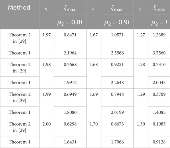
Table 2. Maximum allowable delay upper bound ${\xi }_{\text{max}}$ for various $\varsigma$ and ${\mu }_2$.

Table 3

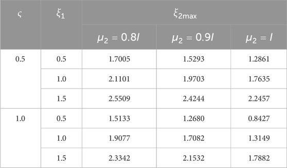
Table 3. Maximum allowable delay upper bound ${\xi }_{2\text{max}}$ for various $\varsigma$, ${\xi }_1$, and ${\mu }_2$ in Theorem 3.

Example 2. Consider MJHNNs Equation 5 and Equation 32 with

$\begin{array}{llllllllll}\hfill & A_1=\left[\begin{array}{cc}\hfill 0.8\hfill & \hfill 0\hfill \\ \hfill 0\hfill & \hfill 1.0\hfill \end{array}\right],\hfill & \hfill & C_1=\left[\begin{array}{cc}\hfill 0.5\hfill & \hfill 0.2\hfill \\ \hfill 0.6\hfill & \hfill 0.3\hfill \end{array}\right],\hfill & \hfill & D_1=\left[\begin{array}{cc}\hfill 0.1\hfill & \hfill 0\hfill \\ \hfill -0.1\hfill & \hfill 0.2\hfill \end{array}\right],\hfill & \hfill & G_1=\left[\begin{array}{cc}\hfill -0.2\hfill & \hfill -0.1\hfill \\ \hfill 0.3\hfill & \hfill 0.1\hfill \end{array}\right],\hfill & \hfill & B_1=\left[\begin{array}{cc}\hfill 0.6\hfill & \hfill 0.3\hfill \\ \hfill 0.2\hfill & \hfill 0.8\hfill \end{array}\right],\hfill \\ \hfill & A_2=\left[\begin{array}{cc}\hfill 1.0\hfill & \hfill 0\hfill \\ \hfill 0\hfill & \hfill 1.2\hfill \end{array}\right],\hfill & \hfill & C_2=\left[\begin{array}{cc}\hfill 0.6\hfill & \hfill 0.3\hfill \\ \hfill 0.7\hfill & \hfill 0.6\hfill \end{array}\right],\hfill & \hfill & D_2=\left[\begin{array}{cc}\hfill 0.2\hfill & \hfill 0.1\hfill \\ \hfill 0.1\hfill & \hfill 0.3\hfill \end{array}\right],\hfill & \hfill & G_2=\left[\begin{array}{cc}\hfill 0.1\hfill & \hfill 0.2\hfill \\ \hfill -0.2\hfill & \hfill 0.3\hfill \end{array}\right],\hfill & \hfill & B_2=\left[\begin{array}{cc}\hfill 0.8\hfill & \hfill 0.5\hfill \\ \hfill 0.6\hfill & \hfill 0.9\hfill \end{array}\right],\hfill \\ \hfill & {\eta }_{11}=-0.2,\hfill & \hfill & {\eta }_{22}=-0.8,\hfill & \hfill & {\mu }_1=-{\mu }_2=-0.5I,\hfill & \hfill & {\lambda }_1=-0.2I,\hfill & \hfill & {\lambda }_2=0.3I.\hfill \end{array}$

Next, we design state estimators to ensure the MSES of FESs with discrete and distributed delays, considering cases of time-invariant and time-variant discrete delays.

Case 1. Time-invariant discrete delay.

For the FES Equation 5, with $\varsigma =1.5$, $\xi =1.0$, and $\epsilon =0.9$, solving the LMIs in Theorem 2 yields the estimator Equation 4 with gain matrices

$K_1=\left[\begin{array}{cc}\hfill 0.6317\hfill & \hfill 0.0146\hfill \\ \hfill 0.1439\hfill & \hfill 0.6857\hfill \end{array}\right],K_2=\left[\begin{array}{cc}\hfill 0.4783\hfill & \hfill 0.2092\hfill \\ \hfill 0.2351\hfill & \hfill 0.5689\hfill \end{array}\right].$

Case 2. Time-variant discrete delay.

For the FES Equation 32, with $\varsigma =1.5$, ${\xi }_1=0.5$, ${\xi }_2=1.5$, and $\epsilon =0.9$, solving the LMIs in Theorem 4 yields the estimator Equation 32 with gain matrices

$K_1=\left[\begin{array}{cc}\hfill 0.6739\hfill & \hfill -0.0045\hfill \\ \hfill 0.1310\hfill & \hfill 0.7854\hfill \end{array}\right],K_2=\left[\begin{array}{cc}\hfill 0.5257\hfill & \hfill 0.1694\hfill \\ \hfill 0.1774\hfill & \hfill 0.6153\hfill \end{array}\right].$

In the simulations, we set $\delta (\vartheta )=0.25\sin \vartheta +0.05\vartheta$, $\phi (\vartheta )=0.5\sin \vartheta$, and

$\vartheta \left(s\right)=\left[\begin{array}{c}\hfill 1\hfill \\ \hfill 0.5\hfill \end{array}\right],\widehat{\vartheta }\left(s\right)=\left[\begin{array}{c}\hfill -1\hfill \\ \hfill 1.5\hfill \end{array}\right],s\in \left[\begin{array}{cc}\hfill -2\hfill & \hfill 0\hfill \end{array}\right].$

The simulations of the state estimators are shown in Figures 1–4. For the MJHNN with time-invariant discrete and distributed delays, Figure 1 shows the state trajectories and their corresponding estimations, while Figure 2 shows the trajectories of the FES. Figures 3, 4 show the corresponding trajectories under time-variant discrete delay scenarios. The proposed state estimator design methods are effective for MJHNNs with discrete and distributed delays in both cases of time-invariant and time-variant discrete delays.

Figure 1

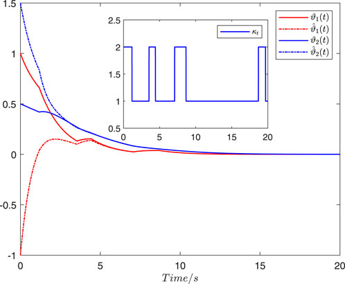
Figure 1. State trajectories ${\vartheta }_1(t)$ and ${\vartheta }_2(t)$, estimations ${\widehat{\vartheta }}_1(t)$ and ${\widehat{\vartheta }}_2(t)$, and Markovian chain ${\kappa }_t$ (Case 1).

Figure 2

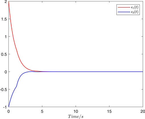
Figure 2. State trajectories of the FES ${ϵ}_1(t)$ and ${ϵ}_2(t)$ (Case 1).

Figure 3

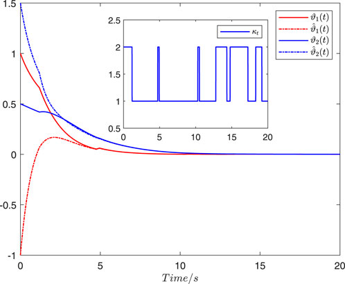
Figure 3. State trajectories ${\vartheta }_1(t)$ and ${\vartheta }_2(t)$, estimations ${\widehat{\vartheta }}_1(t)$ and ${\widehat{\vartheta }}_2(t)$, and Markovian chain ${\kappa }_t$ (Case 2).

Figure 4

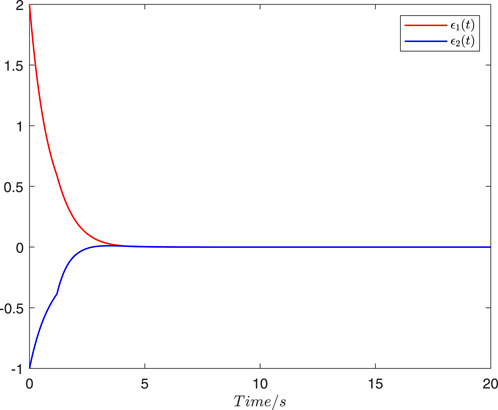
Figure 4. State trajectories of the FES ${ϵ}_1(t)$ and ${ϵ}_2(t)$ (Case 2).

6 Conclusion

This paper has investigated the state estimation for MJHNNs with discrete and distributed delays. Specifically, both time-invariant and time-variant discrete delay cases are considered. Two conditions for the MSES of MJHNNs have been proposed utilizing augmented LKFs, the WBII, the BLI, and the CCI. The LMIs-based design methods for the required estimators have been developed by eliminating nonlinear coupling terms. Lastly, two numerical examples are given to demonstrate the applicability and reduced conservatism of the proposed stability criteria and estimator design methods. Future research could explore further refinement of these analysis and design results, and exporing their extention to more complex neural network models.

Data availability statement

The raw data supporting the conclusion of this article will be made available by the authors, without undue reservation.

Author contributions

LG: Investigation, Methodology, Writing–review and editing. WH: Writing–original draft.

Funding

The author(s) declare that no financial support was received for the research, authorship, and/or publication of this article.

Conflict of interest

The authors declare that the research was conducted in the absence of any commercial or financial relationships that could be construed as a potential conflict of interest.

Publisher’s note

All claims expressed in this article are solely those of the authors and do not necessarily represent those of their affiliated organizations, or those of the publisher, the editors, and the reviewers. Any product that may be evaluated in this article, or claim that may be made by its manufacturer, is not guaranteed or endorsed by the publisher.

References

1. Xiang S, Zhang T, Han Y, Guo X, Zhang Y, Shi Y, et al. Neuromorphic speech recognition with photonic convolutional spiking neural networks. IEEE J Sel Top Quan Electron (2023) 29:1–7. doi:10.1109/JSTQE.2023.3240248

CrossRef Full Text | Google Scholar

2. Cui G, Yang W, Yu J. Neural network-based finite-time adaptive tracking control of nonstrict-feedback nonlinear systems with actuator failures. Inf Sci (2021) 545:298–311. doi:10.1016/j.ins.2020.08.024

CrossRef Full Text | Google Scholar

3. Pan C, Hong Q, Wang X. A novel memristive chaotic neuron circuit and its application in chaotic neural networks for associative memory. IEEE Trans Comput Aided Des Integr Circuits Syst (2021) 40:521–32. doi:10.1109/TCAD.2020.3002568

CrossRef Full Text | Google Scholar

4. Sharma P, Bisht I, Sur A. Wavelength-based attributed deep neural network for underwater image restoration. Acm T Multim Comput (2023) 19:1–23. doi:10.1145/3511021

CrossRef Full Text | Google Scholar

5. Marcus C, Westervelt R. Stability of analog neural networks with delay. Phys Rev A (1989) 39:347–59. doi:10.1103/PhysRevA.39.347

PubMed Abstract | CrossRef Full Text | Google Scholar

6. Gunasekaran N, Thoiyab NM, Zhu Q, Cao J, Muruganantham P. New global asymptotic robust stability of dynamical delayed neural networks via intervalized interconnection matrices. IEEE Trans Cybern (2022) 52:11794–804. doi:10.1109/TCYB.2021.3079423

PubMed Abstract | CrossRef Full Text | Google Scholar

7. Liu M, Jiang H, Hu C, Lu B, Li Z. Novel global asymptotic stability and dissipativity criteria of BAM neural networks with delays. Front Phys (2022) 10:898589. doi:10.3389/fphy.2022.898589

CrossRef Full Text | Google Scholar

8. Chang S, Wang Y, Zhang X, Wang X. A new method to study global exponential stability of inertial neural networks with multiple time-varying transmission delays. Math Comput Simul (2023) 211:329–40. doi:10.1016/j.matcom.2023.04.008

CrossRef Full Text | Google Scholar

9. Tai W, Zhao A, Guo T, Zhou J. Delay-independent and dependent L2-L filter design for time-delay reaction–diffusion switched Hopfield networks. Circ Syst Signal Pr (2023) 42:173–98. doi:10.1007/s00034-022-02125-0

CrossRef Full Text | Google Scholar

10. Zhou J, Ma X, Yan Z, Arik S. Non-fragile output-feedback control for time-delay neural networks with persistent dwell time switching: a system mode and time scheduler dual-dependent design. Neural Netw (2024) 169:733–43. doi:10.1016/j.neunet.2023.11.007

PubMed Abstract | CrossRef Full Text | Google Scholar

11. Rajchakit G, Sriraman R. Robust passivity and stability analysis of uncertain complex-valued impulsive neural networks with time-varying delays. Neural Process Lett (2021) 53:581–606. doi:10.1007/s11063-020-10401-w

CrossRef Full Text | Google Scholar

12. Wang L, He H, Zeng Z. Global synchronization of fuzzy memristive neural networks with discrete and distributed delays. IEEE Trans Fuzzy Syst (2019) 28:2022–34. doi:10.1109/TFUZZ.2019.2930032

CrossRef Full Text | Google Scholar

13. Wang H, Wei G, Wen S, Huang T. Generalized norm for existence, uniqueness and stability of Hopfield neural networks with discrete and distributed delays. Neural Netw (2020) 128:288–93. doi:10.1016/j.neunet.2020.05.014

PubMed Abstract | CrossRef Full Text | Google Scholar

14. Wang G, Ren Y, Huang C. Stabilizing control of Markovian jump systems with sampled switching and state signals and applications. Int J Robust Nonlin (2023) 33:5198–228. doi:10.1002/rnc.6637

CrossRef Full Text | Google Scholar

15. Zhou J, Dong J, Xu S. Asynchronous dissipative control of discrete-time fuzzy Markov jump systems with dynamic state and input quantization. IEEE Trans Fuzzy Syst (2024) 31:3906–20. doi:10.1109/TFUZZ.2023.3271348

CrossRef Full Text | Google Scholar

16. Hu B, Guan ZH, Lewis FL, Chen CP. Adaptive tracking control of cooperative robot manipulators with Markovian switched couplings. IEEE Trans Ind Electron (2020) 68:2427–36. doi:10.1109/TIE.2020.2972451

CrossRef Full Text | Google Scholar

17. Chen G, Xia J, Park JH, Shen H, Zhuang G. Asynchronous sampled-data controller design for switched Markov jump systems and its applications. IEEE Trans Syst Man Cybern: Syst (2022) 53:934–46. doi:10.1109/TSMC.2022.3188612

CrossRef Full Text | Google Scholar

18. Ma X, Dong J, Tai W, Zhou J, Paszke W. Asynchronous event-triggered H control for 2D Markov jump systems subject to networked random packet losses. Commun Nonlinear Sci (2023) 126:107453. doi:10.1016/j.cnsns.2023.107453

CrossRef Full Text | Google Scholar

19. Ali MS, Tajudeen MM, Kwon OM, Priya B, Thakur GK. Security-guaranteed filter design for discrete-time Markovian jump delayed systems subject to deception attacks and sensor saturation. ISA Trans (2024) 144:18–27. doi:10.1016/j.isatra.2023.10.020

PubMed Abstract | CrossRef Full Text | Google Scholar

20. Xia W, Xu S, Lu J, Zhang Z, Chu Y. Reliable filter design for discrete-time neural networks with Markovian jumping parameters and time-varying delay. J Franklin Inst (2020) 357:2892–915. doi:10.1016/j.jfranklin.2020.02.039

CrossRef Full Text | Google Scholar

21. Nagamani G, Soundararajan G, Subramaniam R, Azeem M. Robust extended dissipativity analysis for Markovian jump discrete-time delayed stochastic singular neural networks. Neural Comput Appl (2020) 32:9699–712. doi:10.1007/s00521-019-04497-y

CrossRef Full Text | Google Scholar

22. Yang H, Wang Z, Shen Y, Alsaadi FE, Alsaadi FE. Event-triggered state estimation for Markovian jumping neural networks: on mode-dependent delays and uncertain transition probabilities. Neurocomputing (2021) 424:226–35. doi:10.1016/j.neucom.2020.10.050

CrossRef Full Text | Google Scholar

23. Tao J, Xiao Z, Li Z, Wu J, Lu R, Shi P, et al. Dynamic event-triggered state estimation for Markov jump neural networks with partially unknown probabilities. IEEE Trans Neural Networks Learn Syst (2021) 33:7438–47. doi:10.1109/TNNLS.2021.3085001

CrossRef Full Text | Google Scholar

24. Aravind RV, Balasubramaniam P. Stochastic stability of fractional-order Markovian jumping complex-valued neural networks with time-varying delays. Neurocomputing (2021) 439:122–33. doi:10.1016/j.neucom.2021.01.053

CrossRef Full Text | Google Scholar

25. Yao L, Wang Z, Huang X, Li Y, Ma Q, Shen H. Stochastic sampled-data exponential synchronization of Markovian jump neural networks with time-varying delays. IEEE Trans Neural Networks Learn Syst (2023) 34:909–20. doi:10.1109/TNNLS.2021.3103958

CrossRef Full Text | Google Scholar

26. Tai W, Li X, Zhou J, Arik S. Asynchronous dissipative stabilization for stochastic Markov-switching neural networks with completely-and incompletely-known transition rates. Neural Netw (2023) 161:55–64. doi:10.1016/j.neunet.2023.01.039

PubMed Abstract | CrossRef Full Text | Google Scholar

27. Sathishkumar V, Vadivel R, Cho J, Gunasekaran N. Exploring the finite-time dissipativity of Markovian jump delayed neural networks. Alex Eng J (2023) 79:427–37. doi:10.1016/j.aej.2023.07.073

CrossRef Full Text | Google Scholar

28. Wang T, Zhao S, Zhou W, Yu W. Finite-time state estimation for delayed Hopfield neural networks with Markovian jump. Neurocomputing (2015) 156:193–8. doi:10.1016/j.neucom.2014.12.062

CrossRef Full Text | Google Scholar

29. Chen Y, Zheng WX. Stochastic state estimation for neural networks with distributed delays and Markovian jump. Neural Netw (2012) 25:14–20. doi:10.1016/j.neunet.2011.08.002

PubMed Abstract | CrossRef Full Text | Google Scholar

30. Yao L, Huang X, Wang Z, Liu K. Secure control of Markovian jumping systems under deception attacks: an attack-probability-dependent adaptive event-trigger mechanism. IEEE Trans Control Netw Syst (2023) 10:1818–30. doi:10.1109/TCNS.2023.3269007

CrossRef Full Text | Google Scholar

31. Khalil H. Nonlinear systems. Pearson education. Prentice Hall (2002).

Google Scholar

32. Zheng F, Li X, Du B. Periodic solution problems of neutral-type stochastic neural networks with time-varying delays. Front Phys (2024) 12:1338799. doi:10.3389/fphy.2024.1338799

CrossRef Full Text | Google Scholar

33. Chen Q, Liu X, Wang F. Improved results on L₂-L state estimation for neural networks with time-varying delay. Circ Syst Signal Pr (2022) 41:122–46. doi:10.1007/s00034-021-01799-2

CrossRef Full Text | Google Scholar

34. Qian W, Xing W, Fei S. H state estimation for neural networks with general activation function and mixed time-varying delays. IEEE Trans Neural Networks Learn Syst (2020) 32:3909–18. doi:10.1109/TNNLS.2020.3016120

CrossRef Full Text | Google Scholar

35. Seuret A, Gouaisbaut F. Hierarchy of LMI conditions for the stability analysis of time-delay systems. Syst Control Lett (2015) 81:1–7. doi:10.1016/j.sysconle.2015.03.007

CrossRef Full Text | Google Scholar

36. Zeng HB, He Y, Wu M, She J. New results on stability analysis for systems with discrete distributed delay. Automatica (2015) 60:189–92. doi:10.1016/j.automatica.2015.07.017

CrossRef Full Text | Google Scholar

37. Seuret A, Gouaisbaut F. Wirtinger-based integral inequality: application to time-delay systems. Automatica (2013) 49:2860–6. doi:10.1016/j.automatica.2013.05.030

CrossRef Full Text | Google Scholar

38. Park P, Ko JW, Jeong C. Reciprocally convex approach to stability of systems with time-varying delays. Automatica (2011) 47:235–8. doi:10.1016/j.automatica.2010.10.014

CrossRef Full Text | Google Scholar

39. Liu K, Seuret A, Xia Y. Stability analysis of systems with time-varying delays via the second-order Bessel–Legendre inequality. Automatica (2017) 76:138–42. doi:10.1016/j.automatica.2016.11.001

CrossRef Full Text | Google Scholar

40. Zhou J, Dong J, Xu S, Ahn CK. Input-to-state stabilization for Markov jump systems with dynamic quantization and multimode injection attacks. IEEE Trans Syst Man Cybern: Syst (2024) 54:2517–29. doi:10.1109/TSMC.2023.3344869

CrossRef Full Text | Google Scholar