Surface roughness measurement using microscopic vision and deep learning

Due to the self-affine property of the grinding surface, the sample images with different roughness captured by the micron-scale camera exhibit certain similarities. This similarity affects the prediction accuracy of the deep learning model. In this paper, we propose an illumination method that can mitigate the impact of self-affinity using the two-scale fractal theory as a foundation. This is followed by the establishment of a machine vision detection method that integrates a neural network and correlation function. Initially, a neural network is employed to categorize and forecast the microscopic image of the workpiece surface, thereby determining its roughness category. Subsequently, the corresponding correlation function is determined in accordance with the established roughness category. Finally, the surface roughness of the workpiece was calculated based on the correlation function. The experimental results demonstrate that images obtained using this lighting method exhibit significantly enhanced accuracy in neural network classification. In comparison to traditional lighting methods, the accuracy of this method on the micrometer scale has been found to have significantly increased from approximately 50% to over 95%. Concurrently, the mean squared error (MSE) of the surface roughness calculated by the proposed method does not exceed 0.003, and the mean relative error (MRE) does not exceed 5%. The two-scale fractal geometry offers a novel approach to image processing and machine learning, with significant potential for advancement.

1 Introduction

The grinding surface exhibits a multitude of intricate geometric characteristics [1, 2], however, when observed through the lens of an ordinary camera, the resulting image, while displaying a random texture and weak features, fails to elucidate the distribution trend of surface waviness. A macro scale image for surface roughness was a great start, but to really get to grips with the surface’s geometrical properties, we need to zoom in to the micro scale. This follows the two-scale fractal theory [3–5], which can be applied to various fractal-like patterns [6–8], especially the fractal solitary theory, which was borne by the two-scale fractal concept [9–12]. Surface microstructures exhibit fractal patterns [13–15], and surface roughness on the nanoscale plays a pivotal role in the surface’s properties [16–20]. Consequently, the ordinary camera is unsuitable for precision measurement. The advent of machine vision [21–24] has opened a new avenue for rapid and precise on-line measurement. Deep learning has emerged as a valuable tool for analyzing microscopic vision [25].

Due to the advantages of deep learning [26, 27] in detecting the roughness of the grinding surface, including low cost, high efficiency, non-contact, and so on, much achievement has been obtained. Guo et al [28] used the signal features related to roughness parameters in grinding processing as a dataset, and predicted the roughness parameters of the grinding surface with the help of long short-term memory network (LSTM) network. Yang et al [29] integrated sparrow search algorithm and deep belief network to construct a deep belief network model (SSA-DBN) based on sparrow search algorithm, and demonstrated the excellent performance of this model in predicting the roughness of grinding surface through a series of experiments. Xiao et al. [30] established a CAN-Network (CAN-N) network coupled with deep learning to predict the roughness parameters of grinding surface, which had good prediction accuracy. EL Ghadoui et al [31] used a deep learning method based on the Faster R-CNN architecture to recognize the roughness of the grinding surface, and achieved a high recognition accuracy. Huang et al [32] proposed a feature fusion approach detection for evaluating the roughness of the grinding surface. This method mitigates the interference of machine vision detection due to the problems of blurred feature information and difficulty in recognizing the roughness of the grinding surface. However, the aforementioned studies that generally use macro-scale captured images to construct the dataset, due to the relatively weak and intricate texture features of the grinding surface, make the accuracy of deep learning-based detection of the roughness of the grinding surface to be constrained by the image texture features to a certain extent. El-Ghadoui et al. [31] also analyzed the problem in their study, in which they observed that the surface texture features of machined surfaces fluctuate due to changes in the camera capturing angle. The fluctuations in these surface texture features are attributed to changes in the incident light source caused by changes in camera angles. This phenomenon is particularly evident on ground surfaces with more intricate texture characteristics, where even minor fluctuations in the incident light source can result in significant variations in surface texture.

In contrast to the deep learning self-extracted image features used for roughness classification, the indicator method necessitates the design of image feature indicators through artificial means. However, the correlation model established based on the indicators and roughness can predict the specific roughness parameter values of the grinding surface, thereby conferring a certain degree of interpretability to the image features. For instance, Lu and colleagues [33] proposed establishing an index relationship between surface roughness and gray level covariance matrix (GLCM) and measuring the roughness parameters of the grinding surface by obtaining the laser scatter image. Yi et al. [34] proposed establishing an index relationship between the color index of each pixel in the color image and surface roughness. This relationship would be used to calculate the roughness value by analyzing the change in color information. Zhang et al. [35] proposed establishing an index relationship between the color indices of each pixel of the color image reflected from the machined surface and the roughness value of each pixel based on the change in color information. The degree of red and green blending of two colors in the reflected image of the processed surface is used to establish an index relationship with the roughness, and to initialize the weights of the machine learning model using the migration fuzzy clustering method (KTFCM-NLS).

Given that the imaging method proposed in this paper incorporates height information into the 2D image, a novel indicator relationship must be established. This paper presents a relationship between the average brightness of image pixel points and surface roughness. The derivation of the evaluation mechanism of the indicator covers the following aspects: Firstly, the shape of the wave crest on the grinding surface is fitted to an ellipse based on fractal analysis [36–38], with the validity of the fit being demonstrated through experimentation. Subsequently, the mathematical relationship between the reflected luminance and the incident angle is determined based on the Lambert model [39], with the final step being the mathematical relationship between the height of the wave crest on the grinding surface and the reflected luminance being proven based on the nature of the ellipse. It is important to note that the use of artificially designed feature indicators may result in the omission of certain information [40]. Consequently, this paper proposes a novel approach to roughness visual detection that combines the respective advantages of metrics detection and deep learning. The proposed method firstly classifies the photos of the grinding surface by deep learning in order to determine the roughness category to which the photos belong. Subsequently, an indicator function is constructed for each category according to the classification results. This step transforms the traditional monotonic function-type indicator into a segmented function type, thereby enhancing the indicator function’s fitting ability.

In summary, exploring an illumination method that can eliminate self-affinity is not only important for improving the accuracy of detecting the roughness of grinding surfaces based on deep learning, but also makes the image have certain depth information, which can then be used to calculate the specific value of roughness using the index relationship.

2 Brightness evaluation of grinding surface roughness

The appearance of brightness and waviness are two of the most important criteria for the success of commercial products [41–43]. In this section, we will construct an optical imaging system capable of eliminating interferometric signal, then establish a mathematical model for the grinding surface, and finally establish a correlation between image pixel point brightness and surface roughness.

2.1 Construction of an optical imaging system capable of eliminating self-affine features

Grinding surface images at the micrometer scale can increase the accuracy and enhance the stability of the texture features observed in the images. Nevertheless, only one scale will result in a reduction in the accuracy of the deep learning model in predicting the roughness of the grinding surface due to the effect of the fractal nature of the grinding surface topography.

The fractal nature of the grinding surface topography refers to the fact that the grinding surface maintains an intrinsically similar structure at different observation scales. However, this similarity is approximately valid for a certain range of scales. In engineering, two-scale fractal models were widely used for treating with approximate similarity [44–47].

Observing the surface with only a single scale is always unbelieving [48], two-scale observation is therefore needed. When the observation scale (Field of view range: 30 mm × 16 mm) on a macroscopic scale is magnified 135 times (Field of view range: 4 mm × 2 mm) on a micrometer scale, the deep texture that is difficult to distinguish at the macroscopic scale becomes clearly visible at the micrometer scale. However, the degree of similarity between these micro-texture features and macro-texture features is not fixed, which leads to grinding surfaces with different roughness levels. Although the morphological characteristics exhibit certain differences at the macro scale, they may be highly similar at the micro scale, as illustrated in Figure 1.

Figure 1

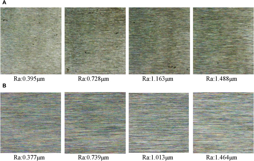
Figure 1. Images acquired at macroscopic and microscopic scales using conventional imaging methods, respectively. (A) Macroscopic scale (Field of view range: 30 mm × 16 mm); (B) Micron scale (Field of view range: 4 mm × 2 mm).

Figure 1 illustrates that, at the macroscopic scale, images with different roughness levels are susceptible to light source noise, yet there are still discernible differences between them. At the micron scale, although the influence of light source noise is reduced, the grinding surface images of different roughness levels may be highly similar. This similarity presents a challenge to deep learning-based machine vision methods, resulting in a decrease in the prediction accuracy of the grinding surface roughness at the microscopic scale.

In order to eliminate the fractal interference to visual detection as much as possible, the position of the light source is changed. In this method, a strip light source is placed in close proximity to the grinding surface, and the position of the light source and the imaging position are fixed. As illustrated in Figure 2, $\overrightarrow{n}$ represents the plane surface normal vector, $\overrightarrow{h}$ denotes the rough surface normal vector, $\overrightarrow{\mu }$ signifies the tangent of the rough surface, ${\theta }_i^{origin}$ is the angle between the incident light and the surface normal of the plane, ${\theta }_i$ is the angle between the incident light direction and the rough surface normal, and ${\theta }_o$ is the angle between the reflected light and the rough surface normal. Due to the distinctive topography of the grinding surface, comprising both high and low peaks, the varying wave peaks will result in occlusion. Only those surface wave peaks in a specific incidence angle range $\left({\theta }_{i\min },{\theta }_{i\max }\right)$ and height range $\left(h_{\min },h_{\max }\right)$ will reflect light at the imaging position. Consequently, the image acquired at the microscopic scale contains height information, which serves to eliminate the influence of the fractal-like surface on the imaging image. Figure 3 illustrates the topography image of the grinding surface acquired by the proposed optical imaging method at the microscopic scale.

Figure 2

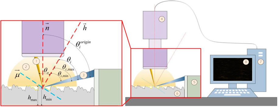
Figure 2. The proposed optical imaging method. 1) All possible specular reflections at the point; 2) All possible diffuse rays at the point; 3) All possible incident rays at the point; 4) Industrial microscope; 5) Strip light source; 6) Sample; 7) Computer; 8) Collected results.

Figure 3

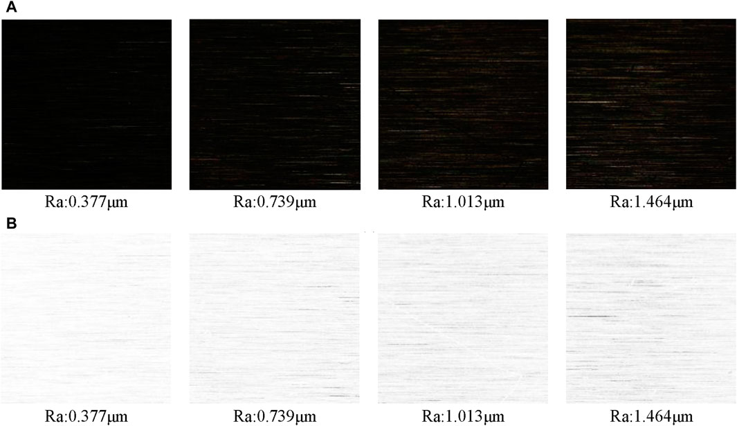
Figure 3. Images were acquired at the micron scale (Field of view range: 4 mm × 2 mm) using the proposed method (A) Real images; (B) The inverse value of the gray value of the real image.

In order to gain a deeper understanding of the image height information obtained by the aforementioned method, and thus elucidate the mechanism of brightness evaluation of grinding surface roughness, this paper will commence the construction of a mathematical model for the grinding surface topography and a surface reflection model. This will be followed by a mathematical derivation to prove that there is a certain relationship between surface height and image brightness. This will lay the foundation for subsequent visual inspection research.

2.2 Mathematical modeling of grinding surface

The grinding surface exhibits similarity property, that is the image on a macro scale is similar to that on a micron scale. In order to construct a grinding surface model that can eliminate fractal interference and highlight the main wave peak topography, this paper proposes an ellipse based on the same major and minor axes to fit the grinding surface topography features. The schematic diagram of the model is presented in Figure 4. When the surface is smooth, as illustrated in Figure 4A, the angle between the incident light and the plane surface normal $\overrightarrow{n}$ is designated as ${\theta }_i^{origin}$. When the surface becomes rough in order to form a grinding surface, the angle between the incident light and the rough surface normal $\overrightarrow{h}$ is expressed as ${\theta }_i$. The wave peak of a single rough surface is shown in Figure 4B. The subsequent step involves fitting the rough crest to an ellipse shape that is raised up by the horizontal face, as illustrated in Figure 4C. In this model, a higher crest corresponds to a larger upward bulge of the ellipse. In this manner, the fitting can negate the impact of wave peaks with self-affine characteristics, thereby reflecting the incidence angle of the primary wave peak.

Figure 4

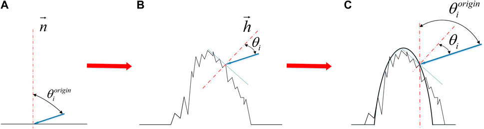
Figure 4. Principle of the proposed model for grinding surface topography. (A) Smooth initial surface; (B) Rough surface after grinding processing; (C) Rough surface after peak fitting.

In order to demonstrate the rationality of this method, this paper initially identified the self-affine points in the two-dimensional point cloud data of the transverse section of the grinding surface obtained by BRUKER Contour X-200 white light interferometer through fractal analysis [36], and then deleted them in order to retain the highest value point in the self-affine point group, as illustrated in Figure 5. Subsequently, the point cloud was clustered using the K-means algorithm [49] in order to ascertain the height of each wave peak. Finally, each cluster was fitted to an ellipse shape with the same major and minor axes by means of the ellipse fitting algorithm. As illustrated in Figure 6, the greater the height of the wave peak, the closer the ellipse’s center was to the peak.

Figure 5

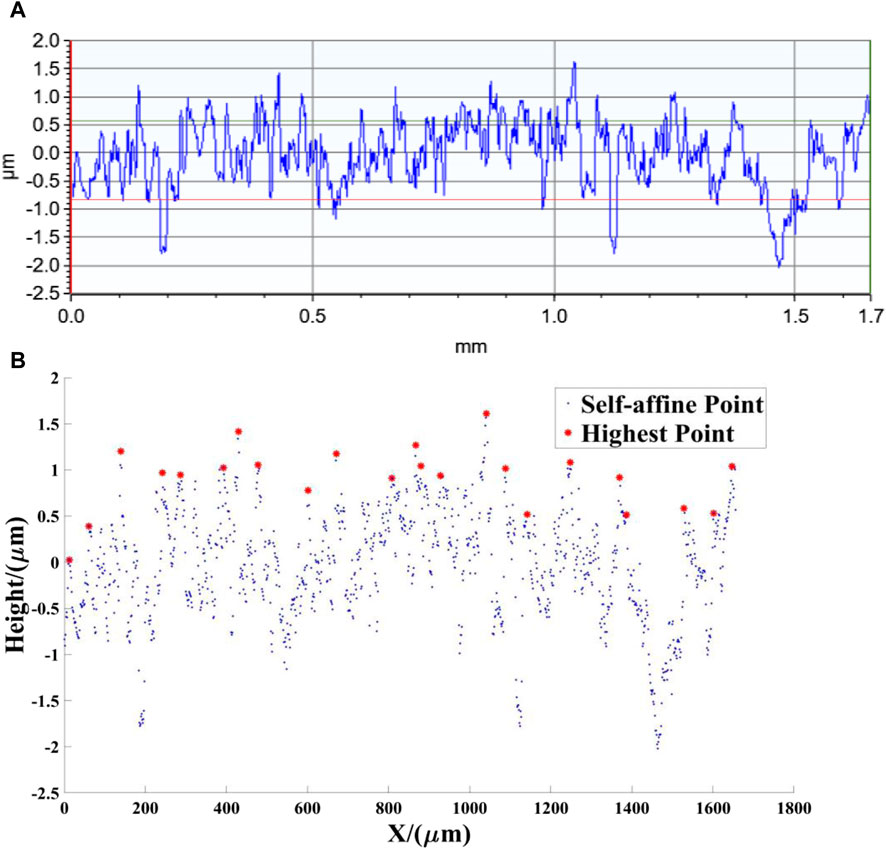
Figure 5. The highest value points among the self-affine points. (A) The measured 2D point cloud data of the transverse section of the grinding workpiece Ra = 0.447 μm; (B) Identification of the highest point in the self-affine point cloud.

Figure 6

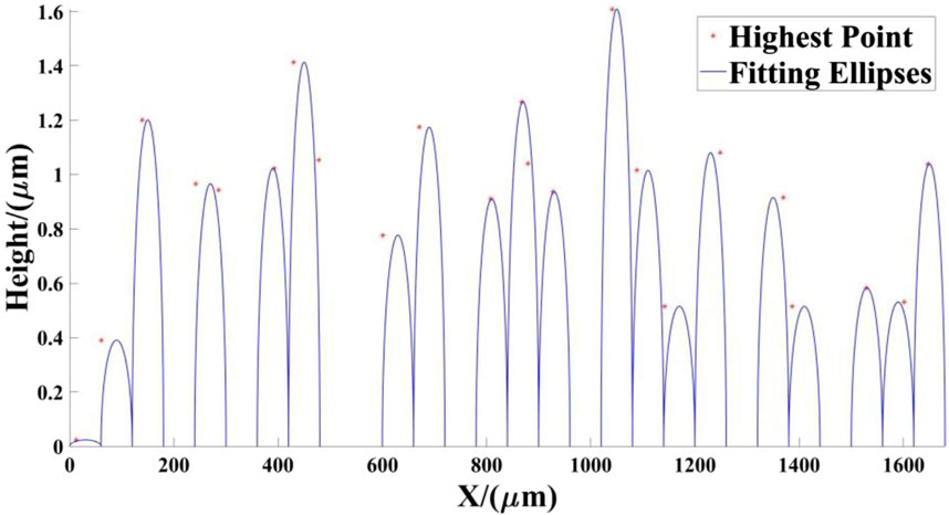
Figure 6. The ellipse model of grinding surface with the long axis of 30 μm and the short axis of 1.0394 μm.

After fitting and analyzing the grinding surfaces with different roughness parameters, the errors of the aforementioned mathematical model for various roughness surfaces are obtained in this paper, and the detailed data are shown in Table 1. In this table, MRE represents the average relative error between the crest point and the fitted ellipse. As can be observed in Table 1, the average relative error of the proposed mathematical model does not exceed 30%. This result indicates that the model has some validity.

Table 1

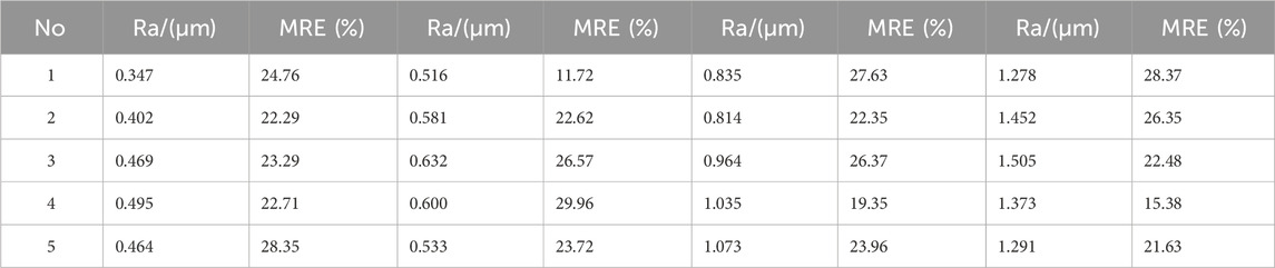
Table 1. Surface fitting errors for different roughness parameters.

2.3 Correlation between image pixel point brightness and surface roughness

In order to accurately simulate the change of the reflected light intensity with the roughness of the grinding surface, the Lambert illumination model [50] is selected to construct the surface reflection model in this paper. The Lambert model is a commonly used optical reflection model that is particularly suited to simulating the diffuse reflection effect of an object’s surface, thereby enabling the accurate reflection of the influence of varying roughness on the reflected light intensity. In the Lambert model, the reflected light intensity at a given point on the surface is expressed as Eq. 1:

$I=I_i\ast k_d\ast \cos \left({\theta }_i\right)(1)$

Here, $I_i$ represents the incident light intensity, $k_d$ represents the diffuse reflection coefficient, and ${\theta }_i$ represents the Angle between the incident light and the surface normal.

In the Lambert model, the intensity of the reflected light is directly affected by the incidence angle, while the magnitude of the incidence angle depends on the distribution of the surface normal. Moreover, the shape of the wave peaks on the grinding surface determines the specific distribution of these normal. Based on the illumination method proposed in this paper and the grinding surface fitting model, further assumptions are made: 1) Due to the small imaging area in this paper, at the micrometer level, it can be assumed that the illumination intensity of the incident light and the incident angle on the horizontal plane are constant. This implies that the light source is assumed to be parallel light. 2) As a result of the topography fitting model eliminating smaller self-affine peaks, the height difference between retained peaks is limited to the micron level. Therefore, it is reasonable to assume that there is no mutual occlusion between the wave peaks. Subsequently, the relationship between the reflected light intensity of a single wave peak and the height of the wave peak is derived as follows.

As shown in Figure 7, when a single parallel ray hits the plane, the angle between its incident ray and the plane normal is ${\theta }_{origin}$, and the incidence angle of parallel lights is unchanged. When the plane becomes an elliptic crest, the angle between its incident ray and the normal of the elliptic surface is ${\theta }_i$. The angle between the surface normal of the ellipse and the Y-axis is $\phi$, which can be expressed as Eq. 2.

${\phi }_i={\theta }_{origin}-{\theta }_i(2)$

Figure 7

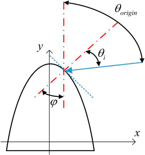
Figure 7. Incidence angles in the fitted model.

In Section 2.2, it is introduced that this article employs the ellipse fitting algorithm to fit the peaks. The ellipses fitted by this fitting method are typically represented in the form of standard ellipse equations. In this context, this article employs the standard equation of an ellipse centered on the y-axis as a case study to illustrate the mathematical relationship between the reflected light intensity of a single ray and the relative position of the wave peak.

$\frac{y^2}{a^2}+\frac{x^2}{b^2}=1(3)$

Let $P\left(x_0,y_0\right)$ be a point on the elliptic sphere and the angle between its normal and the X-axis be $90°-{\phi }_i$, then the slope of the normal is $k=-\tan \left(90°-{\phi }_i\right)$ and the slope of the tangent is $-1/k=\tan \left({\phi }_i\right)$.

According to Eq. 3, we have

$y^{\prime }\left(x_0\right)=-\frac{b^2{x}_0}{a^2{y}_0}=\tan \left({\phi }_i\right)(4)$

Additionally, we have

$\frac{y_0^2}{a^2}+\frac{x_0^2}{b^2}=1\left(x_0\ge 0,y_0\ge 0\right)(5)$

Solving the above equations simultaneous, we have

$y_0=\frac{a{b}^3}{\sqrt{a^6\tan \left({\phi }_i\right)+b^6}}(6)$

When multiple parallel lights are incident, the total reflected light intensity of the wave peak is the sum of the reflected intensity of all rays illuminating on the wave peak. The height difference between different peaks can be expressed as follows.

$\Delta y={\displaystyle \sum _{i=1}^N}\frac{a{b}^3}{\sqrt{a^6\tan \left({\theta }_{origin}-\arccos \left(\frac{I}{k_d{I}_i}\right)\right)+b^6}}-{\displaystyle \sum _{i=1}^{N-\Delta }}\frac{a{b}^3}{\sqrt{a^6\tan \left({\theta }_{origin}-\arccos \left(\frac{I}{k_d{I}_i}\right)\right)+b^6}}(7)$

where $\Delta$ means that $\Delta$ bars are not illuminated on this wave peak due to the height difference. Since a higher wave peak has more incident light, the intensity of the reflected light is also greater, as shown in Figure 8.

Figure 8

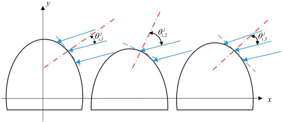
Figure 8. Multiple parallel lights.

The above derivation (Eqs 4–7) demonstrates a correlation between pixel brightness and surface height in the imaging method. Furthermore, the relative position relationship between the surface crest height can be calculated by the pixel brightness, which provides a foundation for the subsequent detection method.

3 Experimental verification

3.1 Flowchart and experimental design

Due to the random texture characteristics of the grinding surface, the shape of the fit ellipse is changeable, and the occlusion ratio between different wave peaks is not fixed. The direct application of the aforementioned derivation to the calculation of the height of each point on the surface will inevitably result in the generation of erroneous data. The surface roughness parameter Ra is an average evaluation index. Consequently, the error can be reduced by the average method, which involves establishing the average brightness value of the image pixel and the surface roughness parameter.

However, due to the change in surface roughness, the diffuse reflection coefficient and specular reflection coefficient of the grinding surface of the same material will change, which will further affect the image pixel brightness. Consequently, establishing a direct correlation between the image pixel brightness and the surface roughness parameter Ra will inevitably result in significant inaccuracies. To address this issue, this paper proposes a method that combines a neural network with an indicator. Firstly, the roughness level of the image is determined by a neural network, and then the specific values of the roughness parameters are predicted based on the indicator relationship functions of each roughness level. The overall method is shown in Figure 9.

Figure 9

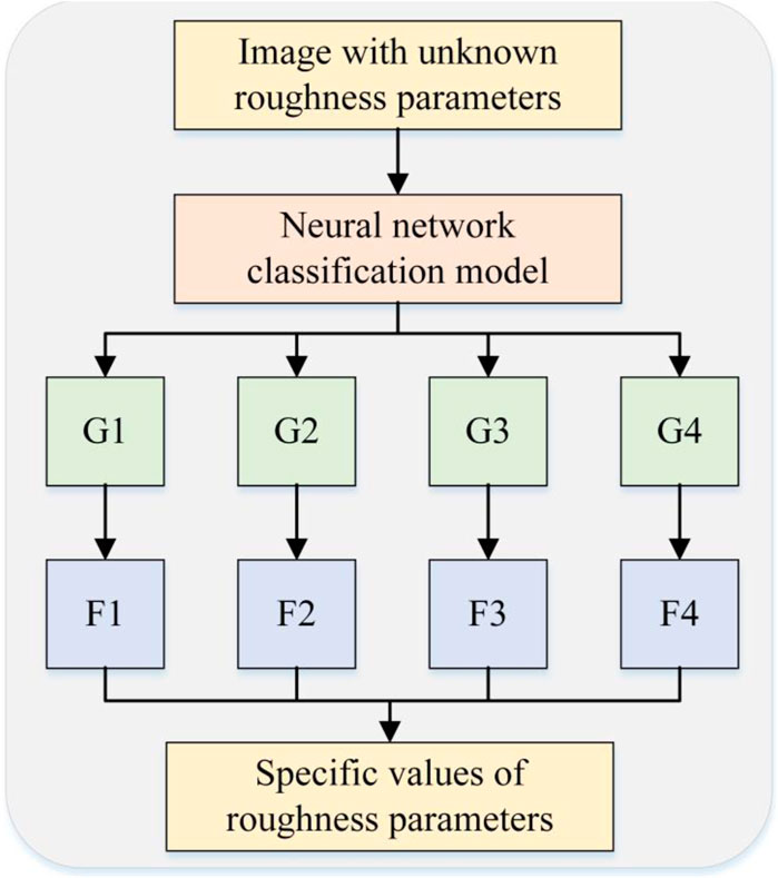
Figure 9. Flow Chart. G1, G2, G3, G4 represent the level of roughness, F1, F2, F3, F4 represent the index function fitted according to the workpiece with different roughness levels.

In order to verify the effectiveness of the proposed method, this paper conducted experimental designs from two aspects: neural network classification and the prediction of specific values for indicators.

With regard to neural network classification, this article refers to the traditional macroscopic vision-based neural network prediction method for grinding surface roughness parameters, as described in [29–32], and the classification accuracy of the aforementioned methods exceeds 90%. In order to gain a deeper understanding of the fractal characteristics of grinding surface morphology and their impact on neural network classification models at the micro scale, the following steps were taken in this paper: Firstly, the reference method [32] conducted classification experiments at the macro scale, with the dataset denoted as D1. Subsequently, this article conducted a replication of the traditional classification experiments at the microscale using the same instruments and equipment, with the dataset denoted as D2. Finally, the proposed method will be applied to the same instrument and equipment for classification experiments at the microscopic scale, with the dataset denoted as D3.

In terms of predicting the specific values of roughness indicators, this article fits the indicator function relationship of different roughness levels by statistically analyzing the correspondence between roughness parameters and image brightness under the proposed method. Once the neural network has predicted the roughness level of an image with unknown roughness, this paper inputs the level into the corresponding index function in order to calculate the specific roughness value. A comparison of the calculated value with the measured value has demonstrated the rationality and accuracy of the method proposed in this paper.

3.2 Preparation of samples

The sample under examination was produced using the M7130 (as shown in Figure 10A) precision horizontal axis grinder, and the workpiece material is 45# steel, a common engineering material. In order to ensure the rationality and scientific nature of the experiment, the commonly used processing parameters are selected in this paper, as shown in Table 2. These include the grinding wheel particle size number, grinding wheel speed, grinding depth, axial feed parameters and transverse feed speed. The specific parameters are presented in tabular form.

Figure 10

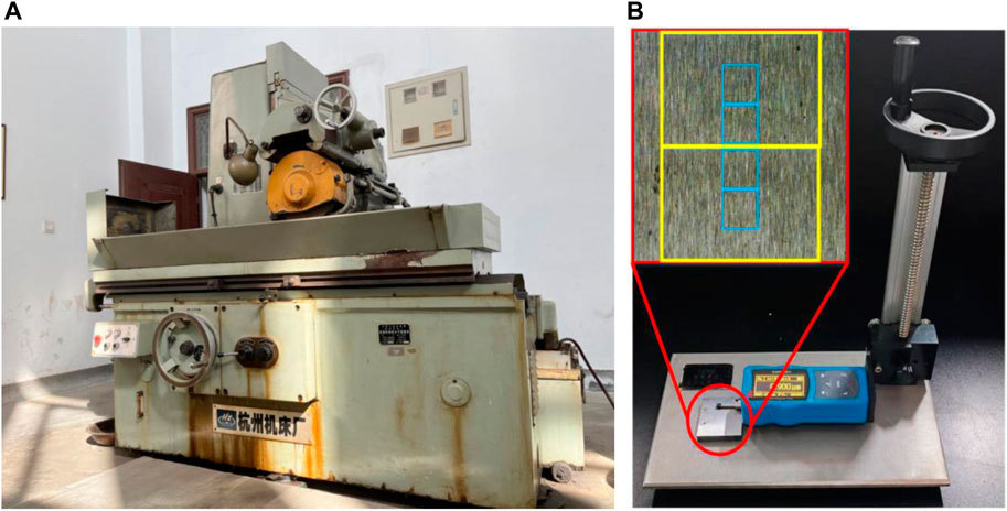
Figure 10. Processing equipment and measuring equipment (A) ordinary horizontal axis moment table surface grinder M7150H (B) surface roughness tester TA260.

Table 2

Table 2. Working conditions.

A total of 80 experimental sample blocks were obtained through processing. In dataset D1, each sample is divided into two detection areas in a manner that is uniform across the entire set, as illustrated by the yellow box in Figure 10B. In datasets D2 and D3, each sample is divided into four detection areas in a manner that is uniform across the entire set, as illustrated by the blue box in Figure 10B. In this study, the surface roughness tester TA260 was employed to conduct five repeated measurements of the roughness parameter Ra in each region. The average of these five measurements was then taken as the roughness parameter value for the region. The overall range of the roughness parameter Ra distribution of the sample is (0.3 μm, 1.6 μm). Subsequently, this paper further subdivides the roughness interval into four categories based on the ISO 1302 roughness grade standard. The four categories are as follows: The range of roughness values (0.3 μm, 0.5 μm) is designated as G1, (0.5 μm, 0.8 μm) as G2, (0.8 μm, 1.2 μm) as G3, and (1.2 μm, 1.6 μm) as G4. Due to the non-uniform distribution of grinding surface roughness, the number of detection regions conforming to each classification interval is also non-uniform. The number of detection regions in each classification interval is provided in Tables 3, 4.

Table 3

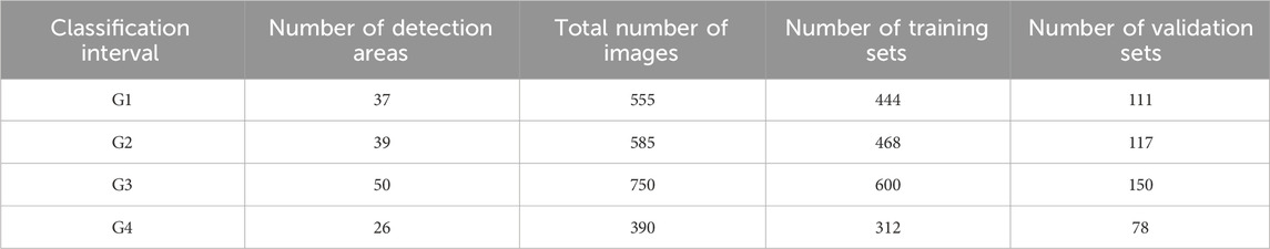
Table 3. Composition of dataset D1.

Table 4

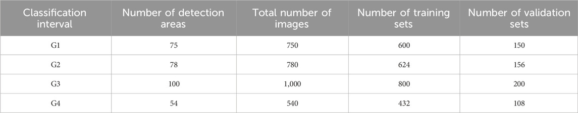
Table 4. Composition of dataset D2 and D3.

3.3 Imaging system and data acquisition

Building upon the theoretical framework presented in the preceding section, an optical imaging system is constructed as depicted in Figure 11. Following the construction of the imaging system, this article selected the GP-660V industrial microscope (resolution: 1920 × 1,080) and equipped it with a 2BRD6030 white light strip light source (color temperature range: 6,500 K–7500 K) and an AR67 white light ring light source (color temperature range: 3,300 K–12,000 K). Subsequently, this article employed both traditional and novel methodologies to capture images of the sample detection area at the millimeter scale (field of view range: The dimensions of the sample detection area were 30 mm × 16 mm, with a working distance of 115 mm and a depth of field of 14 mm. At the micrometer scale, the field of view range was 4 mm × 2 mm, the working distance was 85 mm, and the depth of field was 2 mm. Specifically, at the micrometer scale, this article employed two distinct methods for image acquisition, which were subsequently subjected to comparative analysis.

Figure 11

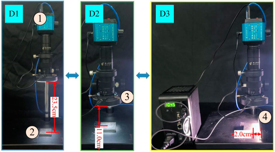
Figure 11. Imaging systems corresponding to different datasets. 1) Industrial microscope; 2) Workpiece; 3) Circular light source; 4) Bar light source.

The study randomly selected 10 images from each of the 10 detection areas. In order to expand the data set, techniques such as rotation and cropping were employed for the D1 dataset. This ensured that each detection area contained 15 images. For datasets D2 and D3, this article did not implement data augmentation operations to ensure that the sample size in the D1, D2, and D3 datasets is as similar as possible. Once all image processing has been completed, the images are uniformly adjusted to a size of 224 × 224 pixels for subsequent analysis. Subsequently, 80% of the images in each classification interval were randomly selected as the training set, while the remaining images were used as the test set. The number of images in the test set and the training set is presented in Tables 3, 4. It is important to note that, in this paper, the roughness level division is carried out prior to image acquisition. Consequently, in the construction of the data set, whether using the traditional method or the novel method proposed in this paper, the data structure of the two methods is identical. This step ensures the consistency and comparability of data during subsequent image analysis and processing.

3.4 Correlation between image pixel brightness and surface roughness

In the experimental section of this article, we randomly selected 40 detection regions from each of the four classification intervals (G1, G2, G3, G4) of dataset D3 for correlation analysis. Based on these regions, we constructed indicator functions. As the number of detection regions in each classification interval of dataset D3 exceeds 40, an additional 5 regions were selected for inclusion in the validation set, which were not used in the construction of the indicator functions. The validation set was specifically designed to test and verify the accuracy of the constructed indicators. The Figure 12 depicts the fitting curves of roughness and brightness for each classification interval.

Figure 12

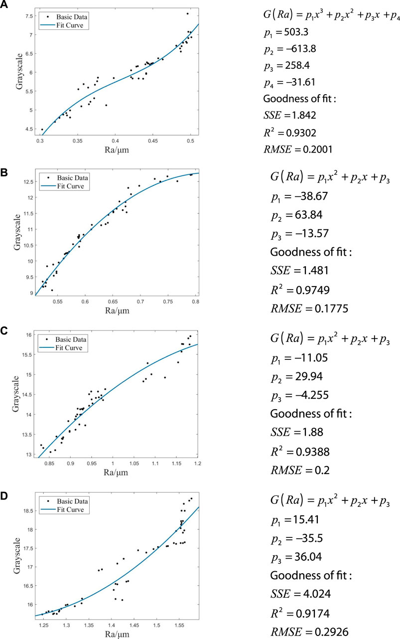
Figure 12. Correlation functions for each classification interval. Correlation functions for the G1 interval (A), the G2 interval (B), the G3 interval (C) and the G4 interval (D).

As illustrated in Figure 12, there is a clear and direct correlation between the roughness and the average brightness of image pixels. In these four correlation functions, the average brightness of image pixels increases with an increase in the roughness parameter.

4 Experiment and result analysis

4.1 Classification based on neural network models

The classification experiment in this paper uses two different sources of experimental data sets, one data set is the grinding surface images at microscopic scale captured by the traditional illumination method, and the other is the grinding surface images acquired at the same scale by the proposed method. In order to make a comprehensive comparison, this paper selects four commonly used classification networks to perform classification experiments on two datasets, including convolutional neural network models: ConvNeXt V2, ResNet 101, lightweight neural network: MobileNet V3, ShufflNet V2. The experimental results are as follows.

Figures 13A–F and Table 5 depicts the outcomes of the training process for each model across distinct datasets. The results demonstrate that, when employing traditional methods and utilising the imaging instrument described in this article, the classification accuracy of the neural network can exceed 90%. When the range of image acquisition is reduced, the accuracy of traditional lighting methods is constrained, with a maximum accuracy of only 52.52%. In contrast, the datasets constructed by the proposed illumination method demonstrate significant advantages, with the highest accuracy of 99.58%. The discrepancy in outcomes can be attributed to the fact that traditional methods solely enhance images by amplifying texture features, which in turn exacerbates self-affine texture noise, thereby negatively impacting the prediction accuracy of deep learning models. Conversely, the proposed illumination method effectively eliminates the interference of self-affine texture features on the topography of the 2D image of the grinding surface. The experimental results presented in this series demonstrate the effectiveness and superiority of the illumination method proposed in this paper.

Figure 13

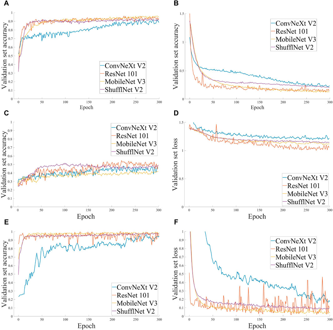
Figure 13. Accuracy and Loss curves for each model using different datasets (A) Accuracy curve for D1 (B) Loss curve for D1 (C) Accuracy curve for D2 (D) Loss curve for D2 (E) Accuracy curve for D3 (F) Loss curve for D3.

Table 5

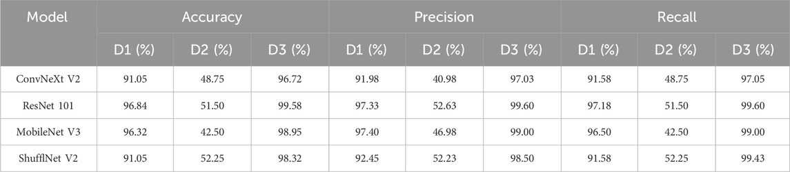
Table 5. Evaluation index parameters of each model.

Furthermore, an examination of the accuracy and loss curves between convolutional neural network models and lightweight neural network models in deep learning models reveals that, despite the superior accuracy of convolutional neural network models (ConvNeXt V2, ResNet 101) (99.58%), the loss curves (depicted by the blue and orange curves in Figure 13D) exhibit considerable fluctuations. In other words, even after the overall convergence of the loss curve, the discrepancy in loss values will remain above 0.2. In contrast, the lightweight neural network model can not only achieve a high accuracy (stable above 98%), but also its prediction results are more stable than those of convolutional neural networks. This phenomenon can be attributed to the relatively modest size of the current dataset produced in this study. At this scale, lightweight neural networks are able to demonstrate their full potential, whereas convolutional neural networks are constrained by the limitations of the data volume. Consequently, at this data scale, the lightweight neural network model exhibits enhanced stability and practicality.

Figure 14 depicts the confusion matrices of each model on distinct test sets. It is evident that there is confusion among the morphological features of images with disparate roughness parameters captured at the micron scale using the traditional illumination method. In particular, the confusion between G1 (0.3 μm, 0.5 μm) and G2 (0.5 μm, 0.8 μm) and between G3 (0.8 μm, 1.2 μm) and G4 (1.2 μm, 1.6 μm) is pronounced. The data indicates that the similarity ratio of the self-affine texture of the grinding surface exhibits fluctuations within the ranges of roughness parameters (0.3 μm, 0.8 μm) and texture characteristics (0.8 μm, 1.6 μm).

Figure 14

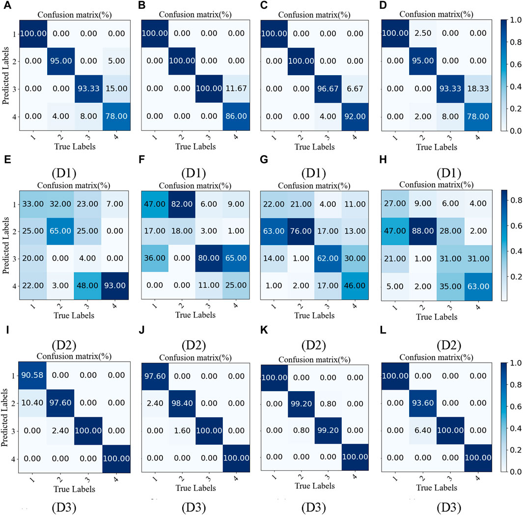
Figure 14. Confusion matrices for each model on different test sets. (A) ConvNeXt V2 (B) MobileNet V3 (C) ResNet 101 (D) ShufflNet V2 (E) ConvNeXt V2 (F) MobileNet V3 (G) ResNet 101 (H) ShufflNet V2 (I) ConvNeXt V2 (J) MobileNet V3 (K) ResNet 101 (L) ShufflNet V2.

4.2 Prediction of roughness parameter

Following the processing of the deep learning classification model, the image of the test area was successfully classified, and its roughness level and the corresponding index function were determined. In order to verify the effectiveness of the index, this paper selects five detection areas in each roughness level of the test set as the validation set of the test index. The specific values of the roughness parameters of the sample block to be tested are then predicted through the pictures of the sample block according to the corresponding index functions. The experimental results are presented in Table 6.

Table 6

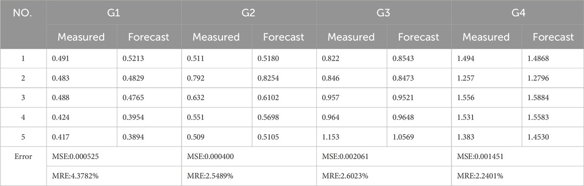
Table 6. Measured results (Ra:μm).

Table 6 illustrates that the average relative error between the predicted value and the measured value of the indicator function remains below 5%, thereby demonstrating that the proposed indicator relationship exhibits satisfactory detection performance. Nevertheless, it is evident that the precision of the index function prediction exhibits fluctuations within the narrow range of roughness levels, spanning from 0.3 μm to 0.5 μm. In particular, there is an instance where an image originally belonging to roughness level G1 was incorrectly predicted to be an image of roughness level G2. This phenomenon indicates that the self-affine texture noise is not readily eliminated by our method at the micron scale due to the fluctuation of the self-affine texture similarity ratio in the region with relatively weak texture features. Further research is necessary to investigate this issue.

5 Conclusion

This paper presents a visual inspection method that can eliminate the influence of self-affine grinding surfaces. The method is constructed by improving the illumination method and combining the neural network with the specific index evaluation method. Firstly, the neural network model is employed to categorize the grinding surface, and subsequently, the specific value of the roughness is calculated in accordance with the index function. Experimental data shows that the imaging method proposed in this article can achieve a classification accuracy of 99.58% for neural networks, and the average relative error of the specific value of the roughness predicted by the index is less than 5%. The experimental results demonstrate the effectiveness of the proposed method. The results of the experiments allow the following conclusions to be drawn:

1. The accuracy of neural network classification is negatively impacted when the image capture scale is reduced, particularly when traditional lighting methods are employed. However, the lighting method proposed in this article is an effective solution to this problem and improves classification accuracy.

2. Once the self-affine texture noise has been eliminated from the 2-D topography image of the grinding surface at the micron scale, the average brightness of the image is larger and the roughness of the image is also larger.

3. The similarity ratio of the self-affine texture of the grinding surface exhibits fluctuations within the ranges of roughness parameters (0.3 μm, 0.8 μm) and texture characteristics (0.8 μm, 1.6 μm).

4. In the region with relatively weak texture features, the fluctuation of the self-affine texture similarity ratio precludes the complete elimination of self-affine texture noise by changing the illumination method at the micron scale.

In the context of the proposed illumination method for surface reconstruction, two approximation assumptions may potentially lead to errors. To enhance the precision of the study, future research may wish to examine the change ratio of the fitted ellipse shape under varying roughness parameters in greater depth, as well as the specific occlusion ratio between different wave peaks. Concurrently, researchers may endeavor to integrate binocular reconstruction technology with the illumination method proposed in this paper, thereby investigating the broader potential applications of this fusion technology in the domain of surface reconstruction. Additionally the fractional calculus [51] and the optimization-based detection system [52, 53] and the variational iteration method [54] might be also applied for the fractal image process. Furthermore the deep learning technology can be also applied to Micro-electromechanical Systems [55, 56, 57].

Data availability statement

The data analyzed in this study is subject to the following licenses/restrictions: The author is not authorized to disclose the dataset. Requests to access these datasets should be directed to CS 1113019533@qq.com.

Author contributions

CS: Writing–original draft, Conceptualization, Data curation, Visualization. ZL: Formal Analysis, Software, Writing–original draft. KG: Methodology, Project administration, Resources, Writing–original draft. HY: Investigation, Resources, Supervision, Validation, Writing–review and editing.

Funding

The author(s) declare that financial support was received for the research, authorship, and/or publication of this article. The National Natural Science Foundation of China (Grant No. 52065016); Taif University, Saudi Arabia, for supporting this work through project number (TU-DSPP-2024-45).

Acknowledgments

The authors extend their appreciation to the National Natural Science Foundation of China (Grant No. 52065016) and Taif University, Saudi Arabia, for supporting this work through project number (TU-DSPP-2024-45).

Conflict of interest

The authors declare that the research was conducted in the absence of any commercial or financial relationships that could be construed as a potential conflict of interest.

Publisher’s note

All claims expressed in this article are solely those of the authors and do not necessarily represent those of their affiliated organizations, or those of the publisher, the editors and the reviewers. Any product that may be evaluated in this article, or claim that may be made by its manufacturer, is not guaranteed or endorsed by the publisher.

References

1. Pan Y, Zhao Q, Guo B, Chen B, Wang J, Wu X. An investigation of the surface waviness features of ground surface in parallel grinding process. Int J Mech Sci (2020) 170:105351. doi:10.1016/j.ijmecsci.2019.105351

CrossRef Full Text | Google Scholar

2. Wu M, Guo B, Zhao Q, He P. Precision grinding of a microstructured surface on hard and brittle materials by a microstructured coarse-grained diamond grinding wheel. Ceram Int (2018) 44(7):8026–34. doi:10.1016/j.ceramint.2018.01.243

CrossRef Full Text | Google Scholar

3. Aln QT, He JH. On two-scale dimension and its applications. Therm Sci (2019) 23(3):1707–12.

CrossRef Full Text | Google Scholar

4. He JH, Ain QT. New promises and future challenges of fractal calculus: from two-scale thermodynamics to fractal variational principle. Therm Sci (2020) 24(2):659–81. doi:10.2298/tsci200127065h

CrossRef Full Text | Google Scholar

5. Ain QT, He JH, Qiang XL, Kou Z. The two-scale fractal dimension: a unifying perspective to metabolic law. Fractals (2024) 32(01):2450016. doi:10.1142/s0218348x24500166

CrossRef Full Text | Google Scholar

6. Sun JS. Variational principle for fractal high-order long water-wave equation. Therm Sci (2023) 27(3A):1899–905. doi:10.2298/tsci2303899s

CrossRef Full Text | Google Scholar

7. Sun JS. Fractal modification of Schrodinger equation and its fractal variational principle. Therm Sci (2023) 27(3A):2029–37. doi:10.2298/tsci2303029s

CrossRef Full Text | Google Scholar

8. Jiao ML, He JH, He CH, et al. Variational principle for Schrödinger-KdV system with the M-fractional derivatives. J Comput Appl Mech (2024) 55(2):235–41. doi:10.22059/jcamech.2024.374235.1012

CrossRef Full Text | Google Scholar

9. He JH, Hou WF, He CH, Saeed T, Hayat T. Variational approach to fractal solitary waves. Fractals (2021) 29(07):2150199. doi:10.1142/s0218348x21501991

CrossRef Full Text | Google Scholar

10. He JH, Qie N, He CH. Solitary waves travelling along an unsmooth boundary. Results Phys (2021) 24:104104. doi:10.1016/j.rinp.2021.104104

CrossRef Full Text | Google Scholar

11. Lv GJ, Tian D, Xiao M, et al. Shock-like waves with finite amplitudes. J Comput Appl Mech (2024) 55(1):1–7. doi:10.22059/JCAMECH.2024.372024.958

CrossRef Full Text | Google Scholar

12. Wu Y, He JH. Variational principle for the Kaup-Newell system. J Comput Appl Mech (2023) 54(3):405–9. doi:10.22059/JCAMECH.2023.365116.875

CrossRef Full Text | Google Scholar

13. Babič M, Marinkovic D, Bonfanti M, Calì M. Complexity modeling of steel-laser-hardened surface microstructures. Appl Sci (2022) 12:2458. doi:10.3390/app12052458

CrossRef Full Text | Google Scholar

14. Babič M, Marinković D. A new approach to determining the network fractality with application to robot-laser-hardened surfaces of materials. Fractal and Fractional (2023) 7(10):710. doi:10.3390/fractalfract7100710

CrossRef Full Text | Google Scholar

15. Babič M, Marinković D, Kovačič M, Šter B, Calì M. A new method of quantifying the complexity of fractal networks. Fractal and Fractional (2022) 6:282. doi:10.3390/fractalfract6060282

CrossRef Full Text | Google Scholar

16. Ghamari F, Raoufi D, Arjomandi J, Nematollahi D Surface fractality and crystallographic texture properties of mixed and mono metallic MOFs as a new concept for energy storage devices. Colloids Surf A (2023) 656A:130450. doi:10.1016/j.colsurfa.2022.130450

CrossRef Full Text | Google Scholar

17. Packham DE. Surface energy, surface topography and adhesion. Int J Adhes Adhes (2003) 23(6):437–48. doi:10.1016/s0143-7496(03)00068-x

CrossRef Full Text | Google Scholar

18. Lan Z, Ma X, Wang S, et al. Effects of surface free energy and nanostructures on dropwise condensation. Chem Eng J (2010) 156(3):546–52.

Google Scholar

19. Liovic D, Franulovic M, Eakins D, et al. Surface roughness of Ti6Al4V alloy produced by laser powder bed fusion. Facta Universitatis Ser Mech Eng (2024) 22(1):63–76.

Google Scholar

20. Zuo YT. Variational principle for a fractal lubrication problem. Fractals (2024):2450080. doi:10.1142/S0218348X24500804

CrossRef Full Text | Google Scholar

21. Mennel L, Symonowicz J, Wachter S, Polyushkin DK, Molina-Mendoza AJ, Mueller T. Ultrafast machine vision with 2D material neural network image sensors. Nature (2020) 579(7797):62–6. doi:10.1038/s41586-020-2038-x

PubMed Abstract | CrossRef Full Text | Google Scholar

22. Kong YL. Multi-material 3D printing guided by machine vision. Nature (2023) 623(7987):488–90. doi:10.1038/d41586-023-03420-9

PubMed Abstract | CrossRef Full Text | Google Scholar

23. Qiang YH, Xu MJ, Pochron MP, Jupelli M, Dao M. A framework of computer vision-enhanced microfluidic approach for automated assessment of the transient sickling kinetics in sickle red blood cells. Front Phys (2024) 12:1331047. doi:10.3389/fphy.2024.1331047

PubMed Abstract | CrossRef Full Text | Google Scholar

24. Wang JT, Liu LS, Lu ZM, Okinda C, Lovarelli D, Guarino M, et al. The estimation of broiler respiration rate based on the semantic segmentation and video amplification. Front Phys (2022) 10:1047077. doi:10.3389/fphy.2022.1047077

CrossRef Full Text | Google Scholar

25. Majaj NJ, Pelli DG. Deep learning-Using machine learning to study biological vision. J Vis (2018) 18(13):2. doi:10.1167/18.13.2

PubMed Abstract | CrossRef Full Text | Google Scholar

26. Ye G, Zhou K, Ye Q, Tian F. Retracted article: surface roughness grade evaluation of milling workpiece based on deep transfer learning. Nondestructive Test Eval (2024) 1–25. doi:10.1080/10589759.2024.2321968

CrossRef Full Text | Google Scholar

27. Kuang MH, Safa R, Kodali A, Keyser RS. A hybrid deep learning approach for sentiment analysis in product reviews. Facta Universitatis Ser Mech Eng (2023) 21(3):479–500. doi:10.22190/fume230901038k

CrossRef Full Text | Google Scholar

28. Guo W, Wu C, Ding Z, Zhou Q. Prediction of surface roughness based on a hybrid feature selection method and long short-term memory network in grinding. Int J Adv Manufacturing Tech (2021) 112:2853–71. doi:10.1007/s00170-020-06523-zs00170-020-06523-z

CrossRef Full Text | Google Scholar

29. Yang J, Zhang L, Liu G, Gao Q, Qian L. Sintered silicon carbide grinding surface roughness prediction based on deep learning and neural network. J Braz Soc Mech Sci Eng (2022) 44:287. doi:10.1007/s40430-022-03586-9022-03586-9

CrossRef Full Text | Google Scholar

30. Xiao G, Zhu B, Zhang Y, Gao H, Li K. CAN-net: a multi-hidden layer attention deep learning method for surface roughness prediction during abrasive belt grinding of superalloy with local weights. Int J Artif Intelligence Tools (2023) 32:2350024. doi:10.1142/S0218213023500240

CrossRef Full Text | Google Scholar

31. El Ghadoui M, Mouchtachi A, Majdoul R. Intelligent surface roughness measurement using deep learning and computer vision: a promising approach for manufacturing quality control. Int J Adv Manufacturing Tech (2023) 129:3261–8. doi:10.1007/s00170-023-12457-z

CrossRef Full Text | Google Scholar

32. Huang J, Yi H, Shu A, Tang L, Song K. Visual measurement of grinding surface roughness based on feature fusion. Meas Sci Tech (2023) 34:105019. doi:10.1088/1361-6501/ace543

CrossRef Full Text | Google Scholar

33. Lu E, Liu J, Gao R, Yi H, Wang W, Suo X. Designing indices to measure surface roughness based on the color distribution statistical matrix (CDSM). Tribology Int (2018) 122:96–107. doi:10.1016/j.triboint.2018.02.033

CrossRef Full Text | Google Scholar

34. Yi H, Liu J, Ao P, Lu E, Zhang H. Visual method for measuring the roughness of a grinding piece based on color indices. Opt Express (2016) 24:17215–33. doi:10.1364/OE.24.017215

PubMed Abstract | CrossRef Full Text | Google Scholar

35. Zhang H, Liu J, Chen S, Wang W. Novel roughness measurement for grinding surfaces using simulated data by transfer kernel learning. Appl Soft Comput (2018) 73:508–19. doi:10.1016/j.asoc.2018.08.042

CrossRef Full Text | Google Scholar

36. Suzuki M. Fractal form analysis. Fractals (1996) 4:237–9. doi:10.1142/S0218348X96000327

CrossRef Full Text | Google Scholar

37. He CH, Liu C. Fractal dimensions of a porous concrete and its effect on the concrete’s strength. Facta Universitatis Ser Mech Eng (2023) 21(1):137–50. doi:10.22190/fume221215005h

CrossRef Full Text | Google Scholar

38. Li XX, Tian D, He CH, He JH. A fractal modification of the surface coverage model for an electrochemical arsenic sensor. Electrochimica Acta (2019) 296:491–3. doi:10.1016/j.electacta.2018.11.042

CrossRef Full Text | Google Scholar

39. Wang JJ, Zeng JY, Liu WY, et al. Multi-channel diffuse light source design. Optik (2007) 118:249–52. doi:10.1016/j.ijleo.2006.03.018

CrossRef Full Text | Google Scholar

40. Yi H, Wang H, Shu A, Huang J. Changeable environment visual detection of grinding surface roughness based on lightweight network. Nondestructive Test Eval (2024) 1–24. doi:10.1080/10589759.2024.2341182

CrossRef Full Text | Google Scholar

41. Sandoz P, Tribillon G, Gharbi T, Devillers R. Roughness measurement by confocal microscopy for brightness characterization and surface waviness visibility evaluation. Wear (1996) 201(1–2):186–92. doi:10.1016/s0043-1648(96)07240-7

CrossRef Full Text | Google Scholar

42. Wang C, Guo Z, Zhou B, Li B, Fei S, Deng H, et al. Experimental investigation and numerical study on evolution of surface roughness caused by ultrasonic shot peening of 2024 aluminum alloy sheet. J Mater Res Tech (2024) 30:9061–83. doi:10.1016/j.jmrt.2024.05.254

CrossRef Full Text | Google Scholar

43. Stanojkovic J, Radovanovic M. Influence of the cutting parameters on force, moment and surface roughness in the end milling of aluminum 6082-T6. Facta Universitatis Ser Mech Eng (2022) 20(1):157–65. doi:10.22190/fume180220002s

CrossRef Full Text | Google Scholar

44. He JH, El-Dib YO. A tutorial introduction to the two-scale fractal calculus and its application to the fractal Zhiber-Shabat oscillator. Fractals (2021) 29(8):2150268. doi:10.1142/s0218348x21502686

CrossRef Full Text | Google Scholar

45. Qian MY, He JH. Two-scale thermal science for modern life: making the impossible possible. Therm Sci (2022) 26(3):2409–12. doi:10.2298/tsci2203409q

CrossRef Full Text | Google Scholar

46. Anjum N, He CH, He JH. Two-scale fractal theory for the population dynamics. Fractals (2021) 29(7):2150182. doi:10.1142/s0218348x21501826

CrossRef Full Text | Google Scholar

47. He JH, Moatimid GM, Zekry MH. Forced nonlinear oscillator in a fractal space. Facta Universitatis Ser Mech Eng (2022) 20(1):001–20. doi:10.22190/fume220118004h

CrossRef Full Text | Google Scholar

48. He JH. Seeing with a single scale is always unbelieving: from magic to two-scale fractal. Therm Sci (2021) 25(2):1217–9. doi:10.2298/tsci2102217h

CrossRef Full Text | Google Scholar

49. Wang X, Bai Y. The global Minmax k-means algorithm. Springerplus (2017) 5:1665. doi:10.1186/s40064-016-3329-4

PubMed Abstract | CrossRef Full Text | Google Scholar

50. Chen T, Yuen P, Richardson M, She Z, Liu G. Wavelength and model selection for hyperspectral imaging of tissue oxygen saturation. Imag Sci J (2015) 63(5):290–5. doi:10.1179/1743131x15y.0000000007

CrossRef Full Text | Google Scholar

51. Kou PH, Tseng YR, Luan PC, et al. Novel fractional-order convolutional neural network based chatter diagnosis approach in turning process with chaos error mapping. Nonlinear Dyn (2023) 111:7547–64. doi:10.1007/s11071-023-08252-w

CrossRef Full Text | Google Scholar

52. Yau HT, Kuo PH, Luan PC, Tseng Y. Proximal policy optimization-based controller for chaotic systems. Int J Robust Nonlinear Control (2024) 34(1):586–601. doi:10.1002/rnc.6988

CrossRef Full Text | Google Scholar

53. Kuo PH, Chang CW, Tseng YR, Yau HT. Efficient, automatic, and optimized portable Raman-spectrum-based pesticide detection system. Spectrochimica Acta A (2024) 308:123787. doi:10.1016/j.saa.2023.123787

PubMed Abstract | CrossRef Full Text | Google Scholar

54. Anjum N, Rasheed A, He JH, Alsolami AA. Free vibration of a tapered beam by the Aboodh transform-based variational iteration method. J Comput Appl Mech (2024) 55(3):440–450.

Google Scholar

55. Jing M, Qing W, Xiaotao H. Low-cost MEMS gyroscope performance improvement under unknown disturbances through deep learning-based array. Sensors and Actuators A: Physical (2024) 38:115086.

Google Scholar

56. He JH, Yang Q, He CH, Alsolami AA. Pull-down instability of the quadratic nonlinear oscillator. FU Mech Eng (2023) 21(2):191–200. doi:10.22190/FUME230114007H

CrossRef Full Text | Google Scholar

57. He JH, He CH, Qian MY, Alsolami AA. Piezoelectric Biosensor based on ultrasensitive MEMS system. Sensors and Actuators A: Physical (2024) 376(1):115664. doi:10.1016/j.sna.2024.115664

CrossRef Full Text | Google Scholar