ORIGINAL RESEARCH article

Front. Phys., 05 August 2024
Sec. Social Physics
This article is part of the Research Topic Compartmental Models for Social Interactions View all 6 articles

Building a network with assortative mixing starting from preference functions, with application to the spread of epidemics

  • 1Department of Community Health Sciences, University of Manitoba, Winnipeg, MB, Canada
  • 2Center for Healthcare Innovation, University of Manitoba, Winnipeg, MB, Canada

Compartmental models of disease spread have been well studied on networks built according to the Configuration Model, i.e., where the degree distribution of individual nodes is specified, but where connections are made randomly. Dynamics of spread on such “first order” networks were shown to be profoundly different compared to epidemics under the traditional mass action assumption. Assortativity, i.e., the preferential mixing of nodes according to degree, is a second order property that is thought to impact epidemic trajectory. We first show how assortative mixing can come about from individual preferences to connect with others of lower or higher degree, and propose an algorithm for constructing such a network. We then investigate via simulation how this network structure favors or inhibits diffusion processes, such as the spread of an infectious disease.

1 Introduction

Network architecture plays an essential role in the dynamics of diffusion processes. Heterogeneity in degree distribution was shown to induce radically different behaviors of processes compared to homogeneous networks, which are often assumed when modeling epidemic spread (e.g., a fully connected network). For example, when the degree distribution is power law with exponent less than 3, the epidemic threshold can be as low as zero [1, 2] and references therein. While diffusion dynamics on first order networks–by which we mean networks defined by degree distribution without higher order structure–are well understood [35], less is known about the behavior of such processes on second order networks. These are networks where both the degree (D) distribution of vertices is known, as well as their neighbors’ degree distributions, i.e., the joint degree distribution DA,DB for any two nodes A and B connected by an edge. There have been some theoretical and numerical investigations of second order networks, for example, the derivation of properties such as size of the giant component, see [68] and others. There have also been mathematical solutions to the dynamic through time of epidemic spread in the SIS case [9], though nothing similar seems to exist for the SIR (susceptible-infected-removed) case.

While the discoveries in the physics literature on networks represent conceptual advances compared to the original 1927 paper of Kermack and McKendrick [10], which relied on the homogeneity assumption, and on which much of the later epidemiologic modeling is based, there are some important shortcomings related to modeling a realistic SIR epidemic. The literature has largely overlooked network construction aimed at building realistic human populations, in which epidemics spread. Classical network building algorithms, such as the configuration model (CM), the Barabási and Albert, and Erdős-Rényi graphs [1113], are too limited as they cannot account for second order properties. The network construction algorithm in [14] is based on rewiring edges and can exactly replicate the edge matrix of a graph (E), where Eij gives the number of edges between all vertices of degrees i and j. A similar rewiring algorithm due to [15] has been used more recently in [16] to show that network assortativity significantly impacts epidemic spread in the presence of vaccination. However, these algorithms assume either that the edge matrix is known [14], or that the assortativity value of the network is known [15]. In practice, neither of these things is usually observable for the transmission network of an infectious disease, as individuals are often unaware of transmission events, or even that there is the potential for transmission (i.e., that an edge exists in the social network). Matrix E can be postulated, however it is difficult to justify the realism of any specific choice. Therefore, if we wish to study epidemic dynamics on realistic networks, we need to take a more constructivist approach, and build the network in ways that mimic how individuals form connections.

The literature on mechanistic network construction algorithms often comes from the fields of ecology and economic game theory. To study animal mating behavior, [17] introduces an algorithm where encounters based on selectivity have the potential to lead to permanent bonds (or edges) in a bipartite graph. Sophisticated network formation processes arise out of assumptions in game theory, where players (vertices) are assumed to have a utility function; based on other players’ decisions, each player forms connections seeking to maximize his or her utility, possibly over a number of time steps. For instance, [18] builds a bipartite network where each node attaches to an existing node with probability based on individual characteristics. They apply this to a network of mentors and students from academia to show the existence of a glass ceiling effect. [19] Investigate how a network of friendships is made, based on agents making optimal decisions who to befriend, subject to capacity constraints. In these situations, assortative mixing arises as a byproduct of network construction. While the mechanistic approaches described so far have a claim to realism, they may be unnecessarily complex for studying SIR epidemics. We do not need to know all the details and stages of network formation, and thus, in this paper, we introduce a simplified network construction algorithm, based on preference to connect. We take the view that there are latent preferences that determine how individuals form connections, which echoes existing literature in both ecology and economics. To circumvent subject-specific mechanisms, we do not seek to explain individual behavior or preferences, instead assuming random sampling without replacement, where the probability of selection is based on strength of the preference. Our goal in the first part of this paper is to create a rich family of graphs via a preference function which is flexible enough to lead to a large variety of edge matrices in the constructed networks.

Once we have a process for generating networks with different assortativity profiles, in the second part of the paper we investigate epidemic spread over the constructed networks. As benchmark, we compare the epidemic curves against spread over configuration model (CM) network [11], which has been studied extensively and is neutral in terms of assortativity. One particular point we will be paying attention to is whether the epidemic spread is predictable in terms of quantities one might hope to observe in reality. For infectious diseases, it is unlikely that one would be able to measure either individual degrees or the matrix E in a human population. However, the cumulative fraction of infected individuals through time is much more easily available, for instance, via a serological survey administered to the general population (see, e.g., [20]). In first order networks, it was shown that the SIR dynamics of spread are predictable in terms of the fraction of remaining susceptibles St [21]. A natural question is whether the same is possible for second-order models. We seek evidence from numerical results, by simulating epidemics over various second-order networks. This study is intended to be hypothesis-generating and guide follow-up theoretical investigations of promising simulation results.

Our main contributions are:

• Proposing a stochastic algorithm to construct networks based on preference to connect. And creating a rich family of networks based on a flexible preference formulation.

• Showing how to derive the marginal degree preference based on a general preference function that can be based on any number of exogenous features.

• We investigate the shapes of the epidemic curves, and total epidemic sizes by transmissibility. In particular, our epidemic simulation results support the hypothesis that the effective reproductive number is predictable as a univariate function of the susceptible fraction St.

2 Materials and methods

2.1 Setup and notation

Assume we have an undirected graph G with vertex set V. Define the edge matrix E, of size M×M, with entries Eij representing the total number of edges linking vertices (or nodes) of degrees i and j (in any direction). Here, M is the maximum degree in the network. Define also matrix e=E+diagEE+trE to be a normalized version of E, where E denotes the sum of elements of E, and diagE is the matrix having the diagonal elements of E along its diagonal and zero otherwise. Note that entries of e satisfy the following conditions:

i,jeij=1,ieij=jqjNE+trE,jeij=iqiNE+trE,(1)

where qi=PD=i, i=1,,M is the vertices’ degree distribution. The ratios in the last two equations are between the number of stubs touching nodes of degree j (or i), and twice the total number of stubs in G in the denominator. These conditions are very similar to those in [2], except for the first one, which avoids a potential confusion related to the double counting of edges1.

We further introduce a preference metric that determines the likelihood that two vertices (individuals) will form an edge, if given the option to connect. Define a preference function fkl to be the (scaled) probability that vertices k and l form an edge, if given the opportunity. The opportunistic condition is determined by the network construction algorithm, as not every vertex will have a chance to form a connection with every other vertex. Our concept of preference to connect is somewhat similar to the dyadic reciprocity metric in [22], which seeks to capture individuals’ “communicative propensity,” though we do not base preference specifically on communication. f is also different from the utility functions employed in the economic behavior literature on network formation (see, e.g., [19]).

In the simplest case, preference to connect depends on the individuals’ degrees, referred to as degree correlation [2]. We propose the following form of the preference function fkl between two individuals k and l that is only dependent on their degrees

fkl=fDk,DlminDk,DlγmmaxDk,DlγM.(2)

Note that function f is symmetric in degree, and can be normalized to represent a properly defined bivariate probability mass function (pmf). Thus, if Pij is the probability of selecting a particular degree pair i,j, set

Pij=fijuvfuv,i=jfij2uvfuv,ij,i,j=1,,M.(3)

If we store this pmf in a matrix P of size M×M, then the sum of elements of P is 1. Note that direction is necessary as a mathematical formalism to define a bivariate distribution, however our network construction methodology will be agnostic to direction of edges, and for the rest of the paper all networks will be undirected. To keep the notation organized, we will use i and j to index degree pairs (from 1,,M) and k and l when we want to index vertex pairs (running from 1,,N).

The form Eq. 2 entertains a few special cases that may be realistic in various situations:

• Case 1. Similarity. Setting γm=γM, and γm>0, the probability of connecting becomes proportional to Dmin/Dmaxγm, where we have denoted by Dmin,Dmax the minimum and maximum between Dk,l, respectively. This ratio is highest when the degrees of i and j are close (i.e., their ratio is close to 1), and low when they are very different. So, in this case, similarity is preferred when matching.

• Case 2. Dissimilarity. Same setting γm=γM, but with γm<0 makes the probability Dmax/Dminγm. In this case a large difference between two degrees is preferred for attachments.

• Case 3. Co-operation. When setting γm=γM the probability to form a bond will be proportional to DminDmaxγm, meaning the preference to connect will depend only on their degree product, regardless of how much each node contributes to that product. This is a case of complementarity or co-operation, where similarity is irrelevant.

In a broader context, individuals’ preference to form connections depends on other characteristics besides (or in addition to) their number of edges (degree). In human populations, demographic covariates such as income, age, and gender, may all be relevant. Suppose that individuals k and l each have a vector of traits xk=Dk,θk and xl=Dl,θl, respectively, where θ contains salient features of each individual. We postulate an assortative preference function of the form

fxk,xlpminxk,p,xl,pγ0,pmaxxk,p,xl,pγ1,p,(4)

where xk,p refers to the p-th component of vector xk. This allows for the preference xk to depend on individual characteristics in a number of dimensions.

2.2 Network building algorithm 1: preference determined by degree

Starting from a preference function f as given in Eq. 2, compute matrix P from Eq. 3. The steps to build the network are as follows.

Step 1. Create a list of N vertex IDs (e.g., number each vertex with a label in 1,..,N), and assign a degree to each ID independently, according to the degree distribution qi=PD=i.

Step 2. Create another list L containing all vertices from Step 1, and add duplicates such that each ID appears the same number of times as their assigned degree.

LOOP While there are still unpaired ID copies:

Step 3. Select a pair of degrees with probabilities given in matrix P. For this, generate a random uniform variate u, and select the pair i*,j* to be the highest integers such that i<i*;j=1..MPij+i=i*,jj*Piju. In words, this means compute the running sum of matrix E by row, starting from position (1, 1) and select the cell where the sum is just below u.

Step 4. Randomly pick a vertex with degree i*, and another vertex with degree j*, from the set of unpaired vertices (list L). If no edge exists between the two vertices, pair them and delete one copy of their IDs from list L.

Step 5. If all vertices with initial degrees i* or j* have been paired, update matrix P by setting the depleted rows or columns equal to 0. Reweigh the matrix by the sum of its new elements so that it sums to 1. This step is for efficiency.

END LOOP

Step 6. Return the linked list of paired IDs determined in Step 4. Optionally, compute the edge matrix E of the network given by the linked list.

This algorithm can be viewed as a second-order extension to the configuration model algorithm, where nodes are now matched randomly from list L according to matrix P. The resulting edge matrix E can be characterized probabilistically as the outcome of sampling elements (edges) one by one, without replacement, from an M×M table with fixed margins Nqi. No closed form solution to this is known, and the problem is not trivial [23].

While this building procedure assumes a preference function fij between degrees i and j, in general it is possible (and likely) that individuals have matching preferences based on other covariates than their degrees. The algorithm above can be modified to accommodate matching via a general preference function fkl=fxk,xl, defined between any two nodes, for k,l=1,..,N. In this case, matching preference is based on both the nodes’ degrees (Dk,Dl), as well as their other covariates in (xk,xl). A matrix P of dimensions N×N can be defined for all vertex pairs, and used in a similar way as above to select edges at random. Step 3 will choose IDs (as opposed to degrees) k*,l*, via matrix P, and these IDs will be paired in Step 4.

2.3 Obtaining the marginal degree preference function from a multivariate distribution

Using a preference function fxk,xl defined between vertices can encode higher order structure and offers the most flexibility in network building. In particular, it is more flexible than the algorithm in [14], which is based on vertex membership into a number of “types,” because in our case, xk is multivariate, and hence vertices can be classified into a number of different dimensions. However, the approach is computationally costly as it involves working with an N×N matrix. If we only care about first and second order network properties, then we can reduce the dimensionality of the problem by deriving the joint degree distribution Dk,Dl from the multivariate preference function fxk,xl. Recall that a preference function fxk,xl is Pedge forms betweenk&lxk,xl, where we do not explicitly write the “given the opportunity” condition, however this is understood throughout the paper, when we talk about preference functions. Using the rules of conditional probability, we can derive the implied preference based only on the first component of vector x=D,θ, namely, the degree, in the following way.

Pedge forms between k,l|Dk,Dl=Pedge forms between k,lθk,θlDk,Dldθkdθl=Pedge forms between k,lθk,θl,Dk,DlPθk,θl|Dk,Dldθkdθl=fxk,xlPθk|DkPθl|Dldθkdθl(5)

If we call this marginal preference function fi,j, for any pair of degrees i,j=1,..,M, we can write the last step as an expectation:

fi,j=Eθk,θlfDk,θk;Dl,θl|Dk=i,Dl=j.(6)

This says what we would expect intuitively, i.e., that fi,j can be computed as the average preference (averaged over all the other variables θ) to form a connection between nodes with degrees i and j. Thus, as long as we can specify the multivariate distribution x, we can use this approach to reduce the problem to degrees alone.

2.4 Network building algorithm 2: via copulas

As the margins of matrix e are fixed by the vertex degree distribution, second-order properties amount to specifying the dependence structure between the ranks of two nodes’ degrees. One way of doing this is through copulas. A copula is essentially a bivariate distribution function whose margins are both uniform on [0,1]. Sklar’s theorem for copulas says that for any two (marginal) distribution functions FX,FY, and for any copula C, function FXY defined by

FXYx,y=CFXx,FYy(7)

is a valid bivariate distribution function having marginal FX and FY [24, 25]. The reason for considering copulas is that there is an already rich literature on various families of copulas C. These can be useful both in network construction, as well as provide a tractable model of the dependence structure in a network via a reduced number of parameters. For example, some well-known copulas, such as the Gaussian, Frank, Clayton, and Gumbel, are single parameter copulas. This means that a network can be specified with as little as two parameters (one for the margins, and one for the dependence).

The algorithm to build the network has the same steps outside the loop as before. The steps inside the loop change as follows.

LOOP While there are still unpaired ID copies:

Step 3. Generate a pair of uniform variates u,v from copula model C. Set i* and j* to be FD1u and FD1v, rounded to the nearest integer. FD is the cdf of a continuous power law (with density proportional to xλ) with support on the interval 0.5,M+0.5 (see Supplementary Appendix SA for a closed form solution for FD1). If either degree class i* or j* is unavailable, repeat this step.

Step 4. Randomly pick a vertex with degree i*, and another vertex with degree j* from the set of unpaired vertices (list L). If no edge exists between the two vertices, pair them and delete one copy of their IDs from list L.

Step 5. If any of degree classes i* or j* are empty (i.e., have zero copies), flag them as unavailable.

END LOOP

The advantage inherent in the copula construction algorithm is that there is no mismatch between the fraction of edges of a certain degree pair in the theoretical model, and the fraction of edges in the same pair present in the final network. The two can be matched exactly–up to randomness in the algorithm. This is due to the fact that a copula is consistent with any marginal distribution, unlike construction via a preference function, which is, in general, inconsistent with the marginal degree distribution of vertices. A (relatively small) price to pay is that only a subset of the nominal copula is used, i.e., roughly speaking we are using only points Ci=1iqi,j=1jqj where i*,j*=1..M. When qi is from a power law, the resolution of this grid will be very coarse in the lower left corner of the unit square 0,12, and very dense in the upper right. While not a problem in itself, one should keep this in mind when selecting a copula model to use.

2.5 Algorithm extensions

The current algorithm can be expanded in a few directions for increased realism. One fairly obvious extension is to allow for asymmetric preferences, i.e., fklflk, along with a directed graph. This will likely be a more realistic framework to model, e.g., friendship networks, where non-reciprocity is observed [19]. However, even staying in the current space of symmetric preferences, one can obtain more realistic networks by changing Step 3 in the algorithm. Currently, priority in forming connections is distributed in proportion to preference, giving more opportunity to connect to those more likely to form bonds. While this is a compelling assumption, it need not be true in general. Certain covariates in the pair xk,xl may determine who has priority to form bonds. For instance, students in a school who belong to the same homeroom have extra opportunities to connect, even if preference to connect is not higher compared to the average preference across the school. Similarly, people living in the same city have an opportunity to connect, which may not be available to those living in different cities. In general, we may have a model for opportunity to connect that is independent of preference level. However, in this subsection we consider a case where opportunity to connect is based on desirability, computed as aggregate preference.

One potential mechanism for determining priority in matching is how desirable, or sought-after, a vertex, or a class of vertices, is. Assuming homogeneity of vertices in each degree class, we use the following process to rank desirability. Before any connection is established, we allow each individual (vertex) to send messages to other individuals, such that the expected number of messages received by an individual with degree i from one with degree j is proportional to fij. Messages are sent independently, according to the preference distribution of each sender’s degree. We then define a desirability index (up to a scaling factor) for each class to be the expected number of messages received by an individual in that class. The intuition is that each message received is an opportunity to connect, and that the more messages someone has received, the more choice they have, and the more likely they are to get their preferences met. To compute the index, notice that the expected number of messages received by an i degree individual from all individuals of degree j will be fijqjN/qiN. The total number of messages received by an individual of degree i (the desirability index of class i) will then be

DIi=jNqjfijNqi=jqjfijqi.(8)

Notice that desirability is heavily influenced by rarity of certain degrees: if fijconstant, then DIi1/qi, so that the more rare a class, the higher priority it will have. Next, we can rank classes in order of decreasing desirability, and rewrite Step 3 as:

Step 3. Select a pair of degrees i*,j*, where i* maximizes DIi among remaining unmatched vertices. For this, generate a random uniform variate u, and select the pair j* to be the highest integers such that i=i*,jj*Piju.

The other steps remain the same as before. This version of the algorithm effectively blocks classes with low priority from choosing, and they will end up pairing with whoever is left, after the higher priority classes are all connected. This will produce a different network and edge matrix compared to the implementation in Section 2.2, although a full investigation of this difference is beyond the scope of the present paper.

2.6 Metrics

For our networks we compute the assortativity coefficient, defined by [14] to be the Pearson correlation coefficient between the excess degree of two nodes connected by an edge. This is given by

r=1σq2i,jijeijqiqj,(9)

where σq2=jj2qjjjqj2 is the variance of distribution qj.

We further introduce a metric to determine the distance between individual preferences and where the network ends up. Define the normalized preference matrix P as in Eq. 3. If P matches e, then all preferences have been fully met. If not, then define the preference matching fraction

PMF=mine,P,(10)

where min is understood as element-wise, returning a matrix of the same size as e. PMF will vary between 0 and 1.

2.7 Epidemic spread

Assume that infection lasts for one time unit, after which the infected individual is removed, as in the standard SIR compartmental framework. We initially infect a small number of random vertices in the network. At each time point, infection may pass with probability α through any edge connecting one susceptible to one infected individual. Individuals who get infected at time t become infectious at the next time step. We keep a record of It and St, which are the fractions (out of N) of infectious and susceptlible vertices at time t. We do not specifically model the removed compartment, but its relative size is just 1StIt. We further compute the effective reproductive number Rt, as It/It1. This quantity is important in epidemiology, and will depend meaningfully on the network structure. If the network is built according to the Configuration Model, i.e., without higher order structure, it can be shown that Rt=αhSt, for some function h which depends on the degree distribution [3, 21]. This one-to-one dependence on St has profound implications in epidemiology, because: (i) St is fairly easy to estimate in a population (as mentioned before), whereas the transmission network is generally unobservable; and (ii) function h can be estimated empirically only from data on It [21]. Thus, a natural second question to ask is whether a similar relationship holds for Rt in a network with assortativity. If it does, then we can summarize the state of the epidemic through time using St. In this paper, we will look for evidence of such a relationship from simulation studies. A mathematical solution will then be the subject of a follow-up paper.

3 Numerical experiments

3.1 Network generation

(a) Preference function based on degree alone. We simulate networks with N=100,000 vertices starting from the preference function in Eq. 2 for a variety of γm, γM values. The vertices’ degree distribution is power law with parameter λ=2.5. More specifically, degrees are chosen based on a frequency table so that the number of vertices with degree k is Nqk, rounded to the nearest integer. Figure 1 shows the preference function and edge matrix of the final constructed graph (both divided by the theoretical CM edge density) for two illustrative cases: a network with positive assortativity coefficient (r=0.81), built using parameter values γm,γM=1,1, and one with negative assortativity (r=0.17), built from γm,γM=3,3. Notice the ridge along the main diagonal of the assortative network, and the opposite effect–a concavity along the same diagonal for the disassortative network. Details about visualizing the graphs are given in the Supplementary Appendix SA. The assortativity coefficient and preference matching fractions for the constructed graphs are given in Table 1. The PMF is generally low, due to the discrepancy between the preference function and the supply of vertices of the right degree to fill preferences.

(b) Covariate–induced preferences. As an application to illustrate the use of Eq. 6, we build a network for a case when preference to connect is based on income (Y), and not explicitly dependent on degree. Assume a Pareto distribution for income, with minimum xm and index τ; and a power law distribution for degree (D), with parameter λ, truncated at an upper limit M. Without loss of generality, take xm=1. Assume further that Y and D have a rank correlation coefficient ρ. We model preference as a function of income as fD1,Y1;D2,Y2Y1δ1Y2δ2, thus independent of degree. This form is based on the Cobb-Douglas production function with individual-specific parameters δk for each node, which has been used to model the utility of cooperation between economic agents [26]. It makes sense to assume that agents’ preference to connect is proportional to the economic benefit they can derive from a prospective connection. Agents are constrained in the number of connections they can form by their degree, which could be interpreted either as a person’s time availability to communicate, or a firm’s size, which limits how many accounts they can service with clients or suppliers. We have derived a closed form solution for the marginal degree preference function fi,j in the Supplementary Appendix SA, which we use to construct the network. In the numerical experiments we take the parameter to be τ=1.16 for the income Pareto index2, δk=0.5 for all individual nodes, and ρ=0.6. This leads to a network with extremely high preference for connections involving high degree nodes, as shown in Figure 2.

(c) Construction via copula algorithm. We construct a network using the Gumbel copula with parameter θ=2 as an illustration. This is a member of the Archimedean class of copulas, having formula Cu,v=exploguθ+logvθ1/θ. Members of this particular family range from independence (θ=1) to clustering along the diagonal of the unit square (as θ) [28]. Moreover, the Gumbel copula is an example of asymmetric copula that allows one to control upper tail dependence, while keeping the coefficient of lower tail dependence at zero. This makes it useful for modeling co-dependence in the upper tail of the degree distribution only. Generation of random variates from the copula in Step 3 of the algorithm is done via R package “copula.” All other settings are as in (a). Notice that the degree scatterplot in Figure 2 retains the general appearance of the spread pattern in the original Gumbel copula (see, e.g., Figure 8.4 in [28]).
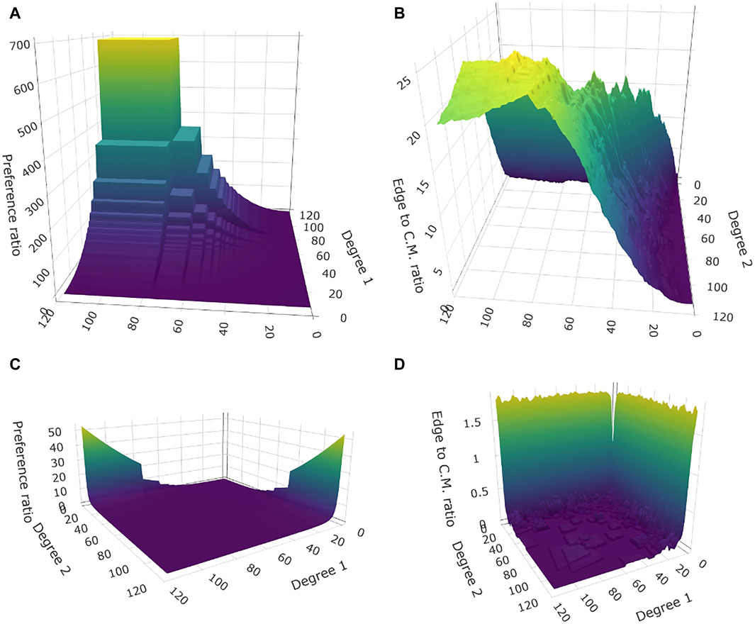
Figure 1
www.frontiersin.org

Figure 1. Networks built according to a preference function. Assortative network with γm,γM=1,1: normalized ratio between preference function and CM edge density (A), normalized ratio between the empirical and CM edge densities (B). Disassortative network with γm,γM=3,3: normalized ratio between preference function and CM edge density (C), normalized ratio between the empirical and CM edge densities (D).
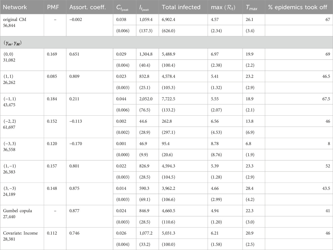
Table 1
www.frontiersin.org

Table 1. SIR epidemic summaries for each network type. Average values are based on 200 replicated epidemics, with standard deviation shown in brackets. Only epidemics that took off were included. tpeak refers to the time of maximum incidence, and Tmax is the maximum length of the epidemic. Size of the giant component is given below the network name.
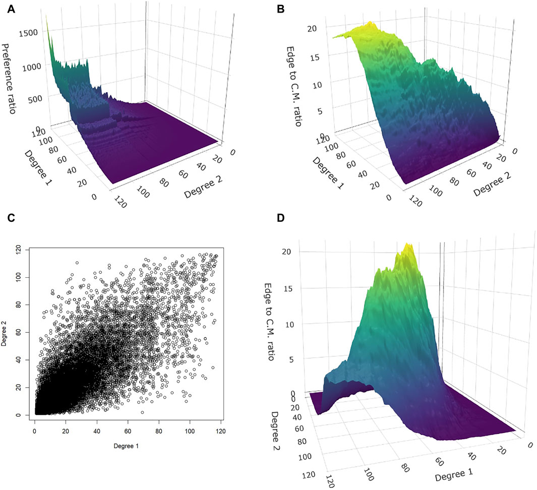
Figure 2
www.frontiersin.org

Figure 2. Covariate-induced network (income correlated with degree, ρ=0.6): normalized ratio between preference function and CM edge density (A), normalized ratio between the empirical and CM edge densities (B). Network built via Gumbel copula (θ=2): scatter plot of degrees (C), ratio between the empirical and CM edge densities (D).

3.2 SIR epidemic results

We run 200 epidemics on each of the generated networks, with transmissibility set at α=0.25, and visualize the resulting It and Rt by plotting against the cumulative fraction infected, Ct=1St. Supplementary Figure S2 illustrates that plotting It versus Ct leads to less variability in the process as opposed to plotting vs. time. This is because epidemics are driven by stochasticity in the beginning, i.e., whether they take off and when; however this all happens when Ct0, so it will not show in a plot against Ct. Showing Rt versus Ct can further reduce variability in the system since, at least in the CM network, It depends on It1 and Ct (via Rt), whereas Rt only depends on Ct. Notice from Supplementary Figure S2 that all Rt curves tend to be noisy at the beginning and end–due to small numbers of infected and hence the role of stochasticity –, but follow a fairly precise trajectory in the middle, where spread is deterministic.

Figure 3 shows two networks that exhibit qualitatively different epidemic curves. The network with a flat preference function, γm,γM=0,0 has the highest Rt values among all networks where epidemics take off (more on this below). This drives an explosive growth in infections at the beginning, after which Rt decays somewhat exponentially, compared to the CM where the decay in Rt looks linear. The network with γm,γM=3,3 is the network with the highest positive assortativity of all networks built via a preference function. What is interesting about the associated epidemics is both the shape of Rt (exponential, then linear), as well as how long the stochastic phase lasts: Rt does not become “deterministic” until about halfway through the epidemic.
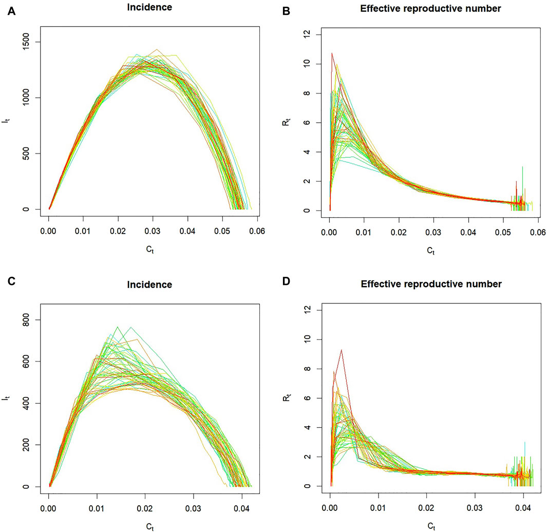
Figure 3
www.frontiersin.org

Figure 3. Examples of epidemics over two networks, one having γm,γM=0,0 (A,B), and another γm,γM=3,3 (C,D). Transmissibility is α=0.25; showing 100 realizations.

We record summary statistics from all epidemic experiments in Table 1. In particular, we are interested in the total number of infections, and in the epidemic curve profile, i.e., how long does the epidemic last, the size of the peak, and rate of growth at the beginning (typically indicated by maxRt, as the effective reproductive number tends to be highest at the beginning of the epidemic). These statistics exclude epidemics that die out in the initial stages. From these summaries we observe that the CM network is fairly good at spreading epidemics; most of the other networks result in smaller epidemics, and only two sustain a higher number of infections (by about 10%). The CM network also maintains an epidemic active for the longest time, except for the 3,3 network. The performance of the latter is surprising, given that it has one of the smallest epidemic sizes, as well as the smallest giant component.

We also investigate how the total size of an epidemic is affected by changes in transmissibility α. Figure 4 shows this monotonic relationship for three networks: the CM network, one assortative, and one disassortative. The curve for the disassortative network displays a kink around α=0.3. Below this value epidemics are limited in size, but above it, the linear trend takes over until the entire giant component is infected at α=1.
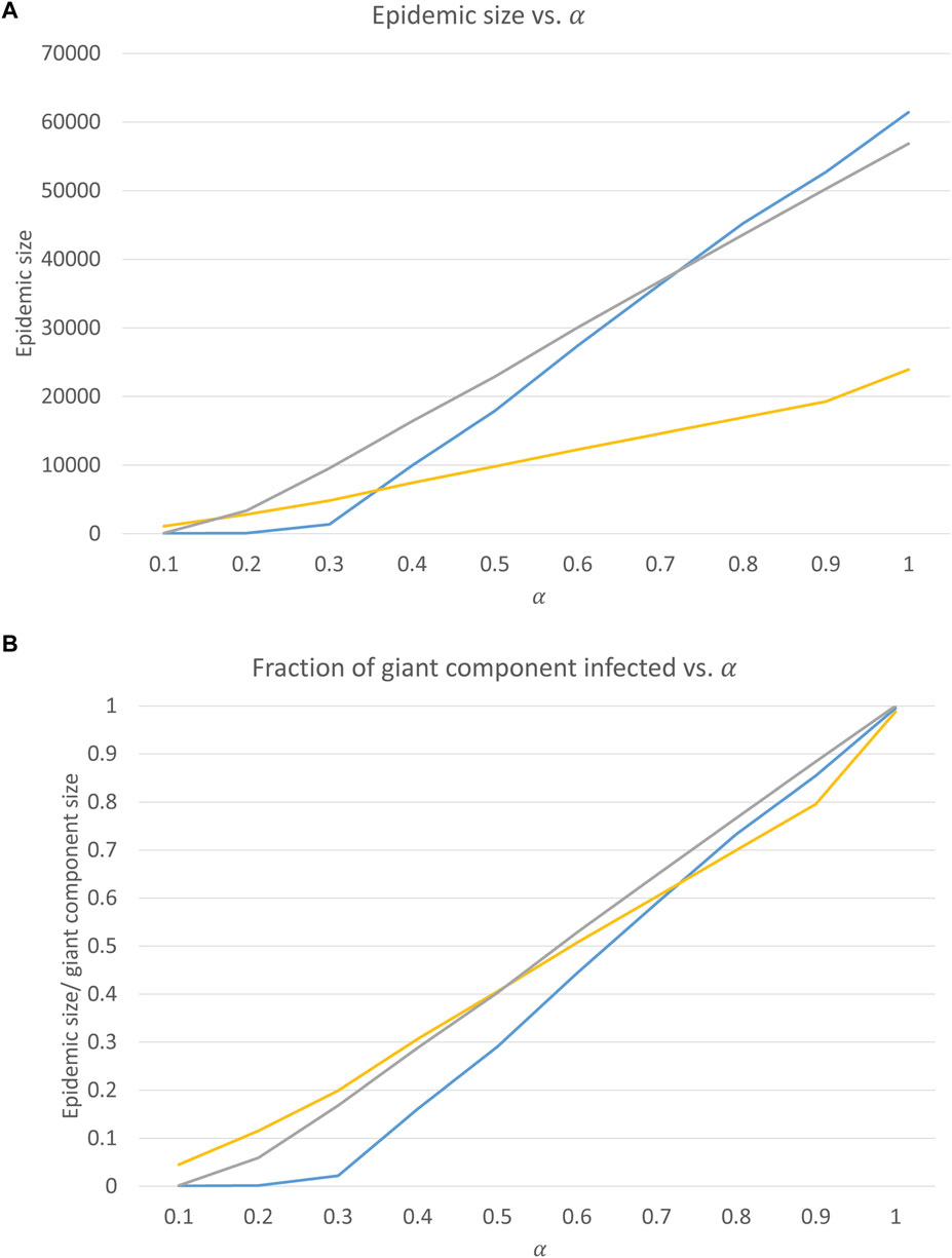
Figure 4
www.frontiersin.org

Figure 4. Epidemic sizes as a function of α for three networks: assortative (γm,γM=3,3, yellow), disassortative (γm,γM=2,2, blue), and neutral (CM network, grey). Sizes are given as counts of total infections (A), and as fractions of the giant components of the respective graphs (B).

4 Discussion

In this paper we introduced an algorithm to construct a network, based on the idea of preference to form an edge, given as a parametric function. The main advantage of preference functions is that they allow for a basic underlying mechanism for how the network is built, without being overly subject-specific, such as game-theoretic or ecological networks. This allows for some claim of plausibility or realism when building a network. This algorithm does not intend to replace existing rewiring algorithms, which are efficient when a matrix e is available, but rather it intends to offer a mechanistic explanation for the genesis of networks, when e is not known a priori. More generally, we have shown how a preference for degree can be extracted from a multivariate distribution of features which includes degree, and a general preference function (which may or may not depend on degree). By contrast, copulas are convenient and tractable models of joint dependence, but do not explain how a dependence structure emerges.

We have also investigated the spread of SIR epidemics on these networks, in an attempt to generate hypotheses for future work. The following conclusions and questions emerged:

• The second order structure of the graph (given in matrix e) has profound implications for the spread of disease. It can either help to prevent spread, to the point of effectively stopping an epidemic from reaching any meaningful size, on the lower range of α values.

• The effective reproductive number Rt seems to be predictable as a function of St in most cases, leading to the hypothesis that St provides a good description of the current state of the epidemic in time. In other words, knowing St and the average functional dependence of Rt on St enables prediction of the future epidemic trajectory without knowing the exact structure of the graph, or the past infection history (which vertices were infected and when).

• While the assortativity coefficient is meaningfully related to diffusion spread, it does not correlate with size of epidemics in a monotonic fashion. The question emerges of whether there is another graph summary that is more directly related to epidemic spread.

Data availability statement

The raw data supporting the conclusions of this article will be made available by the authors, without undue reservation.

Author contributions

RR: Conceptualization, Formal Analysis, Investigation, Methodology, Software, Visualization, Writing–original draft, Writing–review and editing.

Funding

The author(s) declare that financial support was received for the research, authorship, and/or publication of this article. This research received financial support from Research Manitoba, as part of its COVID-19 Research Fund. RR is based at the George and Fay Yee Centre for Healthcare Innovation. Support for CHI is provided by University of Manitoba, Canadian Institutes for Health Research, Province of Manitoba, and Shared Health Manitoba.

Conflict of interest

The author declares that the research was conducted in the absence of any commercial or financial relationships that could be construed as a potential conflict of interest.

Publisher’s note

All claims expressed in this article are solely those of the authors and do not necessarily represent those of their affiliated organizations, or those of the publisher, the editors and the reviewers. Any product that may be evaluated in this article, or claim that may be made by its manufacturer, is not guaranteed or endorsed by the publisher.

Supplementary material

The Supplementary Material for this article can be found online at: https://www.frontiersin.org/articles/10.3389/fphy.2024.1435767/full#supplementary-material

Footnotes

1In Newman’s original definition, eij is the fraction of edges connecting one vertex of type i to another of type j. On directed graphs, edges counted in eij are different from those counted in eji, and the condition i,jeij=1 is clearly satisfied. However, in undirected graphs eij=eji, and edges linking i to j vertices are counted twice in the sum i,j=1..Meij. So this literal interpretation of eij is problematic. The way Newman seems to think about this is to replace each edge in an undirected network by two directed edges going in opposite directions. In that case we end up with twice the number of edges, and the network consistency relationships in [14], i,jeij=1 checks out. Our adjustment to e makes double counting explicit, so there is no inconsistency.

2This corresponds to the 80–20 rule [27].

References

1. Callaway DS, Newman MEJ, Strogatz SH, Watts DJ. Network robustness and fragility: percolation on random graphs. Phys Rev Lett (2000) 85(25):5468–5471. doi:10.1103/PhysRevLett.85.5468

PubMed Abstract | CrossRef Full Text | Google Scholar

2. Newman MEJ. The structure and function of complex networks. SIAM Rev (2003) 45(2):167–256. doi:10.1137/S003614450342480

CrossRef Full Text | Google Scholar

3. Romanescu RG, Deardon R. Fast inference for network models of infectious disease spread. Scand J Stat (2017) 44(3):666–83. doi:10.1111/sjos.12270

CrossRef Full Text | Google Scholar

4. Miller JC, Slim AC, Volz EM. Edge-based compartmental modelling for infectious disease spread. J R Soc Interf (2012) 9(70):890–906. doi:10.1098/rsif.2011.0403

CrossRef Full Text | Google Scholar

5. Volz E. SIR dynamics in random networks with heterogeneous connectivity. J Math Biol (2008) 56(3):293–310. doi:10.1007/s00285-007-0116-4

PubMed Abstract | CrossRef Full Text | Google Scholar

6. Moreno Y, Vazquez A. Disease spreading in structured scale-free networks. EPJ B (2002) 31(2):265–271. doi:10.1140/epjb/e2003-00031-9

CrossRef Full Text | Google Scholar

7. Newman MEJ. Assortative mixing in networks. Phys Rev Lett (2002) 89(20):208701. doi:10.1103/PhysRevLett.89.208701

PubMed Abstract | CrossRef Full Text | Google Scholar

8. Kiss IZ, Green DM, Kao RR. The effect of network mixing patterns on epidemic dynamics and the efficacy of disease contact tracing. J R Soc Interf (2008) 5(24):791–9. doi:10.1098/rsif.2007.1272

CrossRef Full Text | Google Scholar

9. Wang Y, Chakrabarti D, Wang C, Faloutsos C. Epidemic spreading in real networks: an eigenvalue viewpoint. In: Proceedings of the IEEE Symposium on Reliable Distributed Systems (2003). p. 25–34. doi:10.1109/RELDIS.2003.1238052

CrossRef Full Text | Google Scholar

10. Kermack WO, McKendrick AG. A contribution to the mathematical theory of epidemics. In: Proceedings of the Royal Society of London. Series A, Containing Papers of a Mathematical and Physical Character, 115 (1927). p. 700–721. doi:10.1098/rspa.1927.0118

CrossRef Full Text | Google Scholar

11. Molloy M, Reed B. A critical point for random graphs with a given degree sequence. Random Struct Algorithms (1995) 6(2–3):161–80. doi:10.1002/rsa.3240060204

CrossRef Full Text | Google Scholar

12. Anderson I. B. Bollobás, random graphs (London mathematical society monographs, academic press, London, 1985), 447 pp., £52 cloth, £27 paper. In: Proceedings of the Edinburgh Mathematical Society, 30 (1987). p. 329. doi:10.1017/s0013091500028443

CrossRef Full Text | Google Scholar

13. Barabási AL, Albert R. Emergence of scaling in random networks. Science (1979) (1999) 286(5439):509–12. doi:10.1126/science.286.5439.509

CrossRef Full Text | Google Scholar

14. Newman MEJ. Mixing patterns in networks. Phys Rev E (2003) 67(2):026126. doi:10.1103/PhysRevE.67.0261269

CrossRef Full Text | Google Scholar

15. Xulvi-Brunet R, Sokolov IM. Construction and properties of assortative random networks. Phys Rev E (2004) 70(6):066102. doi:10.1103/PhysRevE.70.066102

CrossRef Full Text | Google Scholar

16. Chang SL, Piraveenan M, Prokopenko M. Impact of network assortativity on epidemic and vaccination behaviour. Chaos Solitons Fractals (2020) 140:110143. doi:10.1016/j.chaos.2020.110143

CrossRef Full Text | Google Scholar

17. Dipple S, Jia T, Caraco T, Korniss G, Szymanski BK. Assortative mating: encounter-network topology and the evolution of attractiveness. Sci Rep (2017) 7:45107. doi:10.1038/srep45107

PubMed Abstract | CrossRef Full Text | Google Scholar

18. Avin C, Keller B, Lotker Z, Mathieu C, Peleg D, Pignolet YA. Homophily and the glass ceiling effect in social networks. In: ITCS 2015 - Proceedings of the 6th Innovations in Theoretical Computer Science. Association for Computing Machinery, Inc (2015). p. 41–50. doi:10.1145/2688073.2688097

CrossRef Full Text | Google Scholar

19. Jiménez-Martínez A, Melguizo-López I. Making friends: the role of assortative interests and capacity constraints. J Econ Behav Organ (2022) 203:431–65. doi:10.1016/j.jebo.2022.09.016

CrossRef Full Text | Google Scholar

20. Murphy TJ, Swail H, Jain J, Anderson M, Awadalla P, Behl L, et al. The evolution of SARS-CoV-2 seroprevalence in Canada: a time-series study, 2020-2023. CMAJ Can Medical Assoc J (2023) 195(31):E1030–7. doi:10.1503/cmaj.230249

CrossRef Full Text | Google Scholar

21. Romanescu RG, Hu S, Nanton D, Torabi M, Tremblay-Savard O, Haque MA. The effective reproductive number: modeling and prediction with application to the multi-wave Covid-19 pandemic. Epidemics (2023) 44(Sep):100708. doi:10.1016/j.epidem.2023.100708

PubMed Abstract | CrossRef Full Text | Google Scholar

22. Wang C, Lizardo O, Hachen D, Strathman A, Toroczkai Z, Chawla NV. A dyadic reciprocity index for repeated interaction networks. Netw Sci (2013) 1(1):31–48. doi:10.1017/nws.2012.5

CrossRef Full Text | Google Scholar

23. Miller JW, Harrison MT. Exact sampling and counting for fixed-margin matrices. The Ann Stat (2013) 41(3). doi:10.1214/13-aos1131

CrossRef Full Text | Google Scholar

24. Sklar A. Fonctions de r{é}partition {à} {n} dimensions et leurs marges (Distribution functions of {n} dimensions and their marginals). Publications de l’Institut Statistique de l’Universit{é} de Paris (1959), vol. 8.

Google Scholar

25. Geenens G. Copula modeling for discrete random vectors. Dependence Model (2020) 8(1):417–40. doi:10.1515/demo-2020-0022

CrossRef Full Text | Google Scholar

26. Muñoz-Herrera M, Dijkstra J, Flache A, Wittek R. Collaborative production networks among unequal actors. Net Sci (2021) 9(1): 1–17. doi:10.1017/nws.2020.23

CrossRef Full Text | Google Scholar

27. Dunford R, Su Q, Tamang E, Wintour A. The Pareto principle. The Plymouth Student Scientist (2014) 7(2):140–148.

Google Scholar

28. Ruppert D. In Statistics and Data Analysis for Financial Engineering; Springer Texts in Statistics. New York, NY: Springer New York (2011). p. 175–200. doi:10.1007/978-1-4419-7787-8_8

CrossRef Full Text | Google Scholar

Keywords: graphs, degree distribution, edge matrix, assortative mixing, network construction, compartmental epidemic model

Citation: Romanescu RG (2024) Building a network with assortative mixing starting from preference functions, with application to the spread of epidemics. Front. Phys. 12:1435767. doi: 10.3389/fphy.2024.1435767

Received: 21 May 2024; Accepted: 15 July 2024;
Published: 05 August 2024.

Edited by:

Irina Severin, University POLITEHNICA of Bucharest, Romania

Reviewed by:

Konstantin Klemm, Spanish National Research Council (CSIC), Spain
Elena Corina Cipu, Politehnica University of Bucharest, Romania

Copyright © 2024 Romanescu. This is an open-access article distributed under the terms of the Creative Commons Attribution License (CC BY). The use, distribution or reproduction in other forums is permitted, provided the original author(s) and the copyright owner(s) are credited and that the original publication in this journal is cited, in accordance with accepted academic practice. No use, distribution or reproduction is permitted which does not comply with these terms.

*Correspondence: Razvan G. Romanescu, cmF6dmFuLnJvbWFuZXNjdUB1bWFuaXRvYmEuY2E=

Disclaimer: All claims expressed in this article are solely those of the authors and do not necessarily represent those of their affiliated organizations, or those of the publisher, the editors and the reviewers. Any product that may be evaluated in this article or claim that may be made by its manufacturer is not guaranteed or endorsed by the publisher.