 Anatol E. Wegner
- Center for Artificial Intelligence and Data Science, Julius Maximilian University of Würzburg, Würzburg, Germany
The prevalent approach to motif analysis seeks to describe the local connectivity structure of networks by identifying subgraph patterns that appear significantly more often in a network then expected under a null model that conserves certain features of the original network. In this article we advocate for an alternative approach based on statistical inference of generative models where nodes are connected not only by edges but also copies of higher order subgraphs. These models naturally lead to the consideration of latent states that correspond to decompositions of networks into higher order interactions in the form of subgraphs that can have the topology of any simply connected motif. Being based on principles of parsimony the method can infer concise sets of motifs from within thousands of candidates allowing for consistent detection of larger motifs. The inferential approach yields not only a set of statistically significant higher order motifs but also an explicit decomposition of the network into these motifs, which opens new possibilities for the systematic study of the topological and dynamical implications of higher order connectivity structures in networks. After briefly reviewing core concepts and methods, we provide example applications to empirical data sets and discuss how the inferential approach addresses current problems in motif analysis and explore how concepts and methods common to motif analysis translate to the inferential framework.
1 Introduction
The analysis of networks representing interactions and relations between sub-units has become one of the primary tools for analyzing complex systems. One of the main objectives in network analysis is to identify and characterize structural patterns in networks [1] and to relate these to the functional and dynamical features of the system. Over the years many widely observed features of complex networks such as heterogeneous degree distributions, degree correlations and community structure have been successfully incorporated into methods and models of complex networks.
The identification of basic building blocks in the form recurring microscopic patterns is crucial in the formulation of accurate models and descriptions of complex systems. Although the presence of repeated microscopic patterns, aka network motifs, is widely recognized to be a characteristic of many complex networks with important functional and dynamic implications, methods for characterizing and modelling local connectivity structures remain under developed when compared to other network features such as communities.
1.1 Quantifying local network structure
Many empirical networks contain certain small connectivity patterns also known as network motifs [2] in much higher numbers than one would expect on the basis of random graph models that assume (conditional) independence of edges. One prominent example is the prevalence of triangles in social networks that reflects the fact that an individual’s friends have an increased likelihood to be friends themselves [3]. Network motifs are also extensively studied in systems biology where they are believed to contribute to the function of networked systems by performing modular tasks [4]. The fact that biological networks of quite different species seem to contain the same and/or similar motifs has motivated the idea that network motifs are indicative of common network design principles in biological circuits to which these networks have converged to through the evolutionary process [5, 6]. While small scale network features are widely believed to play an important role in the structural and functional organization of networks, current methods for quantifying small scale network structures rely on hypothesis testing based on exhaustive enumeration of subgraphs which leads to complications when detecting larger motifs.
The quantification of local network structures poses particular challenges, not the least due to the large number of potential subgraphs that can be formed on even relatively small neighbourhoods. For instance, there are 11,117 non-isomorphic connected motifs on 8 vertices in the undirected case. The number of motifs grows even faster for directed graphs resulting in 9,364 connected motifs on just 5 vertices. As a result counting subgraphs quickly becomes an ineffective way of capturing local network features as the size of the subgraphs under consideration is increased. Moreover, subgraphs are coupled through a complex web of dependencies which further complicates the problem of providing a concise yet informative description of the local structure of networks. Furthermore, finding larger motifs in even moderately sized networks poses computational challenges due to the complexity of subgraph enumeration [7].
1.2 Current approaches to network motifs
The prevalent approach in motif analysis introduced by Milo et al. [2] relies on comparing induced subgraph counts in the original network to counts expected under a null model in the form of a graph ensemble that conserves some salient features of the original network. Usually, the feature to be conserved is picked to be the degree distribution resulting in configuration model type null models. The statistical significance of individual motifs is then determined by comparing the subgraph counts in the original network to the distribution of counts in a sample of the null model. Although the approach of Milo et al. has lead to significant insights into structure and function of complex networks is has some intrinsic limitations especially when considering larger motifs.
A major difficulty in motif analysis is that subgraph counts in networks are correlated in various ways [8–10]. One of the primary sources of correlations between subgraph counts are shared substructures. For instance, as already noted by Milo et al. [2], the presence of a large number of triangles in a network implies the presence of many 4-node subgraphs that contain triangles. In order to counter such effects Milo et al. proposed to conserve the counts of subgraphs of size
The interdependence of subgraph counts also leads to issues in the formulation and selection of null models that preserve certain features of the network since many widely used network measures, such as clustering, assortativity and degree distributions can be expressed in in terms of subgraph counts [12]. Consequently, expectation values of subgraph counts can vary significantly depending on the set of features that is selected as the basis of the null model.
Putting the problems of choosing an appropriate null model and the interdependence of subgraph counts aside, calculating the statistical significance of larger motifs is also computationally challenging because of the increased complexity that comes with enumerating larger subgraphs and the need to consider larger samples, due to the larger number of hypotheses being tested simultaneously, to achieve a certain level of statistical significance. In practice these compounding effects, limit the size of motifs that can be reliably detected via subgraph count based hypothesis testing [13–15] in even moderately sized networks.
In the light of these computational difficulties several alternative approaches for calculating the statistical significance of motifs have been explored in the literature which fall into two main categories: sampling methods and analytical approaches. While sampling methods can reduce the cost of subgraph enumeration by several orders of magnitude [16, 17] this inevitably comes at a cost of reduced accuracy. On the other hand analytical approaches [17–19] seek to obtain analytical approximations of the subgraph distributions under the null model with the aim of dispensing of the need to enumerate subgraphs in samples of the null model. However, analytical expressions for subgraph distributions are notoriously difficult to calculate for even the simplest of null models, such as the Erdös Rényi model. Consequently, analytical approaches rely on estimates of lower order moments of subgraph distributions which in turn require additional assumptions on the functional form of subgraph distributions in order to compute the statistical significance of motifs. One such example is the widely used the z-score [6] which implicitly assumes subgraph distributions to be Gaussian. However, subgraph distributions in random graphs are often far from being Gaussian making p-values derived from z-scores difficult to interpret [10, 18]. Although alternative distributions have been explored in the literature [18], in general subgraph distributions can vary significantly depending on the characteristics of the original network, the null model and the motif under consideration [10] which makes obtaining reliable p-values from lower order moments of subgraph distributions challenging.
1.3 Motifs and random graph models
The prevalence of network motifs in real world networks has also proven to be challenging for random graph models as most widely used random graph models assume that edges are conditionally independent, which for sparse models results in networks that are locally tree like. The lack of analytically solvable models that replicate local connectivity structures observed in empirical networks has also been an obstacle in the development of quantitative approaches for analysing local structures in networks and their topological and dynamical implications.
Classically, efforts for constructing models with nontrivial subgraph structures have focused on exponential random graph models (ERGM) which are maximum entropy models that result from constraining expected subgraph counts to their observed values. However, the inclusion of higher order subgraphs in ERGMs results in models with nonlinear interactions that are notoriously difficult to threat analytically and hence do not lend themselves easily to calculations and inference [20]. As a result, in practice one has to rely to Monte Carlo methods which themselves suffer from issues of inconsistency and degeneracy [21, 22] and finite sample effects [23]. Although there exist alternative formulations that seek to address some of these problems [20] in general ERGMs have mostly studied in cases where only a handful of pre-determined motifs, swuch as triangles, are included in the model. However, for ERGMs to be used as generative models in motif analysis one would need to consider ERGMs based on subgraph counts of arbitrary sets of motifs which at present seems unpractical.
Consequently, generative models that aim to replicate the prevalence of network motifs by connecting vertices not only by edges abut also copies of higher order subgraphs have emerged as an analytically tractable alternative to ERGMs [24–28]. These generative models share similarities with so called bipartite models for networks with group interactions such as collaboration networks [29] where one first generates a set of higher order interactions which are then projected onto edges to obtain a graph. Formulating models in terms of higher order subgraphs used to construct the network further enables the formulation of degree corrected models where not only the counts and types of atomic substructures but also the number of subgraphs attached to each vertex can be controlled. Such models in general more accurately reflect the structure of real world networks which often have highly heterogeneous degree distributions.
In the formulation of our method we rely on maximum entropy formulations of such models [28] that result from constraining the counts and distributions of higher order subgraphs used in the construction of the network. Assuming generative models of this type, one is naturally faced with the problem of determining the types of subgraphs and their distributions that are mostly likely to have resulted in the observed network, which is one of the main problems that the inferential approach addresses.
1.4 Higher order networks
Higher order networks are motivated by the observation that many systems can not faithfully represented by pairwise interactions only. Indeed, many complex systems include so called higher order interactions that involve more than two actors. For instance, proteins combine to form larger complexes, scientists collaborate in groups, groups of genes coordinate into modules to perform specific cellular functions, and economic and social agents can form complex coordinated groups with nontrivial internal structures with wide ranging structural and dynamical consequences [30–32].
Although many real networks are given as pairwise interactions in principle such networks should still reflect the presence of higher order interactions and hence it should be possible to extract information on higher order interactions present in the system from pairwise interaction data. Consequently, the inference of higher order representations from dyadic interactions is an active field of research [33, 34]. Most higher order network research focuses of higher order networks in the form of simplicial complexes or hypergraphs, where group interactions are modelled using cliques resulting in models where nodes participating in a higher order interaction interact with each other uniformly. Although focusing on cliques has the advantage of simplicity, we shall consider more general higher order networks where higher order interactions can take the form of arbitrary simply connected subgraphs which will allow us analyse directed networks as well as networks that do not contain large numbers of cliques.
1.5 Overview of the inference based approach
The inferential approach differs from the approach of Milo et al. in two key aspects. First, it is based on modelling motifs as explicit higher order interactions that occur in an optimal decomposition of the network into recurring subgraphs rather than counting subgraphs. Second, it is based on statistical inference of generative models rather than hypothesis testing with respect to a null model. For a discussion of inferential and null model based approaches in the context of community detection see [35].
The assumption that networks are made of recurring atomic subgraphs naturally leads us to consider objects that correspond to decompositions of networks into smaller subgraphs which we call subgraph configurations. In the context of the generative models we consider, subgraph configurations correspond to the latent states that describe the higher order subgraphs that were added to the graph during the generating process. In order to infer an optimal subgraph configuration for a given network we follow a Bayesian methodology based on a nonparametric prior for models parameters. This nonparametric prior allows us to infer decompositions of network into atomic building blocks without requiring any prior assumption on the types, frequencies or distributions of atomic subgraphs. As a result the method not only produces a set of statistically significant atomic subgraphs but also an explicit decomposition of the network into such basic building blocks.
Methodologically our method is related to inference based methods for community detection that use Stochastic Block Models (SBMs) as generative models. The use of the SBM [3] and its degree corrected variant [36] in conjunction with statistical inference techniques have resulted in principled methods for community detection [36–39] and have also been successfully applied to time dependent networks [40], generalized communities [39] and, multilayer networks [40].
In SBM based community detection the vertices of the graph are assumed to be partitioned into
The rest of the paper is structured as follows in Section 2 we briefly review the core concepts and ideas underlying the inferential approach [41] and discuss how concepts commonly used in motif analysis trasnlate to the inferential approach. Then in Section 3 we discuss empirical results for several real world networks and also analyse larger collections of similar networks. We conclude in Section 4 with a discussion of open problems and potential topics for future research.
2 Network motifs and subgraph decompositions
Following the original premise of Milo et al. of identifying basic building blocks of networks we seek identify such building blocks on the basis of how well a given network can be decomposed into them. Formalizing such an approach first requires a definition of what is meant by a decomposition into subgraphs and then the formulation of an objective function that can be used to discriminate between alternative decompositions of the same network.
In the following we briefly overview the inference based approach presented in [41] and then proceed to discuss how this approach addresses some of the problems in motif analysis. We also discuss how commonly used concepts in motif analysis translate to the inference based approach. We start with a high level overview of core concepts required to formulate the method and refer the reader to the respective references for further technical details.
2.1 Motifs, automorphisms and orbits
We start with a brief overview of basic graph theoretical concepts. Throughout this paper we use standard graph theoretic notation. For example, for a graph
The above definitions can be generalized to directed graphs in a straightforward manner, the only modification needed being that for directed graphs isomorphisms are also required to preserve edge directions. With this additional condition all definitions and expressions are valid both for directed and undirected networks.
2.2 Subgraph configurations
Definition 2.1:. (Subgraph configuration) Let
Given a subgraph configuration
Any subgraph configuration
Indeed many widely used graph representations are special cases of subgraph configurations. A trivial example is the edge list which is equivalent to the configuration that consists of all single edge subgraphs of
Figure 1. A subgraph configuration consisting of three edges, a triangle, a 4-cyles and two 4-diamonds.
2.3 Generative models
The formulation of our method is based on microcanonical ensembles which given a set of constraints on the types, counts and distributions of the subgraphs in a configuration assign all configurations that satisfy these constrains equal probability [28]. These models are closely related to other random graph models [24, 25, 27, 43] that rely on adding explicit copies of triangles and other higher order subgraphs to the graph during the generation process. One advantage of using microcanonical ensembles as generative models is that the parameters of the model are discrete and correspond to mutually exclusive constraints which when combined with discrete priors allow marginal probabilities to be calculated efficiently without requiring the computation of costly integrals.
Although the models we consider are similar to exponential random graphs in that they are maximum entropy ensembles the crucial difference is that subgraph configuration models constrain the subgraphs (i.e., building blocks) used to construct the network rather than subgraph counts in the network. This results in analytically tractable models that are generalizations of the Erdös-Rényi (ER) [44] and configuration models to higher order interactions. Though these models can be solved analytically for many of their properties in the context statistical inference we shall focus on the log-likelihood or entropy which can be calculated in closed form [28].
2.3.1 Homogeneous models
The simplest generative model that can be formulated for subgraph configurations on a set of vertices
where
where
The distribution over subgraph configurations given by homogeneous models can be transformed into a distribution over graphs by considering the distribution that arises from projecting subgraph configurations onto graphs by taking the union over all the edges contained in the subgraphs in
where
2.3.2 Degree corrected models
Homogeneous subgraph configuration models result in graphs with narrow– Poisson type degree distributions [25] in contrast to the heavy tailed degree distributions observed for many real world networks. Hence, we consider degree-corrected subgraph configuration models (DC-SGCM) which constrain not only the counts of atoms but also their distributions over vertices which can be done by specifying the number of atomic subgraphs attached to each vertex. Degree-corrected models are in general a better fit for most real world networks and therefore also improve the quality of the inferred configurations, similar to the effects observed in community detection based on the degree corrected SBM [36, 38].
Definition 2.2:. (Orbit degree) Given a subgraph configuration
In other words
As in the case of homogeneous models the microcanonical ensemble of subgraph configurations for a given orbit degree sequence
Specifying the degree distribution at the level of orbits can result in high dimensional degree distributions resulting in models with high parametric complexity. In order to reduce the number of parameters, the atomic degree distribution can be coarse grained at various level. One way of relaxing the DC-SGCM is to only specify the number of different atoms attached to each vertex without specifying their orbits i.e.,
Although the coarse grained versions of the DC-SGCM capture the propensity of vertices to attract subgraphs, it should be noted that the coarse grained versions do not conserve the edge degree distribution exactly since orbits in general have different degrees. At this stage one might wonder if it is possible to consider a subgraph configuration models where one conserves the degree sequence of the resulting graph instead of atomic degree sequence. Although in theory it is straightforward to formulate such models in terms of uniform ensembles of configurations of which have a given projected degree sequence, calculations of the likelihood of such models depends on non-negative solutions of systems of linear Diophantine equations for which no general solution is known.
Degree corrected subgraph configuration models can be sampled using a generalization of the well known half-edge matching algorithm for generating graphs with a prescribed degree sequence [24]. The only difference being that in the case of higher order subgraphs, in addition to half edges one needs to consider partial subgraphs or corners that need to be matched in appropriate combinations. Similarly, given a subgraph configuration with a certain atomic degree sequence it is possible to randomize/shuffle the configuration while preserving the degree sequence following a generalization of the edge swapping algorithm. Again, here the main difference is that the algorithm involves swapping pairs of corners corresponding to compatible orbits instead of only the endpoints of edges. Functions for generating and randomizing subgraph configurations provided as are part of our implementation of the method.
Being a generalization of the edge only configuration models, many techniques such as generating functions generalize to the higher order configuration models in a straightforward manner [24], allowing degree corrected models to be solved analytically for many of their properties ranging from spectral properties to percolation and component sizes [24, 25, 27, 46–48]. Despite having many desirable properties the use of such higher order configuration models has been constrained by the lack of techniques for fitting networks to these types of models which requires the determination of an appropriate set of higher order subgraphs
2.4 Statistical inference
Upon first inspection, it may not be immediately apparent whether a particular network can be decomposed into recurring subgraphs and, if such representations can be found how one can discriminate between them. In this section we provide a brief overview of how these questions can be addressed from the perspective of Bayesian inference. The Bayesian formulation can also be shown to be equivalent to the Minimum Description Length (MDL) approach and hence is equivalent to finding a subgraph configuration that represents the network most parsimoniously, i.e., with the least number of bits.
2.4.1 Nonparametric Bayesian inference
From the Bayesian perspective our goal is to infer a subgraph configuration that is most likely given the network
where
To formulate our prior we first consider the case of degree-corrected subgraph configuration models. For a given atomic degree sequence
where
For the sake of brevity we omit the exact forms of the priors and refer the reader to Ref. [41] for closed form expressions.
Having formulated the prior our goal becomes to find a subgraph configuration that has Maximum Posterior Probability (MAP)
2.4.2 Description length and statistical significance
The Bayesian formulation outlined above is equivalent to the Minimum Description Length (MDL) approach. Although the equivalence of the two approaches holds more broadly, in our case the equivalence is more directly evident due to the discrete nature of the parameters and the fact that for microcanonical models each configuration is compatible with a unique set of parameters. The Description Length (DL) is given by:
where
The description length can also be used to asses the statistical significance of the inferred MAP-configuration by comparing its description length to the description length of the configuration that contains no higher order subgraphs i.e., the configuration that consists of all single edges which is corresponds to the edge only configuration model:
Note that the above expression is well defined as the configuration consisting of only single edges is included in the prior which also ensures that the edge only configuration is selected if the network does not contain any statistically significant higher order motifs.
2.4.3 Statistical significance of motifs
While the reduction in description length
where
Normalized significance profiles are especially useful when comparing larger collections of networks containing networks that differ from one another in terms of size and density, as for instance in Section 3.3.
2.4.4 Model selection
Having one general form for the prior that is applicable to all model variants also allows for consistent model selection within an unified framework. For instance, let
The posterior odds ratio can be used to discriminate between different variants of the degree corrected SGCMs as well homogeneous models [41], allowing us to select the optimal model and corresponding MAP-configuration for a given network.
2.5 Inference algorithm
Finding a MAP-configuration is a set covering problem [49] where the goal is to cover the set
where
The computational complexity of finding a MAP configuration is dominated by the step of finding a maximum set of edge-independent
The current implementation relies on the LAD algorithm [50] for subgraph isomorphism search but in principle is compatible with any subgraph isomorphism algorithm, including algorithms such as TurboISO [51] and DAF [52] which are known to scale better to larger graphs.
One advantage of the inference based approach is that inference algorithms can be tested on simulated data with a known underlying subgraph configuration. When tested on such data sets the algorithm is able to recover the underlying latent states to a high degree of accuracy [41].
3 Empirical results
In this section we provide examples of empirical results for two empirical networks a directed human connectome from [53] and a network of protein-protein interactions (PPI) in Drosophila melanogaster [54]. Due to computational constraints we limit the size of motifs to up to 8 nodes for undirected networks and up to 5 in the directed case. This corresponds to 9,578 potential motifs in the directed case and 12,112 in the undirected case. Despite the large number of potential motifs the method is able to infer concise sets of atoms for both of these networks. We then also analyse large sets of directed and undirected connectomes of the human brain and, protein interaction networks. Additional examples including neural networks, collaboration networks and metabolic networks can be found in [41].
3.1 Human connectome
The directed connectome of the human brain [53] we consider has 1,015 vertices and 3,787 edges and the MAP-configuration, inferred using the directed degree corrected SGCM, contains 22 non-trivial patterns which cover approximately 75% of all edges (see Figure 2). The MAP-configuration has a description length of 28,811 bits, a reduction of 1,927 bits over the edge only configuration model, from which means that the MAP-configuration is
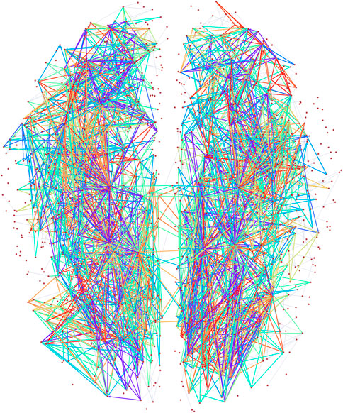
Figure 2. Visualization of the higher order subgraphs in the MAP configuration of the directed human connectome with edges coloured according the types of atoms. Node positions reflect physical locations of the brain regions in a 2D (horizontal) projection.
The MAP-configuration of the human connectome contains a large number of feed-forward loops (FFL) (Atom 1 in Table 1) and so called bi–fan motifs (Atoms 2 and 7 in Table 1) usually associated with neuronal networks [55]. We also find a large numbers of 4 and 5 node bi-parallel motifs (Atoms 3 and 6 in Table 1) where an input node is connected to an output node via indirect connections. In addition to these basic types we also recover more complex atoms that can be interpreted as various combinations of lower order atoms. Such larger arrangements of motifs have recently been analysed in [56] though our result show that in the human connectome lower order motifs in general combine in denser and more complex patterns than the pairwise combinations studied in [56] (Atoms 8–22 in Table 1). In addition we observe that all atoms contain at least one node with only incoming links and one node with only outgoing links which could interpreted as output and input nodes.
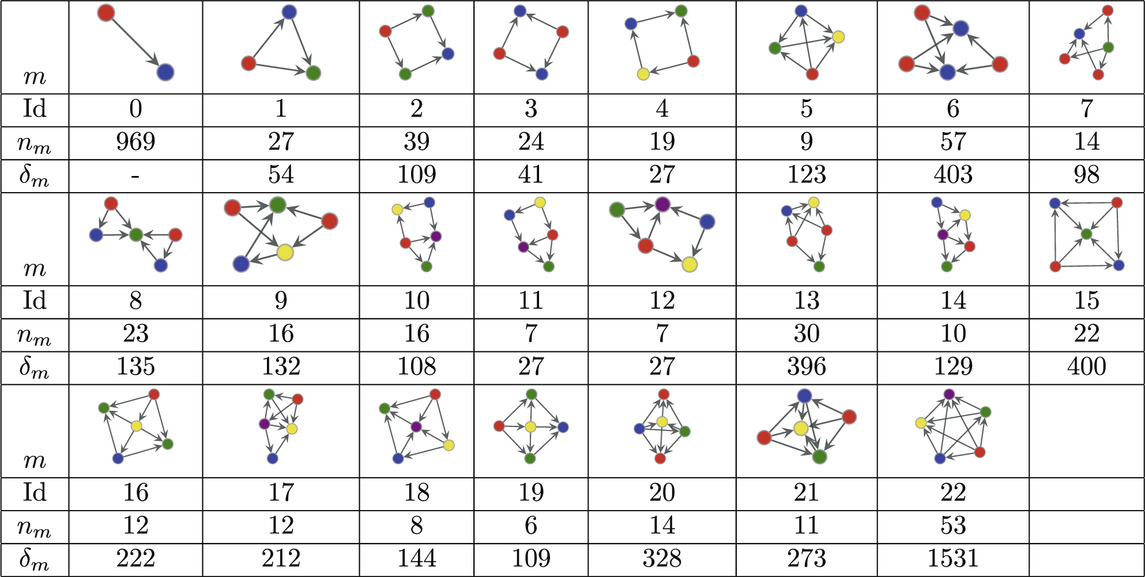
Table 1. Atoms found in the MAP configuration of the directed human connectome together with their respective counts
On the directed human connectome the greedy algorithms takes
In comparison, applying the approach of Milo et al. with a sample size of 1,000 and a threshold of 10 for the z-score to the same networks yields 114 motifs of size 5, 9 motifs of size 4 and 1 motif of size 3. Here, we opted for the use of the z-score, despite its known shortcomings, as a direct count based analysis would require enumerating subgraphs up to size 5 (
3.2 PPI network of Drosophila melanogaster
The PPI network of Drosophila melanogaster we consider has 2,939 vertices and 8,569 edges [54]. For this network the degree corrected model that constrains the total number of subgraphs attached to each vertex results in the shortest description length. The MAP-configuration of the network obtained from motifs up to size 8 contains 15 non-trivial patterns in addition to single edges which cover approximately 45% of all edges. A plot of the MAP-configuration is given in Figure 3. The MAP-configuration has a description length of 72,205 bits which corresponds to a reduction of 710 bits over the edge only configuration model. Hence, compared to the edge only configuration, the MAP-configuration is
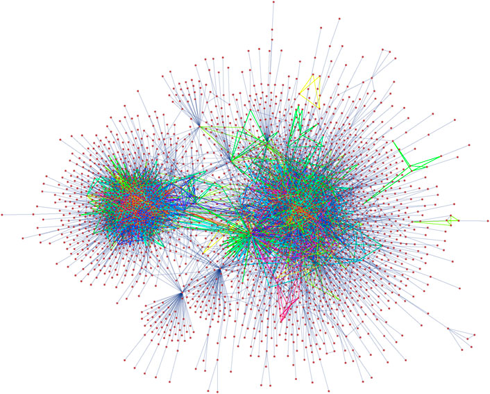
Figure 3. Visualization of the largest connected component of the PPI network of Drosophila melanogaster with edges coloured according to atomic subgraph type.
The MAP-configuration of the PPI network contains a large number bipartite cliques (Atoms 2, 4, 6, 9, and 12 in Table 2). These bipartite and multi-partite atoms (Atoms 5 and 15 in Table 2) can naturally be explained by the presence of shared interacting subdomains in proteins [57] that result in groups of proteins that interact with the same set of proteins but not among themselves. In addition we also recover cubic atoms (Atoms 7, 8, 10, 11, and 14 in Table 2) that are compatible with the formation of protein complexes in 3 dimensional space. In principle these results could be checked further by examining if the individual instances of these motifs in the MAP-configuration indeed coincide with known protein complexes or are results of shared subdomains. However, this requires expert domain knowledge and shall be explored in future research.
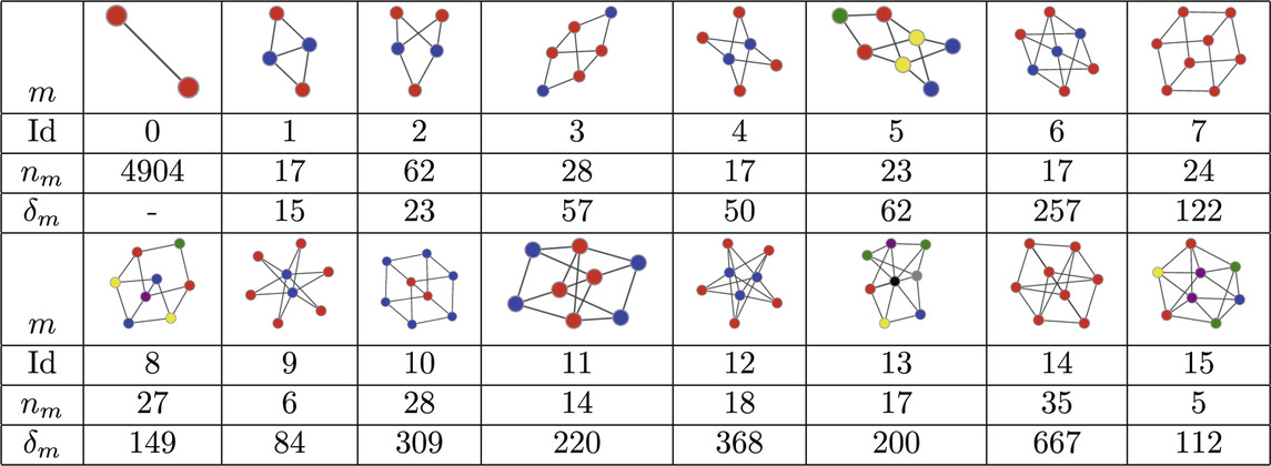
Table 2. Atoms found in the MAP-configuration of the PPI network of Drosophila melanogaster and their respective counts
For reference on the PPI network the greedy algorithms takes
Applying the method of Milo et al. with motifs of size 8 to this network is computationally not feasible hence we omit the comparison.
3.3 Network families
In this section we apply our method to large collections of networks representing similar systems namely directed and undirected connectomes of the human brain and, protein interaction networks. We compare the inferred MAP configurations obtained for the networks using normalized significance profiles introduced in Section 2.4.3. Our results show that the method produces consistent results across the networks in these datasets providing further support that the method is able to identify patterns that are characteristic to these networks. For, the directed networks we use the directed degree corrected SGCM and for the undirected networks we use the model variant that constrains the total number of subgraphs attached to each vertex, which are the model variants favoured by model selection on these datasets.
3.3.1 Directed human connectomes
The dataset of directed connectomes [53] consists of 423 networks corresponding to different experimental subjects. While all networks in this data set have 1,015 nodes corresponding to specific brain regions the number of edges ranges from 3,305 to 4,835. To compute the significance profiles we use the MAP configurations obtained using bi-connected motifs up to size 4 (138 potential motifs). The significance profiles for the directed human connectomes are given in Figure 4 and the corresponding atoms are given in Table 3. Despite variations in density of the networks we observe that the significance profiles of the 423 directed connectomes are in remarkable agreement the main difference being in the significance of atoms that correspond to pairwise combinations of FFLs (atoms 7, 8, and 10 in Table 3).
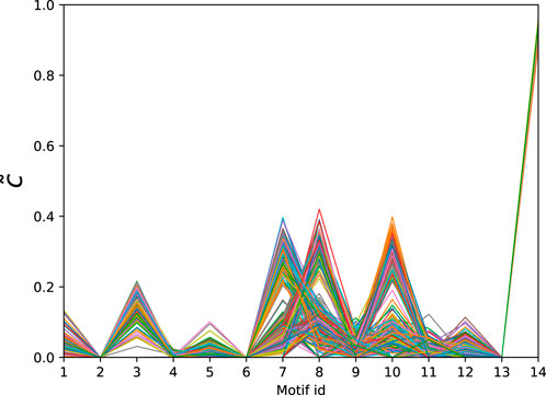
Figure 4. Normalised significance profiles of 423 directed human connectomes. The corresponding motifs can be found in Table 3.
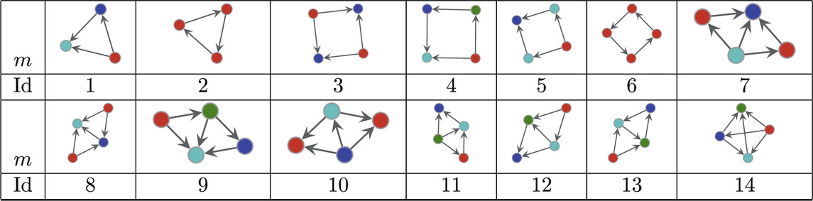
Table 3. Directed atoms found in the MAP-configurations of 423 directed human connectomes. The IDs correspond to the
3.3.2 Undirected human connectomes
Next we consider a collection of human connectomes from [58] containing 127 human connectomes with 445 nodes each and edge counts ranging from 3,527 to 5,722. In order to obtain the significance profiles we compute the MAP-configurations based on motifs up to size 5 (30 potential motifs). As in the directed case the normalised significance profiles (Figure 5) are remarkably similar across all networks with the main differences being in the significance of atoms 7, 8, and 9 (see Table 4).
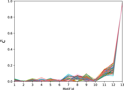
Figure 5. Normalised significance profiles of 127 undirected human connectomes. The corresponding motifs can be found in Table 4.
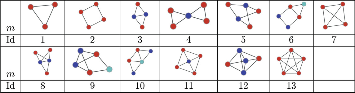
Table 4. Atoms found in the MAP-configurations of 127 undirected human connectomes- the IDs correspond to the
3.3.3 Protein-protein interaction networks
Finally, we consider a data set of PPI networks from [59] consisting of 335 networks corresponding to different species. The number of nodes ranges from 1,004 to 1,994 and the number of edges varies from 2,280 to 54,247. The normalised significance profiles of the MAP-configurations obtained with bi-connected motifs up top 5-nodes (15 potential motifs) are given in Figure 6. Again we find that the significance profiles are very similar with the exception of a few outliers that correspond to species that have only limited coverage.
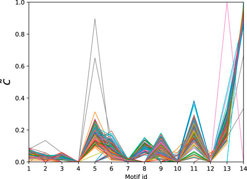
Figure 6. Normalised significance profiles of 335 PPI networks across diverse domains of the tree of life. The corresponding motifs are given in Table 5.
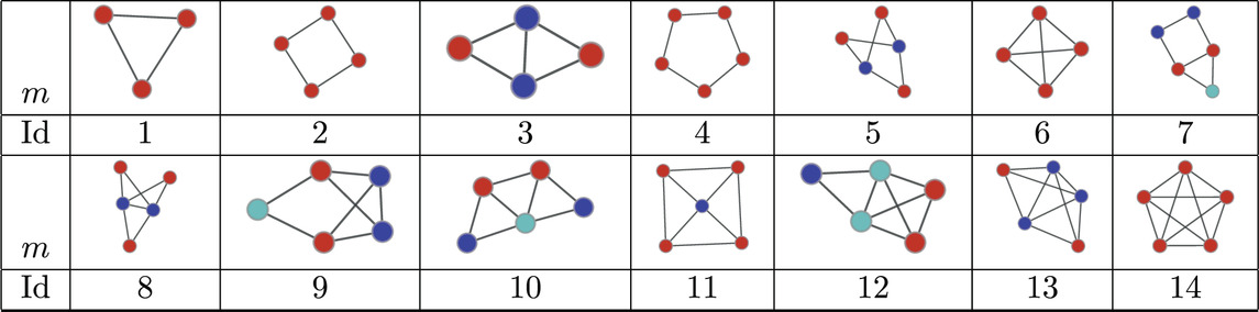
Table 5. Atoms found in the MAP-configurations of 335 PPI networks. The IDs correspond to the
4 Discussion
4.1 Summary
In this article, we presented an alternative perspective on network motifs, grounded in the modeling motifs through higher-order interactions and nonparametric inference techniques for obtaining an optimal set of higher order interactions. The inferential approach offers several advantages over traditional count-based methods. Firstly, our method produces an explicit decomposition of networks into higher-order building blocks. This not only offers an alternative interpretation of network motifs as fundamental building blocks of networks but also allows for the examination of individual motif instances within the context of the whole network. Additionally, these higher-order representations can be used to formulate dynamical models to study the dynamical implications of higher-order structures in real world networks [30] even if these networks are initially given in terms of pairwise interactions.
Moreover, from an algorithmic standpoint our approach does not require exhaustive subgraph enumeration and is trivially parallelizable enabling the detection of larger motifs while still producing concise and highly interpretable sets of motifs. Importantly, the method shows that many real-world networks can be represented more parsimoniously by including higher-order interactions into their representations, even if the data initially contains only pairwise interactions opening new avenues for the application of higher order network analysis methods to dyadic networks.
Being grounded in statistical inference, the method provides an effective approach for identifying larger motifs by considering all motifs simultaneously within a single generative model generative model, regardless of their size or other characteristics. The nonparametric Bayesian approach allows for the formulation of general and expressive priors and naturally safeguards against over-fitting producing interpretable and robust results. This allows the method to infer concise sets of motifs that have high statistical significance, even when the numbers of potential motifs is very large.
Finally, our method also provides a fit of the network to analytically tractable generative models that reflect the inferred higher-order structures. These models can be used to generate samples of networks that share the higher order organization of the original network and further allow distribution and prevalence of motifs in the model to be varied in a controlled manner. This opens new avenues for systematically studying the topological and dynamical implications of higher order structures in networks [30, 32], and could provide valuable insights into network behaviour.
In summary, our approach offers a powerful framework not only for detecting meaningful higher-order structures in networks but also for studying their topological and dynamical implications.
4.2 Open problems and future directions
Temporal and multilayer networks pose additional challenges in motif analysis as the number of potential motifs in temporal [60–62] and multilayer networks [63] increases even faster with size than in static/single layer networks. In the context of such networks inference based approaches similar to the one presented here could prove useful due to their inherent ability to effectively balance goodness of fit and model complexity. While the generalization of higher order interactions to multilayer networks can be achieved by simply considering multilayer patterns, the generalization to temporal networks is likely to require further developments that additionally take both the duration and temporal order of interactions into account.
Another problem when detecting motifs is that network structures at different scales influence each other in various ways. For instance, the presence of modular structures influences subgraph counts, similarly the presence of triangles and other motifs can interfere with community detection algorithms that rely on the assumption that networks are tree-like at the local level. Hence, more realistic generative models that combine structures at various scales could provide the basis for improved methods and could provide a more complete picture of network structures across various scales.
The current implementation of the method relies on a greedy heuristic for finding MAP-configurations. The greedy heuristic involves iterating over all motifs up to a certain size which is a limiting factor for the size of the motifs that can be considered in the analysis due to the explosion in the number of candidate motifs. For instance, there are
Data availability statement
Publicly available datasets were analyzed in this study. This data can be found here: https://github.com/AnatolWegner/HigherOrderMotifs, https://pitgroup.org/connectome/, https://networks.skewed.de/.
Ethics statement
Ethical approval was not required for the study involving humans in accordance with the local legislation and institutional requirements. Written informed consent to participate in this study was not required from the participants or the participants’ legal guardians/next of kin in accordance with the national legislation and the institutional requirements.
Author contributions
AW: Conceptualization, Data curation, Methodology, Software, Visualization, Writing–original draft, Writing–review and editing, Formal Analysis.
Funding
The author(s) declare that no financial support was received for the research, authorship, and/or publication of this article.
Conflict of interest
The authors declare that the research was conducted in the absence of any commercial or financial relationships that could be construed as a potential conflict of interest.
Publisher’s note
All claims expressed in this article are solely those of the authors and do not necessarily represent those of their affiliated organizations, or those of the publisher, the editors and the reviewers. Any product that may be evaluated in this article, or claim that may be made by its manufacturer, is not guaranteed or endorsed by the publisher.
References
1. Newman M, Barabási A-L, Watts DJ. The structure and dynamics of networks. Princeton, New Jersey: Princeton University Press (2006).
2. Milo R, Shen-Orr S, Itzkovitz S, Kashtan N, Chklovskii D, Alon U. Network motifs: simple building blocks of complex networks. Science (2002) 298(5594):824–7. doi:10.1126/science.298.5594.824
3. Wasserman S. Social network analysis: methods and applications. Cambridge: Cambridge University Press (1994).
4. Alon U. Biological networks: the tinkerer as an engineer. Science (2003) 301:1866–7. doi:10.1126/science.1089072
5. Alon U. Network motifs: theory and experimental approaches. Nat Rev Genet (2007) 8(6):450–61. doi:10.1038/nrg2102
6. Milo R, Itzkovitz S, Kashtan N, Levitt R, Shen-Orr S, Ayzenshtat I, et al. Superfamilies of evolved and designed networks. Science (2004) 303(5663):1538–42. doi:10.1126/science.1089167
7. Ribeiro P, Paredes P, Silva ME, Aparicio D, Silva F. A survey on subgraph counting: concepts, algorithms, and applications to network motifs and graphlets. ACM Comput Surv (Csur) (2021) 54(2):1–36. doi:10.1145/3433652
8. Itzkovitz S, Milo R, Kashtan N, Ziv G, Alon U. Subgraphs in random networks. Phys Rev E (2003) 68(2):026127. doi:10.1103/physreve.68.026127
9. Ginoza R, Mugler A. Network motifs come in sets: correlations in the randomization process. Phys Rev E (2010) 82(1):011921. doi:10.1103/physreve.82.011921
10. Fodor J, Brand M, Stones RJ, Buckle AM. Intrinsic limitations in mainstream methods of identifying network motifs in biology. BMC bioinformatics (2020) 21:165–11. doi:10.1186/s12859-020-3441-x
11. Fischer R, Leitão JC, Peixoto TP, Altmann EG. Sampling motif-constrained ensembles of networks. Phys Rev Lett (2015) 115:188701–10. doi:10.1103/physrevlett.115.188701
12. Olbrich E, Kahle T, Bertschinger N, Ay N, Jost J. Quantifying structure in networks. Eur Phys J B (2010) 77:239–47. doi:10.1140/epjb/e2010-00209-0
13. Grochow JA, Kellis M. Network motif discovery using subgraph enumeration and symmetry-breaking. In: Research in computational molecular biology, Heidelberg, Germany. Berlin, Germany: Springer (2007). 92–106.
14. Patra S, Mohapatra A. Review of tools and algorithms for network motif discovery in biological networks. IET Syst Biol (2020) 14(4):171–89. doi:10.1049/iet-syb.2020.0004
15. Masoudi-Nejad A, Schreiber F, Kashani ZRM. Building blocks of biological networks: a review on major network motif discovery algorithms. IET Syst Biol (2012) 6(5):164–74. doi:10.1049/iet-syb.2011.0011
16. Kashtan N, Itzkovitz S, Milo R, Alon U. Efficient sampling algorithm for estimating subgraph concentrations and detecting network motifs. Bioinformatics (2004) 20(11):1746–58. doi:10.1093/bioinformatics/bth163
17. Wernicke S. Efficient detection of network motifs. IEEE/ACM Trans Comput Biol Bioinformatics (2006) 3(4):347–59. doi:10.1109/tcbb.2006.51
18. Picard F, Daudin J-J, Koskas M, Schbath S, Robin S. Assessing the exceptionality of network motifs. J Comput Biol (2008) 15(1):1–20. doi:10.1089/cmb.2007.0137
19. Squartini T, Garlaschelli D. Analytical maximum-likelihood method to detect patterns in real networks. New J Phys (2011) 13(8):083001. doi:10.1088/1367-2630/13/8/083001
20. D Lusher, J Koskinen, and G Robins editors. Exponential random graph models for social networks. Cambridge: Cambridge University Press (2012).
21. Chatterjee S, Diaconis P. Estimating and understanding exponential random graph models. The Ann Stat (2013) 41(5):2428–61. doi:10.1214/13-aos1155
22. Shalizi CR, Rinaldo A. Consistency under sampling of exponential random graph models. Ann Stat (2013) 41(2):508–35. doi:10.1214/12-aos1044
23. Hunter DR, Goodreau SM, Handcock MS. Goodness of fit of social network models. J Am Stat Assoc (2008) 103:248–58. doi:10.1198/016214507000000446
24. Karrer B, Newman M. Random graphs containing arbitrary distributions of subgraphs. Phys Rev E (2010) 82(6):066118. doi:10.1103/physreve.82.066118
25. Bollobás B, Janson S, Riordan O. Sparse random graphs with clustering. Random Structures and Algorithms (2011) 38(3):269–323. doi:10.1002/rsa.20322
26. Newman M. Random graphs with clustering. Phys Rev Lett (2009) 103(5):058701. doi:10.1103/physrevlett.103.058701
27. Miller JC. Percolation and epidemics in random clustered networks. Phys Rev E (2009) 80(2):020901. doi:10.1103/physreve.80.020901
28. Wegner AE, Olhede S. Atomic subgraphs and the statistical mechanics of networks. Phys Rev E (2021) 103:042311–4. doi:10.1103/physreve.103.042311
29. Newman ME. The structure of scientific collaboration networks. Proc Natl Acad Sci (2001) 98(2):404–9. doi:10.1073/pnas.98.2.404
30. Battiston F, Cencetti G, Iacopini I, Latora V, Lucas M, Patania A, et al. Networks beyond pairwise interactions: structure and dynamics. Phys Rep (2020) 874:1–92. doi:10.1016/j.physrep.2020.05.004
31. Boccaletti S, De Lellis P, Del Genio C, Alfaro-Bittner K, Criado R, Jalan S, et al. The structure and dynamics of networks with higher order interactions. Phys Rep (2023) 1018:1–64. doi:10.1016/j.physrep.2023.04.002
32. Majhi S, Perc M, Ghosh D. Dynamics on higher-order networks: a review. J R Soc Interf (2022) 19(188):20220043. doi:10.1098/rsif.2022.0043
33. Lambiotte R, Rosvall M, Scholtes I. From networks to optimal higher-order models of complex systems. Nat Phys (2019) 15(4):313–20. doi:10.1038/s41567-019-0459-y
34. Young JG, Petri G, Peixoto TP. Hypergraph reconstruction from network data. Commun Phys (2021) 4(12):135. doi:10.1038/s42005-021-00637-w
35. Peixoto TP. Descriptive vs. inferential community detection in networks: pitfalls, myths and half-truths. Cambridge: Cambridge University Press (2023).
36. Karrer B, Newman MEJ. Stochastic blockmodels and community structure in networks. Phys Rev E (2011) 83(1):016107. doi:10.1103/physreve.83.016107
37. Peixoto TP. Nonparametric bayesian inference of the microcanonical stochastic block model. Phys Rev E (2017) 95(1):012317. doi:10.1103/physreve.95.012317
38. Peixoto TP. Parsimonious module inference in large networks. Phys Rev Lett (2013) 110(14):148701. doi:10.1103/physrevlett.110.148701
39. Newman M, Peixoto TP. Generalized communities in networks. Phys Rev Lett (2015) 115:088701–8. doi:10.1103/physrevlett.115.088701
40. Peixoto TP. Inferring the mesoscale structure of layered, edge-valued, and time-varying networks. Phys Rev E (2015) 92:042807. doi:10.1103/physreve.92.042807
41. Wegner AE, Olhede SC. Nonparametric inference of higher order interaction patterns in networks. Commun. Phys. (2024) 7:258. doi:10.1038/s42005-024-01736-0
42. Royer L, Reimann M, Andreopoulos B, Schroeder M. Unraveling protein networks with power graph analysis. PLoS Comput Biol (2008) 4(7):e1000108. doi:10.1371/journal.pcbi.1000108
43. Guillaume J-L, Latapy M. Bipartite structure of all complex networks. Inf Process Lett (2004) 90(5):215–21. doi:10.1016/j.ipl.2004.03.007
44. Erdös P, Rényi A. On the evolution of random graphs. Publ Math Inst Hungar Acad Sci (1960) 5:17–61.
45. Wegner AE. Subgraph covers: an information-theoretic approach to motif analysis in networks. Phys Rev X (2014) 4(4):041026. doi:10.1103/physrevx.4.041026
46. Newman M. Spectra of networks containing short loops. Phys Rev E (2019) 100(1):012314. doi:10.1103/physreve.100.012314
47. Cantwell GT, Newman MEJ. Message passing on networks with loops. Proc Natl Acad Sci USA (2019) 116:23398–403. doi:10.1073/pnas.1914893116
48. Keating LA, Gleeson JP, O’Sullivan DJ. A generating-function approach to modelling complex contagion on clustered networks with multi-type branching processes. J Complex Networks (2023) 11(6):cnad042. doi:10.1093/comnet/cnad042
49. Chvatal V. A greedy heuristic for the set-covering problem. Mathematics operations Res (1979) 4(3):233–5. doi:10.1287/moor.4.3.233
50. Solnon C. Alldifferent-based filtering for subgraph isomorphism. Artif Intelligence (2010) 174(12–13):850–64. doi:10.1016/j.artint.2010.05.002
51. Han W-S, Lee J, Lee J-H. Turboiso: towards ultrafast and robust subgraph isomorphism search in large graph databases. In: Proceedings of the 2013 ACM SIGMOD international conference on management of data; 2013 June 22–27; New York, NY (2013). 337–48.
52. Han M, Kim H, Gu G, Park K, Han W-S. Efficient subgraph matching: harmonizing dynamic programming, adaptive matching order, and failing set together. In: Proceedings of the 2019 international conference on management of data; 2019 June 30–July 5; Amsterdam, Netherlands (2019). 1429–46.
53. Kerepesi C, Szalkai B, Varga B, Grolmusz V. How to direct the edges of the connectomes: dynamics of the consensus connectomes and the development of the connections in the human brain. PLoS One (2016) 11(6):e0158680. doi:10.1371/journal.pone.0158680
54. Tang H-W, Spirohn K, Hu Y, Hao T, Kovács IA, Gao Y, et al. Next-generation large-scale binary protein interaction network for drosophila melanogaster. Nat Commun (2023) 14(1):2162–16. doi:10.1038/s41467-023-37876-0
55. Kashtan N, Itzkovitz S, Milo R, Alon U. Topological generalizations of network motifs. Phys Rev E (2004) 70(3):031909. doi:10.1103/physreve.70.031909
56. Adler M, Medzhitov R. Emergence of dynamic properties in network hypermotifs. Proc Natl Acad Sci (2022) 119(32):e2204967119. doi:10.1073/pnas.2204967119
57. Moon HS, Bhak J, Lee KH, Lee D. Architecture of basic building blocks in protein and domain structural interaction networks. Bioinformatics (2005) 21(8):1479–86. doi:10.1093/bioinformatics/bti240
58. Roncal WG, Koterba ZH, Mhembere D, Kleissas DM, Vogelstein JT, Burns R, et al. Migraine: mri graph reliability analysis and inference for connectomics. In: 2013 IEEE global conference on signal and information processing; 2013 Dec 03–05; Austin, TX. IEEE (2013). 313–6.
59. Zitnik M, Sosič R, Feldman MW, Leskovec J. Evolution of resilience in protein interactomes across the tree of life. Proc Natl Acad Sci (2019) 116(10):4426–33. doi:10.1073/pnas.1818013116
60. Kovanen L, Karsai M, Kaski K, Kertész J, Saramäki J. Temporal motifs in time-dependent networks. J Stat Mech Theor Exp (2011) 2011(11):P11005. doi:10.1088/1742-5468/2011/11/p11005
61. Paranjape A, Benson AR, Leskovec J. Motifs in temporal networks. In: Proceedings of the tenth ACM international conference on web search and data mining; 2017 Feb 6–10; Cambridge, United Kingdom (2017). 601–10.
62. Liu P, Guarrasi V, Sarıyüce AE. Temporal network motifs: models, limitations, evaluation. IEEE Trans Knowledge Data Eng (2021) 35(1):945–57. doi:10.48550/arXiv.2005.11817
Keywords: network motifs, higher order networks, statistical inference, random graph models, network analysis, network module division
Citation: Wegner AE (2024) Modelling network motifs as higher order interactions: a statistical inference based approach. Front. Phys. 12:1429731. doi: 10.3389/fphy.2024.1429731
Received: 08 May 2024; Accepted: 05 August 2024;
Published: 27 August 2024.
Edited by:
Petter Holme, Aalto University, FinlandReviewed by:
Alfredo Pulvirenti, University of Catania, ItalyYilun Shang, Northumbria University, United Kingdom
Copyright © 2024 Wegner. This is an open-access article distributed under the terms of the Creative Commons Attribution License (CC BY). The use, distribution or reproduction in other forums is permitted, provided the original author(s) and the copyright owner(s) are credited and that the original publication in this journal is cited, in accordance with accepted academic practice. No use, distribution or reproduction is permitted which does not comply with these terms.
*Correspondence: Anatol E. Wegner, YW5hdG9sLndlZ25lckB1bmktd3VlcnpidXJnLmRl