Sensitivity analysis of non-uniform rational B-splines–based finite element/boundary element coupling in structural-acoustic design

For the purpose of modeling the acoustic fluid-structure interaction using direct differentiation method and conducting a structural-acoustic sensitivity analysis, a coupling approach based on the finite element method and the fast multipole boundary element method is suggested. Non-uniform rational B-splines isogeometric analysis bypasses the difficult volume parameterization procedure in the isogeometric finite element method and the time-consuming meshing process in classical finite element/boundary element method, allowing numerical analysis on computer-aided design models to be completed directly. The finite element/fast multipole boundary element method based on non-uniform rational B-splines isogeometric analysis enables the numerical prediction of the effects of arbitrarily formed vibrating structures on the sound field. Several numerical examples are shown to demonstrate the usefulness and efficiency of the proposed method.

1 Introduction

The investigation of acoustic radiation or scattering from elastic objects in fluid is a common topic. Acoustic fluid-structure interaction problems Junger and Feit [1] can only be analytically solved when the structure has simple geometry and boundary conditions. More complex geometries in real life make analytical solutions unfeasible; thus, effective numerical techniques need to be developed.

The finite element method (FEM) has been widely used to study the dynamic behavior of issues including acoustics, fracture mechanics, electromagnetics, and fluid-structure interactions. However, when modeling infinite domains, there are several issues with the FEM. As is well known, because BEM provides excellent accuracy and simple mesh creation, it has been employed successfully to solve acoustic problems. The Sommerfeld radiation condition at infinity is quickly met, especially for external acoustic issues SOMMERFELD [2]. Using the Galerkin technique for BEM implementation, the boundary integral problem has been quantitatively addressed Engleder [3]; Chen et al. [4]. Nonetheless, the collocation approach has always been preferred by the technical community. As a result, the coupling FEM/BEM technique is appropriate for examining fluid-structure interaction issues Everstine and Henderson [5]; Fritze et al. [6]; Chen et al. [7].

However, coupling analysis of underwater structural-acoustic problems remains the bottleneck of high computational cost because CBEM generates a dense and non-symmetric coefficient matrix that requires O(N³) arithmetic operations to directly resolve the equation system, for example, when employing the Gauss elimination approach. Many techniques have been used to speed up the resolution of the integral problem, including the fast multipole method (FMM), the fast direct solver, and the adaptive cross approximation approach. Martinsson and Rokhlin [8,9] created the fast direct solver. It works well for issues requiring somewhat ill-conditioned matrices and rapidly produces a simplified factorization of the matrix’s inverse. The adaptive cross approximation technique developed by Bebendorf and Rjasanow [10] generates blockwise low-rank approximants from the BEM matrices for situations requiring a large number of repetitions.

Since FMM was developed, it is now possible to solve the CBEM system of equations more rapidly Greengard and Rokhlin [11]; Coifman et al. [12]; Rokhlin [13]. Therefore, large-scale fluid-structure interaction issues may be handled by employing a coupling technique based on FEM/fast multipole boundary element method (FEM/FMBEM) Schneider [14]. The coupling method FEM/FMBEM is also suggested by this work to address the difficult fluid-structure interaction challenges.

Increasingly, architects and designers are considering noise control through structural geometry modifications. This structural-acoustic optimization offers a significant deal of potential to reduce radiated noise Kim and Dong [15]; Chen et al. [16]; Qu et al. [17]. Acoustic design sensitivity analysis is a crucial step in the processes of acoustic design and optimization since it can show how a geometry change affects the structure’s acoustic performance. A summary of the development of structural-acoustic optimization for noise removal is provided by Marburg [18]. Due to its ease of use, the finite difference method (FDM) has been widely applied in structural-acoustic optimization Lamancusa [19]; Hambric [20]; Marburg and Hardtke [21]. However, this method performs poorly, particularly when several design parameters are taken into account simultaneously. Use the direct differentiation method (DDM) Zheng et al. [22]; Liu et al. [23] or the adjoint variable method (AVM) Choi et al. [24]; Wang [25] to solve this issue. It is well knowledge that the most time-consuming part of the gradient-based optimization process is the sensitivity analysis for the fluid-structure interaction issue. This study subjects the coupling technique FEM/FMBEM to the structural-acoustic sensitivity analysis based on DDM to expedite the analysis.

FEM and BEM may be used in computer-aided engineering (CAE), with the aid of appropriate software. However, as part of the preprocessing stage, modern CAE demands that the models created by CAD software be transformed into simulation-ready models. Geometry mistakes are caused by the CAE’s transmission of geometric model data. The combination of BEM with geometric modeling and numerical simulation using isogeometric analysis (IGA) Hughes et al. [26]; Chen et al. [27]; Shen et al. [28] is one suggested solution to this issue Simpson et al. [29,30]. Thanks to IGABEM, geometric mistakes and time-consuming preprocessing procedures may be avoided, and numerical simulation may be carried out straight from the precise models. Since its inception, IGABEM has been used to address a wide range of issues, including elastic mechanics Scott et al. [31], potential problems Takahashi and Matsumoto [32]; Chen et al. [7]; Zhang et al. [33], heat transfer problems Cao et al. [34], wave propagation Ginnis et al. [35]; Chen et al. [36]; Zhang et al. [37–40], fracture mechanics Shen et al. [41], electromagnetics Simpson et al. [42]; Xu et al. [43]; Chen et al. [44]; Li et al. [45]; Qu et al. [46–48], and structural optimization Chen et al. [49]; Xu et al. [50]; Li et al. [51]; Chen et al. [52]; Lian et al. [53]; Chen et al. [54]; Lu et al. [55]; Chen et al. [56]. In this work, the non-uniform rational B-splines (NURBS) IGABEM is employed.

In this study, NURBS IGA is utilized in model constructing to eliminate geometric mistakes and increase calculation accuracy. FEM and BEM are combined to form structural-acoustic coupling sensitivity analysis. FMM is applied to speed up the calculation procedure. For problems requiring fluid-structure interaction and structural acoustic sensitivity evaluations, coupling FEM/FMBEM is advised. Numerical examples illustrate the accuracy and efficiency of this approach.

2 Derivation of the non-uniform rational B-splines (NURBS)

This section gives the basic NURBS concepts that form the foundation of the isogeometric analysis. For further details, the readers are referred to Hughes et al. [26]. A fundamental concept in NURBS is the knot vector, which is composed of a set of non-decreasing real integers expressed as in Eq. 1.

$\mathrm{\Xi }=\left[{\xi }_1,{\xi }_2,\dots ,{\xi }_{n+p+1}\right],{\xi }_a\in \mathbb{R},(1)$

where ξ_i is the real integer, a is the knot index, p is the polynomial order, and n is the total number of basis functions. A knot vector may be conceptualized as a one-dimensional parametric space, as Figure 1 illustrates.

Figure 1

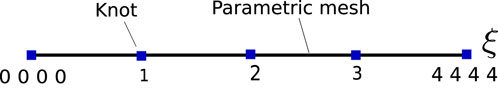
Figure 1. The one-dimensional parametric space for a knot vector.

The B-spline basis functions for a particular knot vector are expressed using the Cox-de Boor recursion formula. For $p=0$, we have Eq. 2. And we have Eq. 3 for $p\ge 1$.

$N_{a,0}\left(\xi \right)=\left\{\begin{array}{cc}\hfill & 1\mathrm{i}\mathrm{f}{\xi }_a\le \xi <{\xi }_{a+1},\hfill \\ \hfill & 0\mathrm{o}\mathrm{t}\mathrm{h}\mathrm{e}\mathrm{r}\mathrm{w}\mathrm{i}\mathrm{s}\mathrm{e},\hfill \end{array}\right.(2)$

$N_{a,p}\left(\xi \right)=\frac{\xi -{\xi }_a}{{\xi }_{a+p}-{\xi }_a}{N}_{a,p-1}\left(\xi \right)+\frac{{\xi }_{a+p+1}-\xi }{{\xi }_{a+p+1}-{\xi }_{a+1}}{N}_{a+1,p-1}\left(\xi \right).(3)$

B-spline basis functions are well-suited for numerical analysis due to their many beneficial properties, such as linear independence. The B-spline curve may be produced by linearly mixing B-spline basis functions and control points, as shown in Eq. 4.

$\mathbf{x}\left(\xi \right)={\displaystyle \sum _{i=1}^n}{N}_{a,p}\left(\xi \right){\mathbf{P}}_{a,p},(4)$

where x is the B-spline curve, and the coefficient P_a,p denotes the coordinates of the control point. This means that the basis function of a B-spline curve is the translation of a parametric one-dimensional space into real space. The following two-dimensional parametric spaces have a knot vector in each dimension, as shown in Eqs 5, 6.

$\left[{\xi }_1,{\xi }_2,\dots ,{\xi }_{n+p+1}\right],{\xi }_a\in \mathbb{R},(5)$

$\left[{\eta }_1,{\eta }_2,\dots ,{\eta }_{m+l+1}\right],{\xi }_b\in \mathbb{R}.(6)$

The B-spline surface may be constructed using the tensor product property, as shown in Eq. 7.

$\mathbf{x}\left(\xi ,\eta \right)={\displaystyle \sum _{a=1}^n}{\displaystyle \sum _{b=1}^m}{N}_{a,p}\left(\xi \right)N_{b,l}\left(\eta \right){\mathbf{P}}_{a,b},(7)$

where the matching number of the basis function in each dimension is denoted by n and m. It should be noted that the lack of the Kronecker delta characteristic means that B-spline control points are typically not on the surface.

NURBS is used to expand B-splines by associating a weight coefficient with each control point. With NURBS, designers may accurately represent a variety of curves with conic segments, such as circles and ellipses, and increase control over the curves without increasing the number or degree of control points. Eqs 8, 9 represent the B-spline basis functions in two dimensions, from which the NURBS basis functions are generated.

$R_{a,b}\left(\xi ,\eta \right)=\frac{N_{b,p}\left(\xi \right)N_{b,l}\left(\eta \right)w_{a,b}}{W\left(\xi ,\eta \right)},(8)$

$W\left(\xi ,\eta \right)={\displaystyle \sum _{a=1}^n}{\displaystyle \sum _{b=1}^m}{N}_{a,p}\left(\xi \right)N_{b,l}\left(\eta \right)w_{a,b}.(9)$

in which w is the weight coefficient.

NURBS surfaces are defined using NURBS basis functions and control points, as shown in Eq. 10, in a manner akin to that of B-spline surfaces. We may recast Eq. 10 as Eq. 11 by utilizing the global index A to iterate between basis functions or control points.

$\mathbf{x}\left(\xi ,\eta \right)={\displaystyle \sum _{a=1}^n}{\displaystyle \sum _{b=1}^m}{R}_{a,p}\left(\xi \right)R_{b,l}\left(\eta \right){\mathbf{P}}_{a,b}.(10)$

$\mathbf{x}\left(\xi ,\eta \right)={\displaystyle \sum _{A=1}^{N_A}}{R}_A\left(\xi ,\eta \right){\mathbf{P}}_A.(11)$

The knot insertion operator can be used to add more control points without changing the structural shape. This feature contributes to improving the accuracy of predicting physical fields while preserving geometric correctness by using the h-refinement approach.

3 Derivation of structural-acoustic interaction analysis

3.1 Derivation of boundary element method

The time-harmonic wave field of sound in the Helmholtz equation is described by Eq. 12.

${\mathit{\nabla }}^{2}p\left(x\right)+k^{2}p\left(x\right)=0,(12)$

in which the wave number is k and the sound pressure is p.

A boundary integral equation unique to the structural boundary Γ may be constructed from Eq. 12 to Eq. 13.

$c\left(x\right)p\left(x\right)+{\int }_{\mathrm{\Gamma }}F\left(x,y\right)p\left(y\right)\mathit{d}\mathrm{\Gamma }\left(y\right)={\int }_{\mathrm{\Gamma }}G\left(x,y\right)q\left(y\right)d\mathrm{\Gamma }\left(y\right),x,y\in \mathrm{\Gamma },(13)$

where the source point is x, the field point is y, the Green’s function is G (x, y), the intensity of the incoming wave is p, the normal derivative of p is q, q(y) = iρωv(y), the structure material’s density is ρ, the frequency of incoming wave is ω, the normal velocity is v, and the normal derivative of G is F. If the boundary Γ is smooth near the source point x, then c(x) = 1/2.

In three-dimensional situations, the Green’s function G (x, y) may be expressed using Eq. 14 for acoustic concerns.

$G\left(x,y\right)=\frac{e^{ikr}}{4\pi r},(14)$

in which $r=\left|y-x\right|$ is the distance between x and y.

The derivative of the integral representation in Eq. 13 with respect to the outer normal at point x may be represented as Eq. 15 in situations when the source point x has a smooth border Γ.

$\frac{1}{2}q\left(x\right)+{\int }_{\mathrm{\Gamma }}\frac{\partial F\left(x,y\right)}{\partial n\left(x\right)}p\left(y\right)d\mathrm{\Gamma }\left(y\right)={\int }_{\mathrm{\Gamma }}\frac{\partial G\left(x,y\right)}{\partial n\left(x\right)}q\left(y\right)d\mathrm{\Gamma }\left(y\right).(15)$

It is generally known that applying a single Helmholtz boundary integral equation to issues needing external boundary values is challenging due to nonuniqueness. The nonuniqueness problem is effectively handled in this work by utilizing the Burton-Miller technique Burton and Miller [57], which combines the linear Eqs 13, 15. The singular boundary integrals caused by Eqs 13, 15 may also be directly and effectively computed using the Cauchy principal value and the Hadamard finite part integral technique Zheng et al. [22].

One can get the system of linear algebraic equations represented in Eq. 16, if the border Γ is split up into elements by combining all of the center-of-element collocation point equations and displaying them using matrix representations Ciskowski and Brebbia [58].

$\mathbf{H}\mathbf{p}=\mathbf{G}\mathbf{q}+{\mathbf{p}}_{\mathbf{i}},(16)$

in which the coefficient matrices are H and G, the nodal pressure caused by the incoming wave is p_i.

3.2 Derivation of finite element method

This section contains expressions related to the structural-acoustic analysis as described in detail by researchers Fritze et al. [6]; Chen et al. [59]. The steady-state reaction of the structure may be deduced from the frequency-response analysis if it is subjected to a harmonic load. Eq. 17 derives the linear system of the structural-acoustic equation.

$\begin{array}{cc}\hfill \left(\mathbf{K}+\mathrm{i}\omega \mathbf{C}-{\omega }^2\mathbf{M}\right)\mathbf{u}\left(\omega \right)& =\mathbf{A}\mathbf{u}=\mathbf{f},\hfill \\ \hfill \mathbf{A}& =\mathbf{K}+\mathrm{i}\omega \mathbf{C}-{\omega }^2\mathbf{M},\hfill \end{array}(17)$

where the stiffness matrix is K, the damping matrix is C, the mass matrix is M, the nodal displacement vector is u, the imaginary unit is $\mathrm{i}=\sqrt{-1}$, the excitation frequency is ω, and the complete excitation is f.

It should be noted that damping may result in a noticeable phase angle in the steady-state response, even though it keeps the same frequency with the applied load. If the load is not harmonic, Eq. 17 can still be applied by decomposing the time-dependent impulses into the frequency domain. In order to take into account the effects of the acoustic pressure applied to structural surfaces on various aspects, a coupling matrix is included to move the structural nodal load from the fluid effect to fluid nodal pressure. Eq. 18 might thus be used to define the whole excitation, which combines the structural load and the acoustic load.

$\begin{array}{cc}\hfill \mathbf{A}\mathbf{u}& ={\mathbf{C}}_{\mathbf{s}\mathbf{f}}\mathbf{p}+{\mathbf{f}}_{\mathbf{s}}=\mathbf{f},\hfill \\ {\mathbf{C}}_{\mathbf{sf}}& ={\int }_{{\mathrm{\Gamma }}_{\mathit{int}}}{\mathbf{N}}_{\mathbf{s}}^{\mathbf{T}}\mathbf{n}{\mathbf{N}}_{\mathbf{f}}d\mathrm{\Gamma },\hfill \end{array}(18)$

where N_s is the interpolation function in structure, n is the structural surface’s outward normal direction, N_f is the interpolation function in fluid, Γ is the interaction surface, C_sf is the coupling matrix, p is the fluid nodal pressure, and f_s is the structural load.

The structural nodal load is directed from the fluid effect to the fluid nodal pressure via the coupling matrix C_sf. The nodal displacement may then be determined using Eq. 19.

$\mathbf{u}={\mathbf{A}}^{-1}\mathbf{f}.(19)$

3.3 Derivation of FEM/BEM interaction analysis

The exact formulae for FEM/BEM modeling were published by Fritze et al. [6], and this section contains related equations. The continuity constraint over the interaction surface connects the governing equations from the previous section, as shown in Eq. 20. Next, it makes sense to express the normal velocity v as a function of the displacement u, in line with Eq. 21.

$\mathbf{q}=-\mathrm{i}\omega \rho \mathbf{v},(20)$

$\begin{array}{c}\mathbf{v}=\mathrm{i}\omega {\mathbf{S}}^{-\mathbf{1}}{\mathbf{C}}_{\mathbf{fs}}\mathbf{u},\hfill \\ \mathbf{S}={\int }_{{\mathrm{\Gamma }}_{\mathit{int}}}{\mathbf{N}}_{\mathbf{f}}^{\mathbf{T}}{\mathbf{N}}_{\mathbf{f}}d\mathrm{\Gamma },\hfill \\ {\mathbf{C}}_{\mathbf{fs}}={\mathbf{C}}_{\mathbf{s}\mathbf{f}}^{\mathbf{T}}.\hfill \end{array}(21)$

We can get Eq. 22 by combining Eqs 16, 20, 21. Eqs 17, 22 may be combined to form an equation system, as demonstrated in Eq. 23.

$\mathbf{H}\mathbf{p}={\omega }^2\rho \mathbf{G}{\mathbf{S}}^{-\mathbf{1}}{\mathbf{C}}_{\mathbf{f}\mathbf{s}}\mathbf{u}+{\mathbf{p}}_{\mathbf{i}}.(22)$

$\left[\begin{array}{cc}\hfill \mathbf{A}\hfill & \hfill -{\mathbf{C}}_{\mathbf{sf}}\hfill \\ \hfill -{\omega }^2\rho \mathbf{G}{\mathbf{S}}^{-\mathbf{1}}{\mathbf{C}}_{\mathbf{f}\mathbf{s}}\hfill & \hfill \mathbf{H}\hfill \end{array}\right]\left\{\begin{array}{c}\hfill \mathbf{u}\hfill \\ \hfill \mathbf{p}\hfill \end{array}\right\}=\left\{\begin{array}{c}\hfill {\mathbf{f}}_{\mathbf{s}}\hfill \\ \hfill {\mathbf{p}}_{\mathbf{i}}\hfill \end{array}\right\}.(23)$

Since the direct iterations on Eq. 23 converge slowly, solving the system equation directly would need a lot more computing power and storage. Moreover, obtaining extremely accurate numerical findings is challenging. We present the following technique for solving the aforementioned non-symmetric linear system without the need for an iterative solution. It is possible to get the coupled boundary element equation Fritze et al. [6] by replacing Eq. 19 in Eq. 22, as shown in Eq. 24. The solution of the linear equations in Eq. 24 may be performed using a sparse direct solver. To speed up the solution, FMM and the Generalized Minimum Residual (GMRES) iterative solver are used.

$\begin{array}{c}\mathbf{H}\mathbf{p}-\mathbf{G}\mathbf{W}{\mathbf{C}}_{\mathbf{s}\mathbf{f}}\mathbf{p}={\mathbf{G}\mathbf{W}\mathbf{f}}_{\mathbf{s}}+{\mathbf{p}}_{\mathbf{i}},\hfill \\ \hfill \mathbf{W}={\omega }^2\rho {\mathbf{S}}^{-\mathbf{1}}{\mathbf{C}}_{\mathbf{f}\mathbf{s}}{\mathbf{A}}^{-\mathbf{1}}.\end{array}(24)$

4 Derivation of sensitivity analysis in shape design

The goal of shape optimization is to identify, within predetermined bounds, the ideal design parameters that characterize the intended form of the given structure. Gradients of given cost functions can be found by applying shape design sensitivity analysis. The obtained gradients may then be used to select which way to search for the optimal ranges of the design variables. Therefore, the acoustic shape sensitivity research Zheng et al. [22]; Chen et al. [60] is frequently the first and most important phase in the process of creating and optimizing acoustic shapes. The chain rule of differentiation is used in the direct approach to compute the sensitivity of the function after determining the sensitivity of the variables. Because this method is so intimately associated with the analytical process, it is quite successful.

Eq. 25 can be generated by differentiating Eq. 17 with respect to the design variable in the shape design sensitivity computation using FEM.

$\left(\dot{\mathbf{K}}+i\omega \dot{\mathbf{C}}-{\omega }^2\dot{\mathbf{M}}\right)\mathbf{u}+\left(\mathbf{K}+i\omega \mathbf{C}-{\omega }^2\mathbf{M}\right)\dot{\mathbf{u}}=\dot{\mathbf{A}}\mathbf{u}+\mathbf{A}\dot{\mathbf{u}}.(25)$

To get Eqs. 13, 15, 26, 27, are differentiated with respect to the design variable in the case when the source point x is surrounded by a smooth border Γ.

$\begin{array}{ll}\hfill \frac{1}{2}\dot{p}\left(x\right)& ={\int }_{\mathrm{\Gamma }}\left[\dot{G}\left(x,y\right)q\left(y\right)-\dot{F}\left(x,y\right)p\left(y\right)\right]d\mathrm{\Gamma }\left(y\right)\hfill \\ \hfill & +{\int }_{\mathrm{\Gamma }}\left[G\left(x,y\right)\dot{q}\left(y\right)-F\left(x,y\right)\dot{p}\left(y\right)\right]d\mathrm{\Gamma }\left(y\right)\hfill \\ \hfill & +{\int }_{\mathrm{\Gamma }}\left[G\left(x,y\right)q\left(y\right)-F\left(x,y\right)p\left(y\right)\right]d\dot{\mathrm{\Gamma }}\left(y\right).\hfill \end{array}(26)$

$\begin{array}{ll}\hfill \frac{1}{2}\dot{q}\left(x\right)& ={\int }_{\mathrm{\Gamma }}\left[\dot{\frac{\partial G\left(x,y\right)}{\partial n\left(x\right)}}q\left(y\right)-\dot{\frac{\partial F\left(x,y\right)}{\partial n\left(x\right)}}p\left(y\right)\right]d\mathrm{\Gamma }\left(y\right)\hfill \\ \hfill & +{\int }_{\mathrm{\Gamma }}\left[\frac{\partial G\left(x,y\right)}{\partial n\left(x\right)}\dot{q}\left(y\right)-\frac{\partial F\left(x,y\right)}{\partial n\left(x\right)}\dot{p}\left(y\right)\right]d\mathrm{\Gamma }\left(y\right)\hfill \\ \hfill & +{\int }_{\mathrm{\Gamma }}\left[\frac{\partial G\left(x,y\right)}{\partial n\left(x\right)}q\left(y\right)-\frac{\partial F\left(x,y\right)}{\partial n\left(x\right)}p\left(y\right)\right]d\dot{\mathrm{\Gamma }}\left(y\right).\hfill \end{array}(27)$

For three-dimensional problems, we have Eq. 28

$\begin{array}{c}\hfill \dot{G}\left(x,y\right)=-\frac{e^{ikr}}{4\pi r^2}\left(1-ikr\right)\frac{\partial r}{\partial y_i}\left({\dot{y}}_i-{\dot{x}}_i\right),\\ \dot{F}\left(x,y\right)=\frac{e^{ikr}}{4\pi r^3}\left[\left(3-3ikr-k^2{r}^2\right)\frac{\partial r}{\partial n\left(y\right)}\frac{\partial r}{\partial y_j}-\left(1-ikr\right)n_j\left(y\right)\right]\left({\dot{y}}_j-{\dot{x}}_j\right)\\ -\frac{e^{ikr}}{4\pi r^2}\left(1-ikr\right)\frac{\partial r}{\partial y_i}{\dot{n}}_i\left(y\right),\hfill \\ \hfill \dot{r}=r_{,j}\left({\dot{y}}_j-{\dot{x}}_j\right).\end{array}(28)$

The singular boundary integrals introduced by Eqs 26, 27 may be computed directly and efficiently using the Cauchy principal value and the Hadamard finite part integral technique Zheng et al. [22].

Applying Eq. 22 and differentiating Eq. 24 with respect to the design variable will result in Eq. 29 for the sensitivity analysis for shape design using coupling FEM/BEM. Since the matrices are full and asymmetric, solving Eq. 29 directly with normal BEM requires a significant amount of computational work. FMM and GMRES, on the other hand, can be utilized to speed up computation. Eqs 24, 29 use FMM to accelerate the matrix-vector combinations. GMRES is used to solve the associated sensitivity equation and the formula for the FEM/BEM coupling.

$\begin{array}{c}\hfill \mathbf{H}\dot{\mathbf{p}}-\mathbf{G}\mathbf{W}{\mathbf{C}}_{\mathbf{s}\mathbf{f}}\dot{\mathbf{p}}=\dot{\mathbf{G}}\mathbf{X}+\mathbf{G}\mathbf{Y}-\dot{\mathbf{H}}\mathbf{p},\\ \hfill \mathbf{X}=\mathbf{W}\left({\mathbf{C}}_{\mathbf{s}\mathbf{f}}\mathbf{p}+{\mathbf{f}}_{\mathbf{s}}\right),\\ \hfill \mathbf{Y}=\dot{\mathbf{W}}\left({\mathbf{C}}_{\mathbf{s}\mathbf{f}}\mathbf{p}+{\mathbf{f}}_{\mathbf{s}}\right)+\mathbf{W}\left(\dot{{\mathbf{C}}_{\mathbf{s}\mathbf{f}}}\mathbf{p}+\dot{{\mathbf{f}}_{\mathbf{s}}}\right),\\ \dot{\mathbf{W}}={\omega }^2\rho \left(\dot{{\mathbf{S}}^{-\mathbf{1}}}{\mathbf{C}}_{\mathbf{f}\mathbf{s}}{\mathbf{A}}^{-\mathbf{1}}+{\mathbf{S}}^{-\mathbf{1}}\dot{{\mathbf{C}}_{\mathbf{f}\mathbf{s}}}{\mathbf{A}}^{-\mathbf{1}}+{\mathbf{S}}^{-\mathbf{1}}{\mathbf{C}}_{\mathbf{f}\mathbf{s}}\dot{{\mathbf{A}}^{-\mathbf{1}}}\right).\end{array}(29)$

5 Numerical examples

In this part, numerical examples for real-world engineering problems illustrate the effectiveness of the proposed method. The method for doing the numerical analysis is built using our in-house Fortran code.

5.1 Spherical shell model

This subsection makes use of Figure 2’s concept of a thin underwater spherical shell exposed to plane wave incidence. With an amplitude of 1, the plane wave is incident in the x-direction. The sound pressure and sensitivity at point (3, 0, 0) are examined, and the coordinate origin (0, 0, 0) is located in the center of the spherical shell. The radius of the spherical shell is r = 0.9 m and the shell thickness is t = 0.009 m. Water has a density of ρ_f = 1.0 × 10³ kg/m³, and sound waves travel at a speed of c = 1,482 m/s in this fluid.

Figure 2

Figure 2. Diagram of the spherical shell model with incoming wave.

For the model in Figure 2, the sound pressure values at the point (3, 0, 0) are analyzed. Figure 3 gives the numerical and analytical results of the sound pressure. The GMRES implementation uses the FMM approach to accelerate the linear solution. The considerable agreement between the analytical and numerical results in Figure 3 indicates that the FMM approach maintains the extraordinary accuracy of the conventional BEM.

Figure 3

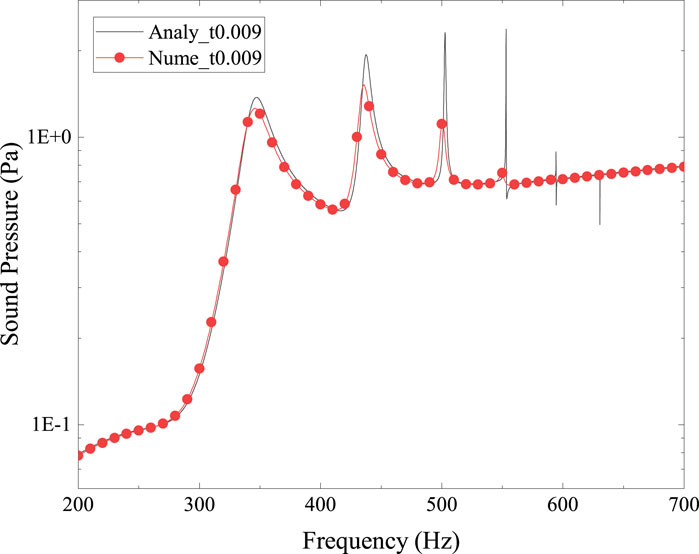
Figure 3. Sound pressure at location (3, 0, 0) for spherical shell model, numerical result vs. analytical result. The radius r = 0.9 m, shell thichness t = 0.009 m.

Sensitivity analysis plays a crucial role in shape optimization. In this example, the objective function is the sound pressure at position (3,0,0), the design variable is the spherical shell’s thickness t. Figure 4 displays the sound pressure sensitivity. As can be seen from Figure 4, the numerical solution agrees well with the analytical solution. In addition, Figures 3, 4 show how both sound pressure and sensitivity increase significantly at peak resonance. Furthermore, in Figure 4, the location of the sharp increase in sound pressure sensitivity does not always correspond to the resonance peak in Figure 3. At computed frequencies where the sound pressure curve is generally flat, there may also be a significant sensitivity to sound pressure. This highlights how crucial it is to investigate sound pressure and sensitivity within a frequency range.

Figure 4

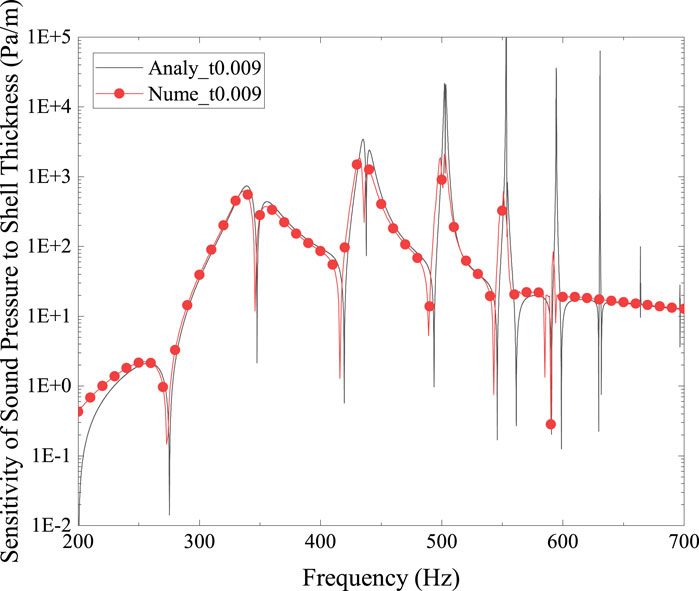
Figure 4. Sensitivity of sound pressure to shell thickness at location (3, 0, 0) for spherical shell model, numerical result vs. analytical result. The radius r = 0.9 m, shell thichness t = 0.009 m.

The sound pressure on the boundary surface of the spherical shell at 300 Hz, 500 Hz, and 700 Hz frequencies is depicted in Figure 5. The x − y and x − z planes exhibit symmetrical feature in these figures, while the sound pressure exhibits a phase difference along the x-axis. These results make sense as the plane wave happens along the x-axis.

Figure 5

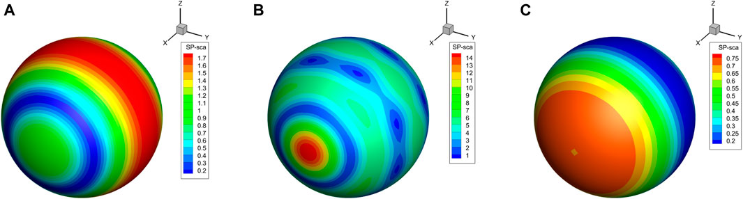
Figure 5. (A) Sound pressure on the spherical shell surface at frequency of 300 Hz. (B) Sound pressure on the spherical shell surface at frequency of 500 Hz. (C) Sound pressure on the spherical shell surface at frequency of 700 Hz. Sound pressure at frequencies of 300 Hz, 500 Hz, and 700 Hz on the spherical shell surface. The radius r = 0.9 m, shell thichness t = 0.009 m.

5.2 Diesel engine box model

In this section, a simplified diesel engine box shell model (as shown in Figure 6) is used for sound field analysis under the action of incident waves. As in Section 5.1, the plane wave is incident along the x-direction with an amplitude of 1. Water is the fluid. The model is located within the coordinate range where x ∈ [−0.5, 0.48], y ∈ [−0.2, 0.2], and z ∈ [0, 0.69]. The thickness of the shell is 0.01 m. Analysis is done on the sound pressure and sensitivity at positions (1, 0, 0), (5, 0, 0), and (10, 0, 0).

Figure 6

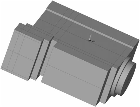
Figure 6. Diagram of the diesel engine box model.

Figure 7 shows the sound pressure at positions (1, 0, 0), (5, 0, 0), and (10, 0, 0), while Figure 8 shows how sensitive the sound pressure is to shell thickness at the same places.

Figure 7

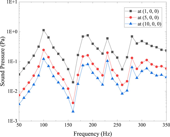
Figure 7. Sound pressure at location (1, 0, 0), (5, 0, 0) and (10, 0, 0) for diesel engine box model. The shell thichness t = 0.01 m.

Figure 8

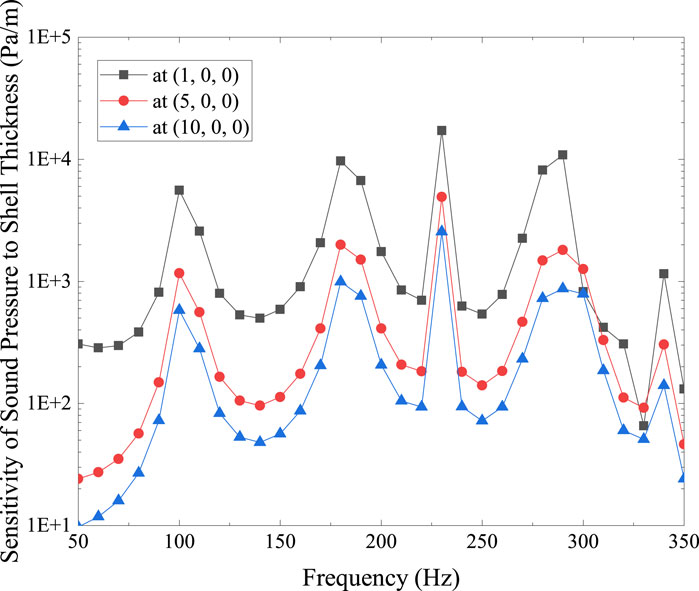
Figure 8. Sensitivity of sound pressure to shell thickness at location (1, 0, 0), (5, 0, 0) and (10, 0, 0) for diesel engine box model. The shell thichness t = 0.01 m.

The sound pressure trend at various calculation locations in relation to the computation frequency is similar in Figure 7. The diesel engine model’s eigenfrequency is where the peak is located. For various calculation sites, the sensitivity of sound pressure to shell thickness is shown in Figure 8 in a similar trend. The peaks on both sides emerge at comparable computational frequency when comparing Figures 7, 8. Take note that the sensitivity in Figure 8 peaks at 340 Hz, while Figure 7 does not show this peak. As was concluded in Section 5.1, at computed frequencies where the sound pressure is rather flat, it is possible to have substantial sound pressure sensitivity. This emphasizes once more how crucial it is to examine sound pressure and sensitivity over a band of frequencies. Furthermore, in Figures 7, 8, the sound pressure and its sensitivity decrease as the distance between the model and the computation point increases [computation point from (1, 0, 0) to (10, 0, 0)]. This result is reasonable considering the attenuation of energy.

The sound pressure on the model’s boundary surface in Figure 6 is displayed in Figure 9 at the frequency of 100 Hz, 200 Hz, and 300 Hz. As seen by Figure 9, the sound pressure peaks on the diesel engine model’s surface often emerge on both sides of the structure when stimulated by a plane incident wave in the x-direction. Additionally, when the computational frequency exceeds a certain threshold, (e.g., 300 Hz), the acoustic pressure peak appears on the plane that meets the incident wave. This phenomena may be investigated in greater detail for various material properties, geometrical factors, and incident wave frequencies in further studies.

Figure 9

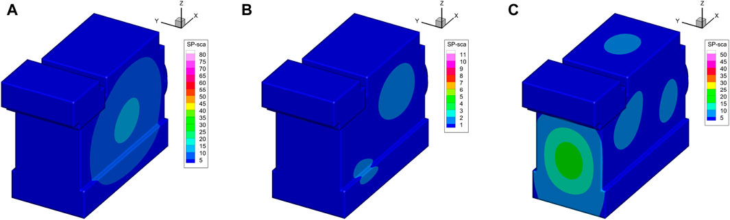
Figure 9. (A) Sound pressure on the diesel engine’s surface at frequency of 100 Hz (B) Sound pressure on the diesel engine’s surface at frequency of 200 Hz. (C) Sound pressure on the diesel engine’s surface at frequency of 300 Hz. Sound pressure at frequencies of 100 Hz, 200 Hz, and 300 Hz on the diesel engine’s surface. The thichness t = 0.01 m.

The fluid effect must be taken into account while studying the vibro-acoustic coupling problem for thin-shell designs, as the numerical simulations unequivocally demonstrate. Consequently, the coupling analysis must be performed. Since the mesh quality directly affects the computational accuracy of the coupling analysis, defining high-quality meshes is essential. This indicates that both engineering and academics stand to gain much from the use of IGA, such as NURBS, to improve computational accuracy.

6 Conclusion

Utilizing a coupling approach based on BEM and FEM, sensitivity analysis and the modeling of the acoustic-structure coupling are completed. FEM is used to simulate the problem’s structural components. The boundary of the structure under study, which is also the boundary of the acoustic domain, is discretized using BEM in order to obviate the need to mesh the acoustic space. FMM is used to accelerate the matrix-vector output. By eliminating the need for meshing and utilizing CAD models to directly examine the sensitivity of the structural-acoustic interaction, NURBS IGABEM eliminates geometric errors. Sound pressure sensitivity equations are developed for connecting structural-acoustic systems. To illustrate the precision and usefulness of the suggested approach, numerical examples are shown. The suggested technique might be used to quantitatively estimate the effect of design features on the sound field in real-world circumstances.

Data availability statement

The original contributions presented in the study are included in the article/Supplementary material, further inquiries can be directed to the corresponding author.

Author contributions

YX: Conceptualization, Investigation, Methodology, Project administration, Resources, Software, Supervision, Writing–original draft. SY: Data curation, Formal Analysis, Funding acquisition, Validation, Visualization, Writing–review and editing.

Funding

The author(s) declare that financial support was received for the research, authorship, and/or publication of this article. Sponsored by the Henan Provincial Key R&D and Promotion Project under Grant No. 232102220033, the Zhumadian 2023 Major Science and Technology Special Project under Grant No. ZMDSZDZX2023002, the Natural Science Foundation of Henan under Grant No. 222300420498, and the Postgraduate Education Reform and Quality Improvement Project of Henan Province under Grant No. YJS2023JD52.

Conflict of interest

The authors declare that the research was conducted in the absence of any commercial or financial relationships that could be construed as a potential conflict of interest.

Publisher’s note

All claims expressed in this article are solely those of the authors and do not necessarily represent those of their affiliated organizations, or those of the publisher, the editors and the reviewers. Any product that may be evaluated in this article, or claim that may be made by its manufacturer, is not guaranteed or endorsed by the publisher.

References

1. Junger MC, Feit D. Sound, structures, and their interaction, 225. MA: MIT press Cambridge (1986).

Google Scholar

2. Sommerfeld A. Partial differential equations in Physics. Academic Press (1949). doi:10.1016/B978-0-12-654658-3.50003-3

CrossRef Full Text | Google Scholar

3. Engleder OSS. Stabilized boundary element methods for exterior Helmholtz problems. Numerische Mathematik (2008) 110:145–60. doi:10.1007/s00211-008-0161-y

CrossRef Full Text | Google Scholar

4. Chen L, Zhang Y, Lian H, Atroshchenko E, Ding C, Bordas S. Seamless integration of computer-aided geometric modeling and acoustic simulation: isogeometric boundary element methods based on catmull-clark subdivision surfaces. Adv Eng Softw (2020) 149:102879. doi:10.1016/j.advengsoft.2020.102879

CrossRef Full Text | Google Scholar

5. Everstine GC, Henderson FM. Coupled finite element/boundary element approach for fluid-structure interaction. The J Acoust Soc America (1990) 87:1938–47. doi:10.1121/1.399320

CrossRef Full Text | Google Scholar

6. Fritze D, Marburg S, Hardtke HJ. FEM-BEM-coupling and structural-acoustic sensitivity analysis for shell geometries. Comput Structures (2005) 83:143–54. doi:10.1016/j.compstruc.2004.05.019

CrossRef Full Text | Google Scholar

7. Chen L, Cheng R, Li S, Lian H, Zheng C, Bordas S. A sample-efficient deep learning method for multivariate uncertainty qualification of acoustic-vibration interaction problems. Comput Methods Appl Mech Eng (2022) 393:114784. doi:10.1016/j.cma.2022.114784

CrossRef Full Text | Google Scholar

8. Martinsson P, Rokhlin V. A fast direct solver for boundary integral equations in two dimensions. J Comput Phys (2005) 205:1–23. doi:10.1016/j.jcp.2004.10.033

CrossRef Full Text | Google Scholar

9. Martinsson P, Rokhlin V. A fast direct solver for scattering problems involving elongated structures. J Comput Phys (2007) 221:288–302. doi:10.1016/j.jcp.2006.06.037

CrossRef Full Text | Google Scholar

10. Bebendorf SMR. Adaptive low-rank approximation of collocation matrices. Computing (2003) 70:1–24. doi:10.1007/s00607-002-1469-6

CrossRef Full Text | Google Scholar

11. Greengard L, Rokhlin V. A fast algorithm for particle simulations. J Comput Phys (1987) 73:325–48. doi:10.1016/0021-9991(87)90140-9

CrossRef Full Text | Google Scholar

12. Coifman R, Rokhlin V, Wandzura S. The fast multipole method for the wave equation: a pedestrian prescription. IEEE Antennas Propagation Mag (1993) 35:7–12. doi:10.1109/74.250128

CrossRef Full Text | Google Scholar

13. Rokhlin V. Diagonal forms of translation operators for the Helmholtz equation in three dimensions. Appl Comput Harmonic Anal (1993) 1:82–93. doi:10.1006/acha.1993.1006

CrossRef Full Text | Google Scholar

14. Schneider S. FE/FMBE coupling to model fluid-structure interaction. Int J Numer Methods Eng (2008) 76:2137–56. doi:10.1002/nme.2399

CrossRef Full Text | Google Scholar

15. Kim NH, Dong J. Shape sensitivity analysis of sequential structural-acoustic problems using FEM and BEM. J Sound Vibration (2006) 290:192–208. doi:10.1016/j.jsv.2005.03.013

CrossRef Full Text | Google Scholar

16. Chen L, Zhao J, Lian H, Yu B, Atroshchenko E, Li P. A BEM broadband topology optimization strategy based on Taylor expansion and SOAR method-Application to 2D acoustic scattering problems. Int J Numer Methods Eng (2023) 124:5151–82. doi:10.1002/nme.7345

CrossRef Full Text | Google Scholar

17. Qu Y, Zhou Z, Chen L, Lian H, Li X, Hu Z, et al. Uncertainty quantification of vibro-acoustic coupling problems for robotic manta ray models based on deep learning. Ocean Eng (2024) 299:117388. doi:10.1016/j.oceaneng.2024.117388

CrossRef Full Text | Google Scholar

18. Marburg S. Developments in structural-acoustic optimization for passive noise control. Arch Comput Methods Eng (2002) 9:291–370. doi:10.1007/BF03041465

CrossRef Full Text | Google Scholar

19. Lamancusa J. Numerical optimization techniques for structural-acoustic design of rectangular panels. Comput Structures (1993) 48:661–75. doi:10.1016/0045-7949(93)90260-K

CrossRef Full Text | Google Scholar

20. Hambric SA. Sensitivity calculations for broad-band acoustic radiated noise design optimization problems. J Vibration Acoust (1996) 118:529–32. doi:10.1115/1.2888219

CrossRef Full Text | Google Scholar

21. Marburg S, Hardtke HJ. Shape optimization of a vehicle hat-shelf: improving acoustic properties for different load cases by maximizing first eigenfrequency. Comput Structures (2001) 79:1943–57. doi:10.1016/S0045-7949(01)00107-9

CrossRef Full Text | Google Scholar

22. Zheng C, Matsumoto T, Takahashi T, Chen H. Explicit evaluation of hypersingular boundary integral equations for acoustic sensitivity analysis based on direct differentiation method. Eng Anal Boundary Elem (2011) 35:1225–35. doi:10.1016/j.enganabound.2011.05.004

CrossRef Full Text | Google Scholar

23. Liu Z, Bian P, Qu Y, Huang W, Chen L, Chen J, et al. A galerkin approach for analysing coupling effects in the piezoelectric semiconducting beams. Eur J Mechanics-A/Solids (2024) 103:105145. doi:10.1016/j.euromechsol.2023.105145

CrossRef Full Text | Google Scholar

24. Choi K, Shim I, Wang S. Design sensitivity analysis of structure-induced noise and vibration. J Vibration Acoust (1997) 119:173–9. doi:10.1115/1.2889699

CrossRef Full Text | Google Scholar

25. Wang S. Design sensitivity analysis of noise, vibration, and harshness of vehicle body structure. Mech Structures Machines (1999) 27:317–35. doi:10.1080/08905459908915701

CrossRef Full Text | Google Scholar

26. Hughes T, Cottrell J, Bazilevs Y. Isogeometric analysis: CAD, finite elements, NURBS, exact geometry and mesh refinement. Comput Methods Appl Mech Eng (2005) 194:4135–95. doi:10.1016/j.cma.2004.10.008

CrossRef Full Text | Google Scholar

27. Chen L, Lu C, Lian H, Liu Z, Zhao W, Li S, et al. Acoustic topology optimization of sound absorbing materials directly from subdivision surfaces with isogeometric boundary element methods. Comput Methods Appl Mech Eng (2020) 362:112806. doi:10.1016/j.cma.2019.112806

CrossRef Full Text | Google Scholar

28. Shen X, Du C, Jiang S, Sun L, Chen L. Enhancing deep neural networks for multivariate uncertainty analysis of cracked structures by POD-RBF. Theor Appl Fracture Mech (2023) 125:103925. doi:10.1016/j.tafmec.2023.103925

CrossRef Full Text | Google Scholar

29. Simpson R, Bordas S, Trevelyan J, Rabczuk T. A two-dimensional isogeometric boundary element method for elastostatic analysis. Comput Methods Appl Mech Eng (2012) 209-212:87–100. doi:10.1016/j.cma.2011.08.008

CrossRef Full Text | Google Scholar

30. Simpson R, Bordas S, Lian H, Trevelyan J. An isogeometric boundary element method for elastostatic analysis: 2D implementation aspects. Comput Structures (2013) 118:2–12. Special Issue: UK Association for Computational Mechanics in Engineering. doi:10.1016/j.compstruc.2012.12.021

CrossRef Full Text | Google Scholar

31. Scott M, Simpson R, Evans J, Lipton S, Bordas S, Hughes T, et al. Isogeometric boundary element analysis using unstructured T-splines. Comput Methods Appl Mech Eng (2013) 254:197–221. doi:10.1016/j.cma.2012.11.001

CrossRef Full Text | Google Scholar

32. Takahashi T, Matsumoto T. An application of fast multipole method to isogeometric boundary element method for Laplace equation in two dimensions. Eng Anal Boundary Elem (2012) 36:1766–75. doi:10.1016/j.enganabound.2012.06.0042012.06.004

CrossRef Full Text | Google Scholar

33. Zhang S, Yu B, Chen L. Non-iterative reconstruction of time-domain sound pressure and rapid prediction of large-scale sound field based on ig-drbem and pod-rbf. J Sound Vibration (2024) 573:118226. doi:10.1016/j.jsv.2023.118226

CrossRef Full Text | Google Scholar

34. Cao G, Yu B, Chen L, Yao W. Isogeometric dual reciprocity bem for solving non-fourier transient heat transfer problems in fgms with uncertainty analysis. Int J Heat Mass Transfer (2023) 203:123783. doi:10.1016/j.ijheatmasstransfer.2022.123783

CrossRef Full Text | Google Scholar

35. Ginnis A, Kostas K, Politis C, Kaklis P, Belibassakis K, Gerostathis T, et al. Isogeometric boundary-element analysis for the wave-resistance problem using T-splines. Comput Methods Appl Mech Eng (2014) 279:425–39. doi:10.1016/j.cma.2014.07.001

CrossRef Full Text | Google Scholar

36. Chen L, Lian H, Xu Y, Li S, Liu Z, Atroshchenko E, et al. Generalized isogeometric boundary element method for uncertainty analysis of time-harmonic wave propagation in infinite domains. Appl Math Model (2023) 114:360–78. doi:10.1016/j.apm.2022.09.030

CrossRef Full Text | Google Scholar

37. Zhang G, He Z, Qin J, Hong J. Magnetically tunable bandgaps in phononic crystal nanobeams incorporating microstructure and flexoelectric effects. Appl Math Model (2022) 111:554–66. doi:10.1016/j.apm.2022.07.005

CrossRef Full Text | Google Scholar

38. Zhang G, He Z, Gao XL, Zhou H. Band gaps in a periodic electro-elastic composite beam structure incorporating microstructure and flexoelectric effects. Archive Appl Mech (2023) 93:245–60. doi:10.1007/s00419-021-02088-9

CrossRef Full Text | Google Scholar

39. Zhang G, Gao X, Wang S, Hong J. Bandgap and its defect band analysis of flexoelectric effect in phononic crystal plates. Eur J Mechanics-A/Solids (2024) 104:105192. doi:10.1016/j.euromechsol.2023.105192

CrossRef Full Text | Google Scholar

40. Zhang G, He Z, Wang S, Hong J, Cong Y, Gu S. Elastic foundation-introduced defective phononic crystals for tunable energy harvesting. Mech Mater (2024) 191:104909. doi:10.1016/j.mechmat.2024.104909

CrossRef Full Text | Google Scholar

41. Shen X, Du C, Jiang S, Zhang P, Chen L. Multivariate uncertainty analysis of fracture problems through model order reduction accelerated SBFEM. Appl Math Model (2024) 125:218–40. doi:10.1016/j.apm.2023.08.040

CrossRef Full Text | Google Scholar

42. Simpson R, Liu Z, Vázquez R, Evans J. An isogeometric boundary element method for electromagnetic scattering with compatible B-spline discretizations. J Comput Phys (2018) 362:264–89. doi:10.1016/j.jcp.2018.01.025

CrossRef Full Text | Google Scholar

43. Xu Y, Li H, Chen L, Zhao J, Zhang X. Monte Carlo based isogeometric stochastic finite element method for uncertainty quantization in vibration analysis of piezoelectric materials. Mathematics (2022) 10:1840. doi:10.3390/math10111840

CrossRef Full Text | Google Scholar

44. Chen L, Wang Z, Lian H, Ma Y, Meng Z, Li P, et al. Reduced order isogeometric boundary element methods for CAD-integrated shape optimization in electromagnetic scattering. Comput Methods Appl Mech Eng (2024) 419:116654. doi:10.1016/j.cma.2023.116654

CrossRef Full Text | Google Scholar

45. Li H, Chen L, Zhi G, Meng L, Lian H, Liu Z, et al. A direct fe2 method for concurrent multilevel modeling of piezoelectric materials and structures. Comput Methods Appl Mech Eng (2024) 420:116696. doi:10.1016/j.cma.2023.116696

CrossRef Full Text | Google Scholar

46. Qu Y, Pan E, Zhu F, Jin F, Roy A. Modeling thermoelectric effects in piezoelectric semiconductors: new fully coupled mechanisms for mechanically manipulated heat flux and refrigeration. Int J Eng Sci (2023) 182:103775. doi:10.1016/j.ijengsci.2022.103775

CrossRef Full Text | Google Scholar

47. Qu Y, Zhang G, Gao X, Jin F. A new model for thermally induced redistributions of free carriers in centrosymmetric flexoelectric semiconductor beams. Mech Mater (2022) 171:104328. doi:10.1016/j.mechmat.2022.104328

CrossRef Full Text | Google Scholar

48. Qu Y, Jin F, Yang J. Temperature effects on mobile charges in thermopiezoelectric semiconductor plates. Int J Appl Mech (2021) 13:2150037. doi:10.1142/s175882512150037x

CrossRef Full Text | Google Scholar

49. Chen L, Liu C, Zhao W, Liu L. An isogeometric approach of two dimensional acoustic design sensitivity analysis and topology optimization analysis for absorbing material distribution. Comput Methods Appl Mech Eng (2018) 336:507–32. doi:10.1016/j.cma.2018.03.025

CrossRef Full Text | Google Scholar

50. Xu G, Li M, Mourrain B, Rabczuk T, Xu J, Bordas SP. Constructing IGA-suitable planar parameterization from complex CAD boundary by domain partition and global/local optimization. Comput Methods Appl Mech Eng (2018) 328:175–200. doi:10.1016/j.cma.2017.08.052

CrossRef Full Text | Google Scholar

51. Li S, Trevelyan J, Wu Z, Lian H, Wang D, Zhang W. An adaptive SVD-Krylov reduced order model for surrogate based structural shape optimization through isogeometric boundary element method. Comput Methods Appl Mech Eng (2019) 349:312–38. doi:10.1016/j.cma.2019.02.023

CrossRef Full Text | Google Scholar

52. Chen L, Lian H, Liu Z, Chen H, Atroshchenko E, Bordas S. Structural shape optimization of three dimensional acoustic problems with isogeometric boundary element methods. Comput Methods Appl Mech Eng (2019) 355:926–51. doi:10.1016/j.cma.2019.06.012

CrossRef Full Text | Google Scholar

53. Lian H, Chen L, Lin X, Zhao W, Bordas SPA, Zhou M. Noise pollution reduction through a novel optimization procedure in passive control methods. Comput Model Eng Sci (2022) 131:1–18. doi:10.32604/cmes.2022.019705

CrossRef Full Text | Google Scholar

54. Chen L, Lian H, Natarajan S, Zhao W, Chen X, Bordas S. Multi-frequency acoustic topology optimization of sound-absorption materials with isogeometric boundary element methods accelerated by frequency-decoupling and model order reduction techniques. Comput Methods Appl Mech Eng (2022) 395:114997. doi:10.1016/j.cma.2022.114997

CrossRef Full Text | Google Scholar

55. Lu C, Chen L, Luo J, Chen H. Acoustic shape optimization based on isogeometric boundary element method with subdivision surfaces. Eng Anal Boundary Elem (2023) 146:951–65. doi:10.1016/j.enganabound.2022.11.010

CrossRef Full Text | Google Scholar

56. Chen L, Lian H, Dong H, Yu P, Jiang S, Bordas S. Broadband topology optimization of three-dimensional structural-acoustic interaction with reduced order isogeometric fem/bem. J Comput Phys (2024) 509:113051. doi:10.1016/j.jcp.2024.113051

CrossRef Full Text | Google Scholar

57. Burton AJ, Miller GF. The application of integral equation methods to the numerical solution of some exterior boundary-value problems. Proc R Soc Lond (1971) 323:201–10. doi:10.1098/rspa.1971.0097

CrossRef Full Text | Google Scholar

58. Ciskowski RD, Brebbia CA. Boundary element methods in acoustics. Springer (1991).

Google Scholar

59. Chen L, Li H, Guo Y, Chen P, Atroshchenko E, Lian H. Uncertainty quantification of mechanical property of piezoelectric materials based on isogeometric stochastic fem with generalized n th-order perturbation. Eng Comput (2023) 1–21. doi:10.1007/s00366-023-01788-w

CrossRef Full Text | Google Scholar

60. Chen L, Lian H, Liu Z, Gong Y, Zheng C, Bordas S. Bi-material topology optimization for fully coupled structural-acoustic systems with isogeometric FEM-BEM. Eng Anal Boundary Elem (2022) 135:182–95. doi:10.1016/j.enganabound.2021.11.005enganabound.2021.11.005

CrossRef Full Text | Google Scholar