Dialectal tsunamis emerging from the Simmel effect: a statistical approach to the snail-paced spread of cultural epidemic

An attempt is made to settle the controversy on a theory of the concentric distribution of dialectal variants for snails. This theory was presented in 1927 by Kunio Yanagita (1875–1962), outstanding Japanese folklorist. Over more than 95 years, however, its verification remains pending. On the basis of the recent achievement in the linguistic atlas project, time series analysis is made for fitting to the long-tailed rank-frequency relations of cumulative syllabics that are included in the entire dialect sequence of snails. The time reversal asymmetry (TRA) is revealed through comparison between the forward and backward analysis. The validity of the methodology is confirmed through comparison with results for several examples. Computed results show substantial TRAs between the periphery-to-center and center-to-periphery analysis for fitting to the long-tailed distribution in the cumulative frequency versus rank. This feature for the categorial data sequence is consistent with those observed for typical numerical data such as music and heartbeat signals that obey non-Gaussian statistics. Application to the most parsimonious principle yields results being compatible with the above ones, which reproduces the validity of our conclusion. Finally, perturbation analysis is made for several artificially disturbed arrangements of the dialectal strata.

1 Introduction

Since the pioneering work by Jules Gilliéron (1854–1926), who made a voluminous atlas of French dialects, dialect geography has become one of the main areas in linguistics. In North America, a linguistic atlas project (LAP) for mapping variations in American English was started in 1929. Subsequently, until the early years of the present century the project has been continued and eventually realized as the large-scale LAP for English dialects. In Japan a theory on spreading the word denoting a snail in different Japanese dialects (for short, dialectal variant, or dialectal word, for snails) had been presented in 1927 by Kunio Yanagita (1875–1962), along with Kumagusu Minakata (1867–1941) and Shinobu Orikuchi (1887–1953), outstanding Japanese folklorist who was familiar not only with dialectology but also with vast areas about Japanese linguistics and philology. With the theory [1] he insisted on two points: 1) Dialectal words for snails consist of five concentric strata, A to E, as schematically illustrated in Figure 1; and 2) The most archaic variants can be seen in the remotest region from Kyoto, the former capital of Japan. While the former left no room for doubt and was beyond dispute, there was controversy on the validity of the latter. For instance, Haruhiko Kindaichi (1913–2004), a distinguished Japanese linguist, cast doubt upon the Yanagita’s theory, insisting that archaic words are not necessarily found in areas far from the capital [2]. In the long run, however, the controversy over the Yanagita’s hypothesis has been unsettled. Namely, for more than 95 years, to our knowledge, its verification remains pending. Note here that his theory is also applicable to the distribution of dialectal swearwords, for which their propagation velocity was estimated with a model that was constructed on the basis of an Eden growth process [3]. Although their attempt dealt also with the concentric distribution of dialectal words, the aim was focused on how to simulate the spatial dynamics (distance between word fronts versus that from Kyoto), and they did not discuss asymmetries in the propagation. Consequently, it should be put in a context different from our study.

Figure 1

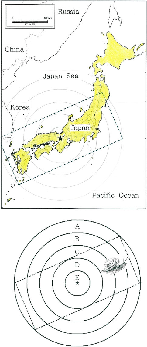
Figure 1. Schematic illustration for the five concentric strata, A to E, of dialectal variants for snails, where the center (star) indicates Kyoto (35°00′N, 135°46′E), a former capital of Japan, and the tilted rectangle enclosed with broken lines represents a truncation of the Japanese Islands [1]. Note that Japanese snails belong to the same genus Euhadra. According to a linguistic atlas that was compiled by the National Institute for Japanese Language, among several dialectal variants such as pumpkins, sweet potatoes, dragonflies, and snails, the distribution of the dialectal variants for snails preserves the distinctest concentricity.

For fashion phenomena, Georg Simmel (1858–1918), a German philosopher as well as sociologist, deeply discussed the sociological mechanism that underlies their propagation [4]. It should be noted that in recent years a fashion wave arising from the imitation, expansion, and decline of baby names has become a fascinating topic as a good example of the cultural epidemic [5–7]. This tendency would once be the case for the old Japan where Kyoto had been the capital for more than a millennium (794–1869). In particular, in the Heian and Muromachi period, the spot had been the kernel of his culture, politics, and economy [3]. With the longing for the urban culture, a very trivial linguistic incident, e.g., something like a collective idiolect for naming snails, might be responsible for sparking off an epidemic, which could be spread by postmen, peddlers, hawkers, and touring theater troupes, as if a ripple emerging from a point source in water spreads concentrically. Depending on circumstances as well as boundary conditions, such a psychological quake might be amplified and eventually developed as if a rising tide or tsunami raises all ships.

In this paper, with the combined use of the Pearson’s regression analysis and the Durbin-Watson statistic for the sequential rank-frequency fit of syllabics in the dialectal data for snails, we aim at settling the long-standing controversy on the Yanagita’s theory of the concentric distribution of dialectal variants for snails. According to the detailed survey by Yanagita for all over the Japanese Islands, there are, respectively, 19, 20, 19, 47, and 29 dialectal variants in the A, B, C, D, and E stratum in Figure 1 [1]. The validity of our statistical method partially owes the recent achievement in the LAP [8–11]. Specifically, time series analysis has been made with fitting to the long-tailed rank-frequency relations of cumulative syllabics that are included in the entire dialectal sequence of snails. Computed results and scattergrams are given in order to examine time reversal asymmetries (TRAs) between the periphery-to-center and center-to-periphery analysis for fitting to the long-tailed distribution in the cumulative frequency versus rank. Subsequently we examine whether this feature for our categorial data sequence is consistent with the TRAs that have been observed for typical numerical data such as music as well as heartbeat signals that obey non-Gaussian statistics [12–15]. Application of the most parsimonious principle that has been developed in the context of phylogenetic data analyses [16–18] is made to explain the significance of our linguistic data. Finally, to make our conclusion firmer, perturbation analysis is made for several artificially disturbed arrangements of the dialectal strata.

2 Methodology

2.1 Japanese syllabary

Along with several European languages such as Spanish, Czech, Serbian, and Greek, as well as a few African ones such as Hausa and Swahili, Japanese has the five-vowel system [19]. According to the literature, this system amounts to 32% in world’s languages [20]. Although the phonological patterns of words in the European languages bear a resemblance to those observed for the loan words of Japanese, the typical feature in the vowel patterns of the Indo-European languages forms a striking contrast to that of the native words of Japanese, where a specific vowel aggregates in a word [21]. Such arrangement of vowels is usually the case with the Ural-Altaic languages showing the vowel harmony, such as Hungarian, Finnish, Turkish, Telugu, and Ainu. Besides, Japanese shares its feature with Malayan, Indonesian, and Polynesian, for which similar syllables are reduplicated. Here it should be noted that these tactics in constructing polysyllabic words will be avoided in major European languages. For instance, in English there are disyllabic words such as “ticktack” and “zigzag,” neither of which becomes “ticktick” nor “zigzig.” In Japanese these are realized as, respectively, kati-kati and kune-kune. Although the reduplication enhances redundancy, in order to achieve reliable transmission of information, the tactics might not necessarily be regarded as disadvantageous [22].

A systematic table of the Japanese syllabary S_ij (i = 1 to 16; j = 1–5) is given in Figure 2. As is suggested in comparison of morphologies, in sharp contrast to most European languages, in Japanese the voiced sounds are regarded as a variant of the voiceless counterparts. Namely, sounds for (i, i + 1) = (2, 3), (4, 5), (6, 7), and (9, 10) in Figure 2 are not treated as mutually contrasting. Furthermore, p-sounds on i = 11 can be included in the same category as those on i = 9. For these reasons, the number of syllabics in the table of Figure 2 can be reduced virtually from 70 to 45. The structure of the matrix S_ij indicates that Japanese belongs to an open-syllable language. But there is a single exception on i = 16, which is a syllabic nasal that is frequently used as an articulation.

Figure 2

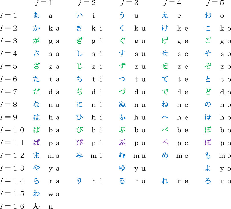
Figure 2. Systematic table of the Japanese syllabary S_ij (i = 1 to 16; j = 1 to 5). The morphologies of letters result from a modification of a very cursive style of writing Chinese characters. The variables i and j, respectively, represent the consonant and vowel that are included in a syllabic.

2.2 Statistical method

The ranking of cumulative frequencies (using variables x and y, respectively) of the 45 syllabics that are contained in the sequence of dialectal variants for snails will be analyzed statistically. To our knowledge, a rank-frequency rule was initially found by Serge Frontier (1934–2011), French marine biologist, for the diagrammatic analysis of ecosystems [23]. In this paper, a similar rule is utilized for the analysis of a nonreciprocal language change. First of all, we note that one of the most outstanding linguistic achievements in recent years can be found in the Linguistic Atlas Project (LAP) for the United States and southern Canada [8–11]. According to the atlas, the frequencies of responses versus their ranks obey necessarily a distinctly long-tailed distribution. Namely, there are a few terms that are very common, a handful terms that are fairly common, and many terms that occur only a couple of times. What is the most surprising is that the rule can be found in every kind of language data that include lexicon, syllables, pronunciation, and grammar. But the specific form of the long-tailed function depends on the data. For statistics in word association surveys, where the size of data exceeds a hundred, one can see a substantially long tail being best fitted to a power law relation. For the analysis of syllabic as well as letter occurrences, however, in which at most tens of categorial data are dealt with, the length of tails is not as long as the one in the so-called Zipf’s law for the word statistics, where usually words of tens of thousands in number are dealt with [13]. Hence, in this paper, as a specific form of the moderately long-tailed profile we concentrate on the logarithmic function, the validity of which has been established for the general competitive systems with the moderate size of data [24, 25] as well as for the alphabetical statistics for the analysis of English texts [26, 27],

$y=a–b\log x,(1)$

where log abbreviates the common logarithm (log₁₀); y corresponds to the cumulative frequency of each individual N syllabics that are contained in the words appearing from the start (n = 1) to the present site (n = k; k = 2, … , 134); x represents the rank variable in descending order. Namely, x = 1 for y = y₍₁₎, x = 2 for y = y₍₂₎, ・・・, and x = N for y = y_(N), where y_(i) indicates the ordered statistics of y_i (y_i with suffix i indicates the cumulative frequency of the i-th syllabic) as y₍₁₎ > y₍₂₎ > ・・・> y_(N). The parameters a and b are positive constants to be determined with the least square fit. The validity of regression can be quantified with the degree of fit, |r|, i.e., with the Pearson’s coefficient (0 < |r| < 1; note that in our regression analysis the value of r is always negative), and with the Durbin-Watson ratio, d (0 < d < 2 for positive serial correlations, whereas 2 < d < 4 for negative counterparts; d = 2 for null correlation) [28–34]. The formulae necessary for calculating the degree of fit, |r|, and the Durbin-Watson ratio, d, respectively, are

$r=\frac{s_{uv}}{s_u{s}_v},(\mathrm{2a})$

$s_{uv}=\frac{1}{N}{\displaystyle \sum _{i=1}^N}{u}_i{v}_i-m_u{m}_v,(\mathrm{2b})$

$s_u^2=\frac{1}{N}{\displaystyle \sum _{i=1}^N}{u}_i^2-m_u^2,(\mathrm{2c})$

$s_v^2=\frac{1}{N}{\displaystyle \sum _{i=1}^N}{v}_i^2-m_v^2,(\mathrm{2d})$

$m_u=\frac{1}{N}{\displaystyle \sum _{i=1}^N}{u}_i,(2e)$

$m_v=\frac{1}{N}{\displaystyle \sum _{i=1}^N}{v}_i,(\mathrm{2f})$

$d=\frac{1}{N-1}{\displaystyle \sum _{i=1}^{N-1}}{\left(p_{i+1}-p_i\right)}^2,(\mathrm{3a})$

$p_i=\frac{e_i}{s},(\mathrm{3b})$

$e_i=v_i-v_i^{\prime },(\mathrm{3c})$

$s^2=\frac{1}{N-1}{\displaystyle \sum _{i=1}^{N-1}}{e}_i^2,(\mathrm{3d})$

where (u, v) = (log x, y), and in Equation 3c v’ indicates the point on the regression line (Equation 1). Note that, because of the reason mentioned in the preceding subsection, N = 45. In contrast to non-ranking as well as rank-rank data (such as, e.g., Spearman’s or Kendall’s approach), for the rank-size or rank-frequency analysis, in most cases, positive correlations are seen between the neighboring data [24, 25]. Therefore, not merely as |r| → 1, but also as d → 2, the long-tailed nature of Equation 1 can be regarded as authentic. It should be stressed again that analysis with sole use of the Pearson’s regression, |r|, seems to be unreliable, i.e., for accomplishing our purpose the simultaneous use of the Pearson’s and Durbin-Watson statistic is necessary [24, 25, 28–34]. The use of the latter enables one to discriminate the authentic fitting from the apparent one. For more detailed explanation of the meaning of the ratio d as well as of how it is related to actual data, see the illustrations of Figures 3C, 4C.

Figure 3

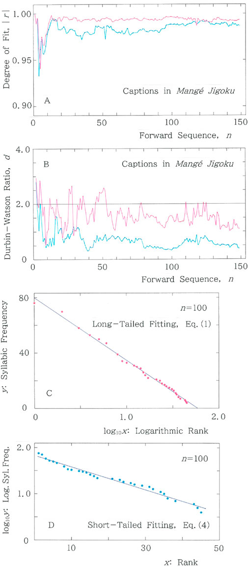
Figure 3. Example results for a series of captions in Mangé Jigoku, where fitting to the long-tailed function (Equation 1) is plotted with the red ink, while the one to the short-tailed function (Equation 4) is plotted with the blue ink. (A) Sequential variations of the degree of fit, |r|, to the long and short tailed distributions for the cumulative syllabic frequency versus rank. Mean values of |r| are (0.992, 0.984), where the left (right) numeral in the parentheses indicates the value of the long (short) tail. (B) Sequential variations of the Durbin-Watson ratio, d. Mean values of d are (1.58, 0.678) (C) Cross-sectional plot of Equation 1 at n = 100, where (|r|, d) = (0.997, 1.569) and (a, b) = (79.77, 45.09). (D) Cross-sectional view of Equation 4 at n = 100, where (|r|, d) = (0.988, 0.328) and (a, b) = (1.83, 2.47 × 10⁻²).

Figure 4

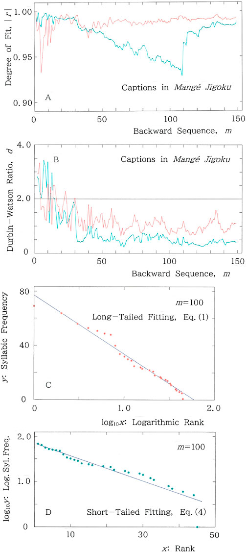
Figure 4. Example results for a series of captions in Mangé Jigoku, where fitting to the long (short) tailed function is plotted with the red (blue) ink. (A) Backward sequential variations of the degree of fit, |r|, to the long and short tailed distributions for the cumulative syllabic frequency versus rank. (B) Backward sequential variations of the Durbin-Watson ratio, d. (C) Cross-sectional plot of Equation 1 at m = 100, where (|r|, d) = (0.988, 0.677) and (a, b) = (77.04, 43.53). (D) Cross-sectional view of Equation 4 at m = 100, where (|r|, d) = (0.945, 0.456) and (a, b) = (1.85, 2.78 × 10⁻²).

To monitor the validity of the long-tailed hypothesis of Equation 1, at the same time we consider a function with a short-tailed decay bearing dual relation with Equation 1

$\log y=a–bx.(4)$

Again, the parameters a and b are positive constants to be determined with the least square fit, and in using the formulae of Equation 2a–f and Equation 3a–d, (u, v) = (x, log y)

3 Examples for testing methodology

To examine the validity of our method, in this section we first consider a few examples: sequence of captions in a novel, and of fictitious characters in an animation, followed by passages being sampled from a novel.

3.1 Sequence of captions

Figure 3 shows the results for a series of captions (titles of chapters) in Mangé Jigoku [35], “Kaleidoscopic Hell,” a tale of the bizarre written in 1929 by Eiji Yoshikawa (1892–1962), who was known, along with Akiko Yosano (1878–1942), for a composer of novel words, but was far from an idioglossia. The figure includes (A) sequential variations of the degree of fit, |r|, to the long and short tailed distributions for the cumulative syllabic frequency versus rank and (B) the ones of the Durbin-Watson ratio, d. In both (A) and (B), fitting to the long (short) tailed function, Equation 1 (Equation 4), is plotted with the red (blue) ink. For instance, at n = 100, the coordinates of data are (x, y) = (1, 76), (2, 70), (3, 58), (4, 53), (5, 50), … …, (43, 6), (44, 5), (45, 4); for the regression of Equation 1 with a long tail, they yield (|r|, d) = (0.997, 1.569) on the red line, while for the regression of Equation 4 with a short tail, (|r|, d) = (0.988, 0.328) on the blue line. The cross-sectional plot of Equation 1 at n = 100 is given in Figure 3C, where one can see that red points are almost randomly dispersed in the vicinity of the regression line, though the randomness is not perfect because 2 – d = 0.431, and consequently the value of |d – 2| does not exactly vanish. Note that perfect randomness is achieved solely for d = 2.000. The cross-sectional plot of Equation 4 at n = 100 is given in Figure 3D, where one can see that, as is evident from 2 – d = 1.672, blue points are far from randomly dispersed across the regression line.

Not to mention music [12–14], time reversal asymmetries (TRAs) can be seen ubiquitously for sequences of numerical data not obeying Gaussian characteristics [15]. For the sequences of categorial data as well it sounds reasonable to expect such asymmetries. The backward counterpart of Figure 3 is given in Figure 4. Namely, for a series of captions in Mangé Jigoku, we show (A) backward sequential variations of the degree of fit, |r|, to the long and short tailed distributions for the cumulative syllabic frequency versus rank, and (B) the ones of the Durbin-Watson ratio, d. In both (A) and (B), fitting to the long (short) tailed function, Equation 1 (Equation 4), is plotted with the red (blue) ink. For instance, at m = 100, the coordinates of data are (x, y) = (1, 69), (2, 64), (3, 56), (4, 53), (5, 51), … …, (43, 6), (44, 5), (45, 1); for the regression of Equation 1 with a long tail, they yield (|r|, d) = (0.988, 0.677) on the red line, while for the regression of Equation 4 with a short tail, (|r|, d) = (0.945, 0.456) on the blue line. The cross-sectional plot of Equation 1 at m = 100 is given in Figure 4C, where one can see that, in sharp contrast to the ones in Figure 3C, the red points oscillate sinusoidally across the regression line. Namely, as is expected from |d – 2| = 1.323, the dispersion appears far from random. In comparison between Figure 3C (with |d – 2| = 0.431) and Figure 4C (with |d – 2| = 1.323), one can realize the significance of the Durbin-Watson analysis. The cross-sectional plot of Equation 4 at m = 100 is given in Figure 4D, where one can see that, as is evident from |d – 2| = 1.544, blue points are far from randomly dispersed across the regression line.

Incidentally, it can be seen that for the blue line in Figure 4A an abrupt jump occurs at m = 110, where the magnitude of |r| for the short-tailed fitting (Equation 4) increases from 0.928 to 0.965. The discontinuity arises from the abrupt change (specifically, from 1 to 2) in the cumulative frequency of the last-place syllabic /S₉₄/ being defined in Figure 2. It should be stressed here that in general the short-tailed fitting is much more sensitive to the magnitude of an exceptional datum than the long-tailed counterpart.

To reveal the TRAs more distinctly, in Figure 5A scattergram is shown for n = m of the red lines (i.e., fitted to Equation 1) in Figures 3, 4. Here the degree of fit and the Durbin-Watson ratio, respectively, are plotted in Figures 5A, B. In the former there are two regions sectioned by y = x, while in the latter there are four sections (I–IV) that are divided by the twin lines crossed perpendicularly on (x, y) = (2, 2):

$\left|y–2\right|<\left|x–2\right|\text{for\hspace{0.17em}Section\hspace{0.17em}}\mathrm{I}\text{\hspace{0.17em}and\hspace{0.17em}III},(\mathrm{5a})$

$\left|y–2\right|>\left|x–2\right|\text{for\hspace{0.17em}Section\hspace{0.17em}II\hspace{0.17em}and\hspace{0.17em}IV}.(\mathrm{5b})$

Figure 5

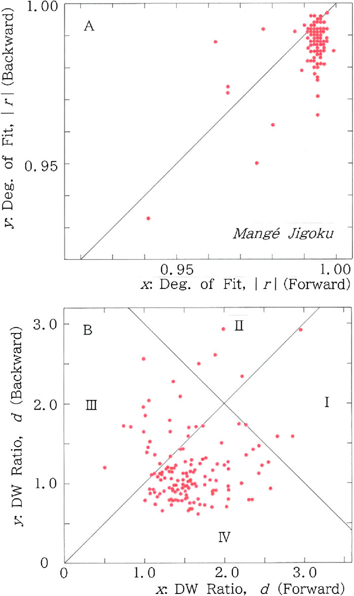
Figure 5. Scattergrams for n = m of the red lines (i.e., fitted to the long-tailed function, Equation 1) in Figures 3, 4. (A) Degree of fit. Mean: (x, y) = (0.992, 0.988); CV: (x, y) = (0.007, 0.008). (B) Durbin-Watson ratio. Mean: (x, y) = (1.58, 1.19); CV: (x, y) = (0.268, 0.397).

Note that neither x nor y in the context of Equation 5a, b has anything to do with the same letters used in the preceding section. Examining the concentration of scatter points in the two (Figure 5A) and four (Figure 5B) regions, respectively, allows one to conclude that, if there exist more points being plotted in the lower region than those in the upper region (Figure 5A), and at the same time, there are more points in Section II or IV than those in Section I or III (Figure 5B), the sequence under consideration exhibits the TRA. Specifically in Figure 5A we find 127 points for the lower region (y < x), in contrast to 20 points for the upper one (y > x). In Figure 5B we find 122 points in Section II or IV, while 25 points in Section I or III.

3.2 Sequence of fictitious characters

Subsequently example results are shown in Figure 6 for a parade of fictitious monsters in Pokémon [36]. The figure is composed with (A) sequential variations of the degree of fit, |r|, to the long and short tailed distributions for the cumulative syllabic frequency versus rank, and (B) the ones of the Durbin-Watson ratio, d. In both (A) and (B), fitting to the long (short) tailed function, Equation 1 (Equation 4), is plotted with the red (blue) ink. To examine the TRA in the sequence, example results are given in Figure 7 for the reverse of fictitious monsters in Pokémon. Here we show (A) backward sequential variations of the degree of fit, |r|, to the long and short tailed distributions for the cumulative syllabic frequency versus rank, and (B) the ones of the Durbin-Watson ratio, d. In (A) and (B), fitting to the long (short) tailed function, Equation 1 (Equation 4), is plotted with the red (blue) ink. Comparisons between Figures 6A, 7A and between Figures 6B, 7B suggest the existence of the TRA. Namely, it seems that composers of the fictitious monsters created them according to a hidden rule that starts from a relatively archaic naming toward a somewhat exotic one.

Figure 6

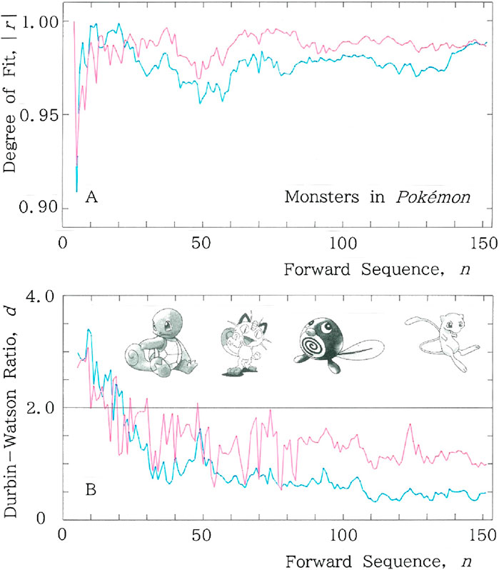
Figure 6. Example results for a parade of fictitious monsters in Pokémon. In both A and B, fitting to the long-tailed function (Equation 1) is plotted with the red ink, while the one to the short-tailed function (Equation 4) is plotted with the blue ink. (A) Sequential variations of the degree of fit, |r|, to the long and short tailed distributions for the cumulative syllabic frequency versus rank. Mean values of |r| are (0.986, 0.977), where the left (right) numeral in the parentheses indicates the value of the long (short) tail. (B) Sequential variations of the Durbin-Watson ratio, d. Mean values of d are (1.41, 0.931).

Figure 7

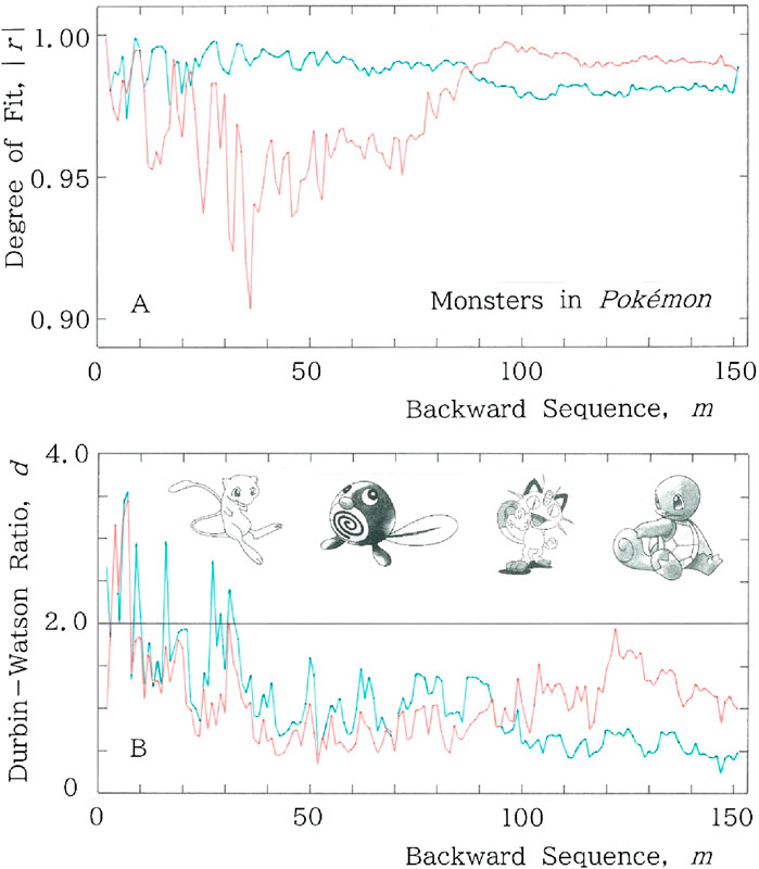
Figure 7. Example results for a parade of fictitious monsters in Pokémon. In A and B, fitting to the long (short) tailed function is plotted with the red (blue) ink. (A) Backward sequential variations of the degree of fit, |r|, to the long and short tailed distributions for the cumulative syllabic frequency versus rank. (B) Backward sequential variations of the Durbin-Watson ratio, d.

Incidentally, careful comparison between Figures 6, 7 suggests that for m < 100 the short-tailed fitting of the backward sequence becomes better than the forward counterpart. Indeed, calculation of the mean values shows |r|: 0.977, d: 0.931 for the forward sequence, while |r|: 0.986, d: 1.02 for the backward sequence. This behavior, which appears somewhat curious, can be explained as follows: Consider for instance n = m = 61, respectively, in Figures 6, 7. Inspection of the rank-frequency relation for the backward sequence has shown a tail shorter than the forward one. Specifically, for the former (Figure 7) the tail extends down to Rank 38, while for the latter (Figure 6) to Rank 41. To quantitatively explain the behavior, comparison between entropy has been carried out, which yields (H (nat), h) = (3.34, 0.876) for the backward sequence; (H (nat), h) = (3.45, 0.906) for the forward sequence, where H (nat) and h, respectively, indicate the information entropy being measured in the natural unit, nat for short, and the relative entropy (0 < h < 1). It is found that the lower entropy for the former (Figure 7) is consistent with the shorter tail in the rank-frequency distribution.

To analyze the asymmetry in more details and to make an appeal to our eyes, the scattergrams are given in Figure 8. While in Figure 8A one finds 75 points for the lower region (y < x) in contrast to 71 points for the upper one (y > x), in Figure 8B we find 95 points in Section II or IV, while 51 points in Section I or III.

Figure 8

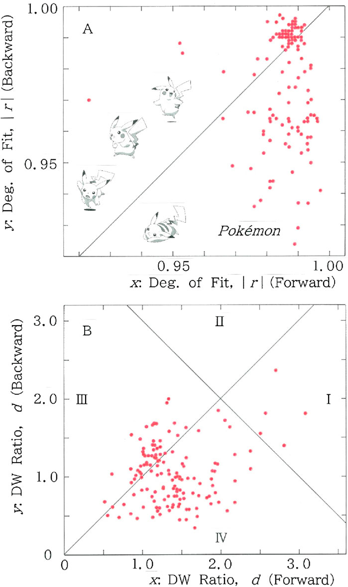
Figure 8. Scattergrams for n = m of the red lines (i.e., fitted to the long-tailed function, Equation 1) in Figures 6, 7. (A) Degree of fit. Mean: (x, y) = (0.986, 0.975); CV: (x, y) = (0.009, 0.020). (B) Durbin-Watson ratio. Mean: (x, y) = (1.41, 1.07); CV: (x, y) = (0.338, 0.431).

3.3 Why TRA occurs

Through the two examples above, it has been shown that the TRA arises from the sequence of captions in a novel (Figures 3–5) and from the sequence of names of fictitious characters (Figures 6–8). To our knowledge, the asymmetry will be ubiquitous in the general Markovian sequences of time-series names. Here, names include those for persons, animals, plants, places, chapters, and so on. To explain qualitatively the reason why the asymmetry occurs and at the same time how to reveal it from our approach to syllabic data, an imaginary story in what follows may be useful: Suppose a boy who has been assigned to the post for creating nicknames of forty classmates (assuming N_i with i = 1, 2, … , 40). The teacher in charge of the class is assumed to put no restrictions but duplication. Namely, no one is allowed to have the nickname identical to the others. At first, the pupil is supposed to be able to create nicknames very easily because there are rich choices available. But as the naming proceeds, he will suffer from a frustration because he is about to exhaust his resources for vocabulary. It should be noted here that he ought to be bound not only by the explicit rule imposed by the teacher (i.e., inhibition of the duplication) but also by several implicit rules such as avoidance of words that are contrary to morals as well as of those implying sneer, taunt, scoff, scorn, or derision. Furthermore, he ought to be bound unconsciously by a sound pattern inherent in his native language. After a while, the boy will find a compromise by generating names being slightly modified from the preceding ones, which may necessarily include a certain reduplication, i.e., the repetitive use of the same word root. The tactics, however, seem to be responsible for enhancing redundancy in the latter part of the sequence. Next suppose that the resultant sequence of the forty nicknames is analyzed with our method mentioned in Section 2.2. For the forward analysis (i.e., usual reading: N₁→ N₂ → … … → N₃₉→N₄₀) the cumulative frequencies of syllabics versus their ranks are expected to obey the long-tailed distribution of Equation 1. Namely, there will be a few syllabics that are very common, a handful syllabics that are fairly common, and many syllabics that occur only a couple of times [9–11]. In contrast to the usual reading, for the backward counterpart (unusual reading: N₄₀→ N₃₉ → … … →N₂ →N₁), at the beginning part in particular, the cumulative frequencies of syllabics versus their ranks are supposed to exhibit a distribution far from long tailed because the contents of syllabary will be occupied by several syllabics that are very common, followed by several syllabics that are uncommon.

The above statement suggests that time-dependent juxtapositions of words more or less preserve long range correlations in which the choice of syllabics in the latter part of the sequence depends on the choice in the former [37, 38]. To examine the hypothesis in more detail, here we consider a text, i.e., passages in a novel written with Japanese. Example results are shown in Figure 9 for passages being sampled from Shiiku [39], “The Catch,” a short novel written by Kenzaburo Oe (1935–2023), a Japanese Nobel laureate for literature in 1994. Note that the passages are composed of 79 words. Figure 9A shows the sequential variations of the degree of fit, |r|, to the long and short tailed distributions for the cumulative syllabic frequency versus rank. It can be seen that the result shares main features with those seen in Figures 3A, 6A. Subsequently, sequential variations of the Durbin-Watson ratio, d, are given in Figure 9B, showing the feature in common with those seen in Figures 3B, 6B. The backward counterpart of (A) and (B), respectively, are shown in Figures 9C, D. One can see that these are consistent with those given in Figures 4A, B. To conclude, unusual reading of texts gives rise to unusual results as if a tune were played reversely (For the discussion of music, see Figure 15).

Figure 9

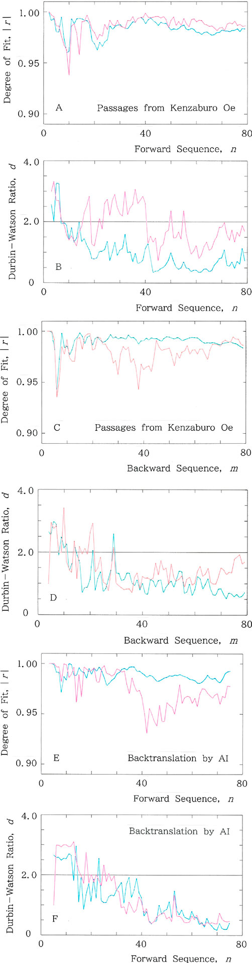
Figure 9. Example results for passages being sampled from Shiiku, a short novel written by Kenzaburo Oe. Note that in A to E, fitting to the long-tailed function (Equation 1) is plotted with the red ink, while the one to the short-tailed function (Equation 4) is plotted with the blue ink. (A) Sequential variations of the degree of fit, |r|, to the long and short tailed distributions for the cumulative syllabic frequency versus rank, where Mean: |r| = 0.987 for Equation 1, while Mean: |r| = 0.983 for Equation 4. (B) Sequential variations of the Durbin-Watson ratio, d, where Mean: d = 1.854 for Equation 1, while Mean: d = 0.977 for Equation 4. (C) Backward counterpart of A. Here Mean: |r| = 0.980 for Equation 1, while Mean: |r| = 0.990 for Equation 4. (D) Backward counterpart of B. Here Mean: d = 1.473 for Equation 1, while Mean: d = 1.190 for Equation 4. (E) Computed results of |r| versus n for the text that has been back-translated by AI from an English version of the original text in Japanese, where Mean: |r| = 0.974 for Equation 1, while Mean: |r| = 0.989 for Equation 4. (F) Durbin-Watson counterpart of E, where Mean: d = 1.233 for Equation 1, while Mean: d = 1.170 for Equation 4.

Finally, in an effort to confirm the long-range hypothesis, a backtranslation experiment [40] has been carried out utilizing artificial intelligence (AI) in a free machine-translation device offered by Google. Example results are given in Figures 9E, F. Figure 9E shows computed results of |r| versus n for the text that has been back-translated by AI from an English version [41] of the original text in Japanese [39]. Subsequently Figure 9F shows the Durbin-Watson counterpart of (E). Note that in A to F, fitting to the long-tailed function (Equation 1) is plotted with the red ink, while the one to the short-tailed function (Equation 4) is plotted with the blue ink. As might have been expected, both results (Figures 9E, F) indicate that AI cannot reproduce the long-tailed distribution of Equation 1, which can be explained by noticing the fact that AI uses in principle a word-for-word translation or at best a translation with short-range correlations. The above results seem to aptly demonstrate that the long-range correlations in texts arise from the ability only to be found in the human intelligence.

4 Results of dialectal variants for snails

4.1 Statistical analysis

Now that through the results shown in Figures 3–9 the validity of our methodology has been established, we shall apply it to the syllabic data of dialectal variants for snails, in an effort to test the Yanagita’s theory of the concentric distribution of the dialectal words [1]. In Figure 10, results of dialectal variants for snails are shown for (A) periphery-to-center (Group A to E) sequence of the degree of fit, |r|, to the long and short tailed distributions for the cumulative frequency of 45 syllabics versus the rank, and (B) the one of the Durbin-Watson ratio d. In both A and B, fitting to the long (short) tailed function, Equation 1 (Equation 4), is plotted with the red (blue) ink. It can be seen that in contrast to the prior results (Figures 3A, 6A), in Figure 10A, red and blue lines are entangled each other, but in the almost entire region of Figure 10B the d value of the red line (Equation 1) is larger than the one of the blue one (Equation 4). At n = 100 the original and rank-ordered histograms, respectively, are shown in Figures 10C, D.

Figure 10

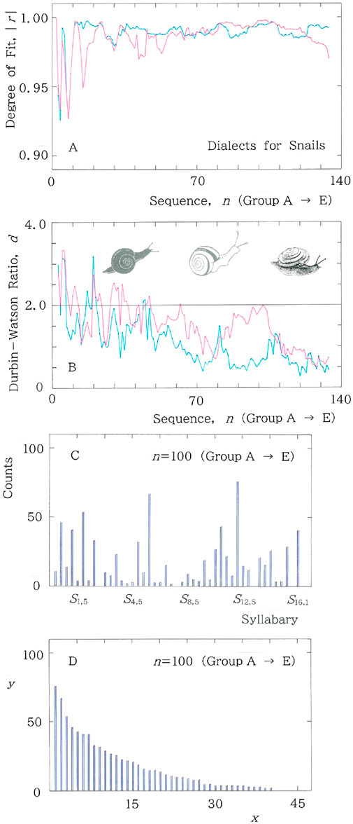
Figure 10. Results of dialectal variants for snails. In both A and B, fitting to the long-tailed function (Equation 1) is plotted with the red ink, while the one to the short-tailed function (Equation 4) is plotted with the blue ink. (A) Periphery-to-center sequence of the degree of fit, |r|, to the long and short tailed distributions for the cumulative syllabic frequency versus rank. (B) Periphery-to-center sequence of the Durbin-Watson ratio, d. It can be seen that in contrast to the prior results (Figures 3A, 6A), in Figure 10A, red and blue lines are entangled each other, but in the almost entire region of Figure 10B the d value of the red line (Equation 1) is larger than the one of the blue one (Equation 4). (C) Histogram at n = 100 in the periphery-to-center sequence of the dialectal variants for snails. (D) Rank-ordered arrangement for which regressions of Equation 1 and Equation 4 will be made. Specifically, (|r|, d) = (0.998, 1.826) for Equation 1, while (|r|, d) = (0.995, 0.567) for Equation 4. Although the |r| values are extremely high in both regressions and at the same time are comparable each other, comparison between the d values indicates that the envelope of Figure 10D fits much better with the long-tailed function (Equation 1) than with the short-tailed counterpart (Equation 4).

Subsequently, results of the dialectal variants for snails are given in Figure 11A for center-to-periphery (Group E to A) sequence of the degree of fit, |r|, to the long and short tailed distributions for the cumulative frequency versus rank, and in Figure 11B for the sequence of the Durbin-Watson ratio, d. In both A and B, again, fitting to the long (short) tailed function is plotted with the red (blue) ink. At m = 100 the original and rank-ordered histograms, respectively, are shown in Figures 11C, D, which will be compared with Figures 10C, D.

Figure 11

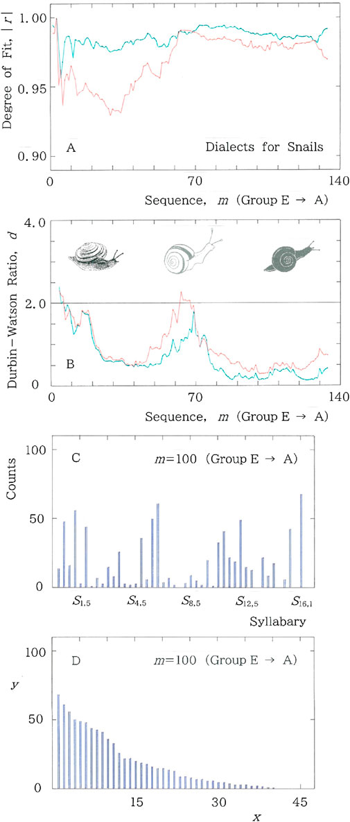
Figure 11. Results of dialectal variants for snails. In both A and B fitting to the long (short) tailed function is plotted with the red (blue) ink. (A) Center-to-periphery sequence of the degree of fit, |r|, to the long and short tailed distributions for the cumulative syllabic frequency versus rank. (B) Center-to-periphery sequence of the Durbin-Watson ratio, d. (C) Histogram at m = 100 in the center-to-periphery sequence of the dialectal variants for snails. (D) Rank-ordered arrangement for which regressions of Equation 1 and Equation 4 will be made. Specifically, (|r|, d) = (0.978, 0.319) for Equation 1, while (|r|, d) = (0.988, 0.159) for Equation 4. There is a hump around x = 10. It should be noted that both the |r| and d values are much smaller than those given in the caption of Figures 10C, D.

For m < 60 in Figure 11A the behavior of |r| bears a resemblance to the afore-mentioned one in Figure 7A. Choose for instance m = 32, where |r| = 0.933 for the long-tailed fitting, Equation 1, while |r| = 0.976 for the short-tailed fitting, Equation 4. Calculation of the information entropy and the relative entropy gives, respectively, H (nat) = 2.75 and h = 0.723, both of which are lower than those at n = 32 in Figure 10A: H (nat) = 2.88 and h = 0.758. Again, the lower entropy seems to be responsible for reducing the long-tailed fitting.

In Figures 12A, B, scattergrams are plotted for the results of the red lines in Figures 10, 11. Specifically in Figure 12A we find 116 points for the lower region (y < x), in contrast to only 15 points for the upper one (y > x). In Figure 12B we find 99 points in Section II or IV, while 32 points in Section I or III.

Figure 12

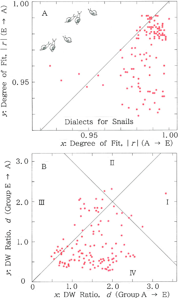
Figure 12. Scattergrams for n = m of the red lines (i.e., fitted to the long-tailed function, Equation 1) in Figures 10, 11. (A) Degree of fit. Mean: (x, y) = (0.986, 0.969); CV: (x, y) = (0.012, 0.018). (B) Durbin-Watson ratio. Mean: (x, y) = (1.52, 0.937); CV: (x, y) = (0.380, 0.632).

Qualitatively, the remarkable TRA in the dialectal wave propagation can be explained in part with the frequent use of a specific radical such as /S_7,4S_16,1/ in Group E, which makes the sequence in this group considerably pleonastic. In contrast, one can find no remarkable pleonasm in Group A to C. The reason why such a bias tends to occur in Markovian name sequences, on which avoidance of the perfect duplication is strictly imposed, has been detailed in Section 3.3. In summary, composers of the dialectal words seem to relieve their frustration through finding a compromise in the naming process. The mandatory requirement for avoiding duplication in the entire word is responsible for the increasing use of a specific sound component in a word.

4.2 Statistical testing

To establish the authenticity of the TRA for the propagation of the dialectal variants for snails, we will make a binomial test (with α denoting significant level) for the hypothesis that the time series is reversible [42]. With p being the probability of finding a point in the target (i.e., the lower region of Figure 12A and simultaneously Section II or IV in Figure 12B), we start from

$H:p={\left(1/2\right)}^2=1/4,K:p>1/4,(6)$

where H and K, respectively, are the null and the alternative hypothesis. Because of 97 points being seen in the target, according to the Fisher’s methodology the cumulative probability of the frequency can be calculated as follows:

$P\left(97\le X\le 131\right)={\sum }_x{}_{131}{C}_x{\left(1/4\right)}^x{\left(3/4\right)}^{131–x}\fallingdotseq 2.35\times {10}^{-30},(7)$

where summation should be made from x = 97 to 131. Therefore, for α = 10^–29 the null hypothesis H is rejected. Namely, the series of the dialects for snails is not reversible.

It should be noted here that the dialectal data for snails had been collected by a single scholar, i.e., Yanagita himself [1], without recording devices being available, which might admit of arbitrariness due, for instance, to transcription errors, in addition to a cognitive bias of the listener. To respond to this potential concern, we consider modified data in which the endings of all the dialectal words for snails are truncated. Analysis has shown that, instead of the 97 points for the original data, for the perturbed ones there are 93 points being seen in the target. The cumulative probability of the frequency is replaced by

$P\left(93\le X\le 131\right)={\sum }_x{{}_{131}C}_x{\left(1/4\right)}^x{\left(3/4\right)}^{131–x}\fallingdotseq 2.97\times {10}^{-28},(8)$

where summation is made from x = 93 to 131. Therefore, for α = 10^–27 the null hypothesis H is rejected. Namely, in the same way as the unperturbed data the series of the modified dialects for snails is not reversible.

5 Discussion

5.1 Applying most parsimonious principle

To make our approach as multidisciplinary as possible, we shall attempt to make full use of recent achievements in phylogeny [16–18], in which we take notice of the two axioms: 1) The inherited character with higher frequency is more archaic than the one with low frequency; and 2) The phylogenic trees can be reconstructed through taking advantage of the so-called “most parsimonious principle,” where one regards the most inert tree in numbers of characters’ variations as being most plausible.

In Figure 13A the top 15 syllabics are listed in the ranking of 134 dialectal variants for snails, where one can find that, except for the syllabic nasal (S_16,1), the most frequent syllabic is S_12,4 in the table of Figure 2. Subsequently in Figure 13B we extract this syllabic from Figure 13A, in order to illustrate rich connotations inherent in the key syllabic. At the same time, Chinese characters being transliterated reveal seven meanings from the syllabic, all of which evidently suggest significance in the context of depth psychology.

Figure 13

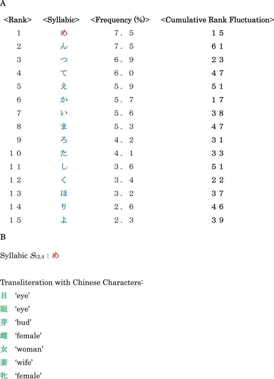
Figure 13. (A) The top 15 syllabics in the ranking of 134 dialectal variants for snails. (B) The most frequent syllabic and its connotations being transliterated with Chinese characters.

In Figure 14 we show sequential plots of (A) the rank variation in the frequency of S_12,4 and (B) the cumulative rank fluctuation (CRF) of the syllabic, which is defined as

$CRF={\sum }_i\left|R_{i+1}–R_i\right|,(9)$

where i = 1 to 133, and R_i denotes the rank of cumulative frequency for the syllabic in the sequence. In the plots the red and green lines indicate, respectively, the periphery-to-center (Group A to E in Figure 1) and the center-to-periphery (Group E to A in Figure 1). Comparison between the two lines in Figure 14B indicates that the entire CRF of the latter (green) amounts to 30, which is twice as large as the former (red). Along with the conceptional borrowing from the most parsimonious principle in phylogeny [16] as well as with the results shown in Figures 10–12, it sounds reasonable to conclude that there is no room to doubt the validity of the Yanagita’s theory that was given in 1927 [1], saying that more archaic dialectal variants tend to live longer in areas extremely far from a stronghold of culture being a point source of a dialectal tsunami.

Figure 14

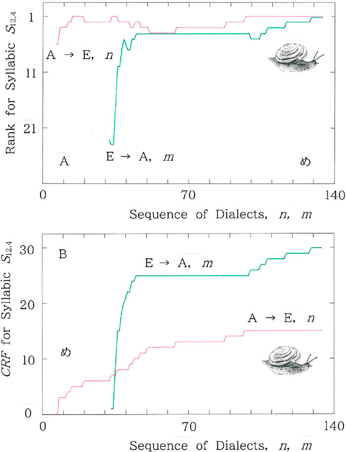
Figure 14. Sequential plots of (A) the rank variation in the frequency of S_12,4 and (B) the cumulative rank fluctuation of the syllabic. The red and green lines indicate, respectively, the periphery-to-center and center-to-periphery.

5.2 Putting artificial disturbance

To make the above conclusion firmer, we consider six imaginary cases in which a dialectal group is permuted according to a prescribed rule. Specifically, the terminal group, Group A or E in Figure 1, is inserted between two subsequent groups. With these permutations, six cases are generated: Case 1. B→A→C→D→E, Case 2. B→C→A→D→E, Case 3. B→C→D→A→E, Case 4. A→B→C→E→D, Case 5. A→B→E→C→D, and Case 6. A→E→B→C→D. In Table 1, along with the original sequence (A→B→C→D→E), comparison is given between results for the original sequence and those obtained for the six cases of the artificially disturbed sequences. Here CV denotes the coefficient of variation (standard deviation divided by mean). It should be emphasized that the value of CRF tends to increase as the perturbation gets larger, and that the values easily exceed 20, in particular, for the last three cases. Besides, in striking contrast to the increase in CRF, the mean values of both |r| and d decrease in comparison with those of the original sequence (0.986 for |r|; 1.52 for d).

Table 1

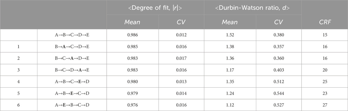
Table 1. Comparison of results for the original sequence and those obtained for six cases of artificially disturbed sequences. CV = coefficient of variation (standard deviation divided by mean); CRF = cumulative rank fluctuation.

6 Notes added for proving methodological potentiality

6.1 Application to popularity ranking of given names

It was found previously that the popularity ranking of given names for a large sample of Japanese boys exhibits a noticeable TRA both in the degree of fitting |r| and in the Durbin-Watson ratio d [43]. Calculation of the mean values has shown, respectively, (0.992, 0.988) and (1.42, 0.61), where the left (right) numeral in the parentheses indicates the forward (backward) reading of the entire name sequence. This result can be explained by a property being inherent in the ranking sequence that starts from a relatively conventional naming being seen in the higher ranking toward a somewhat exotic one in the lower one.

6.2 Application to stochastic music

One can find that one of the advantages of our method lies in its applicability to both numerical and categorial data. To show the applicability to the former we consider three types of stochastic music: white, 1/f (pink or tan), and brown (Brownian) one [12–14], with which the validity of our statistical approach will be tested. The results of the scattergrams are plotted in Figures 15A–C, respectively, for the sequence of pitch in the white, 1/f, and brown music. Here pitch data necessary for calculation have been taken from Gardner [14]. Comparison between Figures 15A–C yields several interesting results: (1) In usual playing, the mean value of the fit for the long-tailed function, |r|, becomes peaked for the 1/f music, i.e., 0.980 (for brown) < 0.981 (for white) < 0.989 (for 1/f). (2) In the reverse playing, the value decreases monotonically in order from white, 1/f, and brown, i.e., 0.984 (for white) > 0.980 (for 1/f) > 0.968 (for brown), and (3) In contrast, the modulus of difference between the usual and reverse playing increases monotonically in the same order, i.e., 0.003 (for white) < 0.009 (for 1/f) < 0.012 (for brown). It should be emphasized that these observations are consistent with those obtained through the conventional analysis of the power spectra of the autocorrelations [12–14].

Figure 15

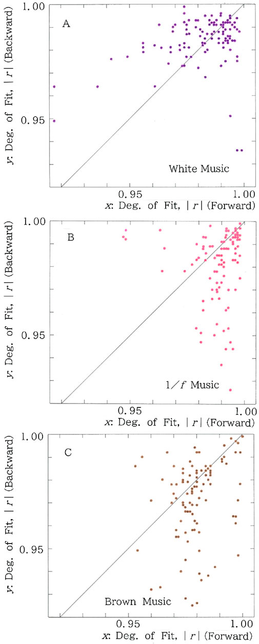
Figure 15. (A) Scattergram for the time series of pitch in the white music. Degree of fit. Mean: (x, y) = (0.981, 0.984); CV: (x, y) = (0.019, 0.012). There are 47 points in the lower region (y < x), in contrast to 74 points in the upper one (y > x). (B) Scattergram for the time series of pitch in the 1/f music. Degree of fit. Mean: (x, y) = (0.989, 0.980); CV: (x, y) = (0.010, 0.016). There are 79 points in the lower region (y < x), in contrast to 28 points in the upper one (y > x). (C) Scattergram for the time series of pitch in the brown music. Degree of fit. Mean: (x, y) = (0.980, 0.968); CV: (x, y) = (0.010, 0.025). There are 76 points in the lower region (y < x), in contrast to 36 points in the upper one (y > x).

7 Conclusion

In an effort to aim at settling a long-term controversy in dialectology, we have established quantitatively the validity of the Yanagita’s theory of the concentric distribution of dialectal variants for snails. Although the theory was presented in 1927, since then, for more than 95 years its verification has remained pending. Our statistical method owes much the recent achievement in the Linguistic Atlas Project. Specifically, time series analysis has been made with fitting to the long-tailed rank-frequency relations of cumulative syllabics that are included in the entire dialectal sequence of snails. Computed results have shown substantial time reversal asymmetries between the periphery-to-center and center-to-periphery analysis for fitting to the long-tailed distribution in the cumulative syllabic frequency versus the rank. It should be noted that this feature for our categorial data sequence is consistent with those observed for typical numerical data such as brown or pink music as well as heartbeat signals that obey non-Gaussian statistics. Application to the most parsimonious principle that had been developed in the context of phylogenetic data analyses has yielded results being compatible with the above ones, which has reproduced the validity of our conclusion. Finally, perturbation analysis for several artificially disturbed arrangements of the dialectal strata has yielded results that can support our conclusion. Lastly the methodology presented here will be applicable to the epidemic of forenames and other fashion waves that have relevance close to dialects.

Data availability statement

Publicly available datasets were analyzed in this study. This data can be found here: Yanagita, K. (1980) Kagyuko. Tokyo: Iwanami-Shoten.

Author contributions

KH: Writing–original draft, Writing–review and editing.

Funding

The author declares that no financial support was received for the research, authorship, and/or publication of this article.

Conflict of interest

The author declares that the research was conducted in the absence of any commercial or financial relationships that could be construed as a potential conflict of interest.

The author declared that he was an editorial board member of Frontiers, at the time of submission. This had no impact on the peer review process and the final decision.

Publisher’s note

All claims expressed in this article are solely those of the authors and do not necessarily represent those of their affiliated organizations, or those of the publisher, the editors and the reviewers. Any product that may be evaluated in this article, or claim that may be made by its manufacturer, is not guaranteed or endorsed by the publisher.

References

1. Yanagita K. Kagyuko. Tokyo, Japan: Iwanami-Shoten (1980) (originally published in 1927 by the Anthropological Society of Nippon, Tokyo, and subsequently in 1930 by Toko-Shoin, Tokyo).

Google Scholar

2. Ramsey SR. Language change in Japan and the odyssey of a teisetsu. J Jpn Stud (1982) 8:97–131. doi:10.2307/132278

CrossRef Full Text | Google Scholar

3. Lizana L, Mitarai N, Sneppen K, Nakanishi H. Modeling the spatial dynamics of culture spreading in the presence of cultural strongholds. Phys Rev E (2011) 83:066116. doi:10.1103/physreve.83.066116

PubMed Abstract | CrossRef Full Text | Google Scholar

4. Simmel G. Fashion. Am J Sociol (1957) LXII(6):541–58.

CrossRef Full Text | Google Scholar

5. Lieberson S. A matter of taste: how names, fashions, and culture change. New Haven, Connecticut, United States: Yale University Press (2000).

Google Scholar

6. Mateos P. Names, ethnicity and populations: tracing identity in space. Heidelberg, Germany: Springer-Verlag (2014).

Google Scholar

7. Krawczyk MJ, Dydejczyk A, Kułakowski K. The Simmel effect and babies’ names. Physica A (2014) 395:384–91. doi:10.1016/j.physa.2013.10.018

CrossRef Full Text | Google Scholar

8. Kretzschmar WA. Language variation and complex systems. Am Speech (2010) 85:263–86. doi:10.1215/00031283-2010-016

CrossRef Full Text | Google Scholar

9. Kretzschmar WA. Language and complex systems. Cambridge, UK: Cambridge University Press (2015).

Google Scholar

10. Burkette A, Kretzschmar WA. Exploring linguistic science: language use, complexity and interaction. Cambridge, UK: Cambridge University Press (2018).

Google Scholar

11. Kretzschmar WA. Complex systems for corpus linguists. ICAME J (2021) 45:155–77. doi:10.2478/icame-2021-0005

CrossRef Full Text | Google Scholar

12. Voss RV, Clark J. 1/f noise in music: music from 1/f noise. J Acoust Soc Am (1978) 63:258–63.

CrossRef Full Text | Google Scholar

13. Schroeder M. Fractals, chaos, power laws. New York, NY, USA: W. H. Freeman and Company (1991).

Google Scholar

14. Gardner M. Fractal music, hypercards and more … New York. NY, USA: W. H. Freeman and Company (1992).

Google Scholar

15. Hou F, Huang X, Chen Y, Huo C, Liu H, Ning X. Combination of equiprobable symbolization and time reversal asymmetry for heartbeat interval series analysis. Phys Rev E (2013) 87:012908. doi:10.1103/physreve.87.012908

PubMed Abstract | CrossRef Full Text | Google Scholar

16. Sober E. Reconstructing the past: parsimony, evolution, and inference. Cambridge, MA, United States: MIT Press (1989).

Google Scholar

17. Minaka N. Algebraic properties of the most parsimonious reconstructions of the hypothetical ancestors on a given tree. Forma (1993) 8(4):277–96.

Google Scholar

18. Fraix-Burnet D, D’Onofrio M, Marziani P. Phylogenetic analyses of quasars and galaxies. Front Astron Space Sci (2017) 4:20. doi:10.3389/fspas.2017.00020

CrossRef Full Text | Google Scholar

19. Comrie B, editor. The world’s major languages. Oxford, UK: Oxford University Press (1990).

Google Scholar

20. Ruhlen M. A guide to the languages of the world. Stanford, CA, USA: Stanford University Press (1976).

Google Scholar

21. Hayata K. Phonological rules of present-day Japanese in sign-language dictionaries. J Quantitative Linguistics (2017) 24:367–78. doi:10.1080/09296174.2017.1314907

CrossRef Full Text | Google Scholar

22. Hayata K. Frustration in the pattern formation of polysyllabic words. Front Phys (2017) 4:50. doi:10.3389/fphy.2016.00050

CrossRef Full Text | Google Scholar

23. Frontier S. Utilisation des diagrammes rang-fréquence dans l’analyse des écosystèmes. J de Recherche Océanographique (1976) I:35–48.

Google Scholar

24. Hayata K. Statistical properties of extremely squeezed configurations: a feature in common between squared squares and neighboring cities. J Phys Soc Jpn (2003) 72:2114–7. doi:10.1143/jpsj.72.2114

CrossRef Full Text | Google Scholar

25. Hayata K. Birth, annexation, and squeezing of cities in a prefecture: can the ranking of competitive areas of municipalities obey the authentic power law? Front Phys (2022) 9:789571. doi:10.3389/fphy.2021.789571

CrossRef Full Text | Google Scholar

26. Kanter I, Kessler DA. Markov processes: linguistics and Zipf’s law. Phys Rev Lett (1995) 74:4559–62. doi:10.1103/physrevlett.74.4559

PubMed Abstract | CrossRef Full Text | Google Scholar

27. Mantegna RN, Buldyrev SV, Goldberger AL, Havlin S, Peng CK, Simons M, et al. Systematic analysis of coding and noncoding DNA sequences using methods of statistical linguistics. Phys Rev E (1995) 52:2939–50. doi:10.1103/physreve.52.2939

PubMed Abstract | CrossRef Full Text | Google Scholar

28. Durbin J, Watson G. Testing for serial correlation in least squares regression I. Biometrika (1950) 37:409–28. doi:10.1093/biomet/37.3-4.409

PubMed Abstract | CrossRef Full Text | Google Scholar

29. Durbin J, Watson G. Testing for serial correlation in least squares regression II. Biometrika (1951) 38:159–77. doi:10.2307/2332325

PubMed Abstract | CrossRef Full Text | Google Scholar

30. MacKinnon JG. Durbin-Watson statistic. In: The new palgrave dictionary of economics. London, UK: Palgrave Macmillan (2008).

CrossRef Full Text | Google Scholar

31. Chatterjee S, Hadi AS. Regression analysis by example. 5th. Hoboken, NJ, USA: John Wiley and Sons (2012).

Google Scholar

32. Concas G, Congiu F, Muntoni C, Bettinelli M, Speghini A. A hyperfine interaction at Europium sites in oxide glasses. Phys Rev B (1996) 53:6197–202.

PubMed Abstract | CrossRef Full Text | Google Scholar

33. Hill RJ, Flack HD. The use of the Durbin-Watson d statistic in Rietveld analysis. J Appl Cryst (1987) 20:356–61. doi:10.1107/s0021889887086485

CrossRef Full Text | Google Scholar

34. Mesic V, Muratovic H. Identifying predictors of physics item difficulty: a linear regression approach. Phys Rev Spec Top Phys Educ Res (2011) 7:010110. doi:10.1103/physrevstper.7.010110

CrossRef Full Text | Google Scholar

35. Yoshikawa E. Mangé Jigoku. Tokyo, Japan: Kodansha (1968). (originally published in 1929).

Google Scholar

36. Tobin J, editor. Pikachu’s global adventure: the rise and fall of Pokémon. Durham, NC, USA: Duke University Press (2004).

Google Scholar

37. Schenkel A, Zhang J, Zhang Y-C. Long range correlation in human writings. Fractals (1993) 1:47–57. doi:10.1142/s0218348x93000083

CrossRef Full Text | Google Scholar

38. Amit M, Shmerler Y, Eiseenberg E, Abraham M, Shnerb N. Language and codification dependence of long-range correlations in texts. Fractals (1994) 2:7–13.

CrossRef Full Text | Google Scholar

39. Oe K. Shisha no ogori; Shiiku. Tokyo, Japan: Shincho-sha (1959).

Google Scholar

40. Crystal D. The Cambridge encyclopedia of language. Cambridge, UK: Cambridge University Press (1987).

Google Scholar

41. Oe K. The Catch and other war stories. Tokyo, Japan: Kodansha International (1981).

Google Scholar

42. Diks C, van Houwelingen JC, Takens F, DeGoede J. Reversibility as a criterion for discriminating time series. Phys Lett A (1995) 201:221–8. doi:10.1016/0375-9601(95)00239-y

CrossRef Full Text | Google Scholar

43. Hayata K. Selection rules for phonemic patterns in Japanese names concerning families, persons, and places. Inf Sci Bull Gen Res Inst Sapporo Gakuin Univ (2013) 33:1–26.

Google Scholar