Two-dimensional electromagnetic scattering analysis based on the boundary element method

An effective formula for the shape-sensitivity analysis of electromagnetic scattering is presented in this paper. First, based on the boundary element method, a new electromagnetic scattering formula is derived by combining the traditional electromagnetic scattering formula with the non-uniform rational B-spline (NURBS) curve, and the geometric model is represented by NURBS, which ensures the geometric accuracy, avoids the heavy grid division in the optimization process, and realizes the fast calculation of high-fidelity numerical solutions. Second, by deducing the sensitivity variables, the electromagnetic scattering equation of shape optimization is obtained, which can provide reliable data references for shape optimization. Finally, the effectiveness and accuracy of the algorithm are demonstrated by an example, and the sensitivity data of some examples are given.

1 Introduction

At present, the field of radar detection and target stealth design has become a research hotspot, and electromagnetic simulation technology [1] as an indispensable tool in this field is also very important. Commonly used computational electromagnetic methods include finite element method (FEM) [2, 3], boundary element method (BEM) (or method of moment) [4], and finite difference time domain method (FDTD) [5] [6–8]. Among them, the boundary element method is more favored in solving electromagnetic problems because it is only discretized on the surface of the structure and naturally satisfies the radiation condition at infinity. Compared with other domain discretization methods, the boundary element method has higher computational accuracy and smaller degrees of freedom.

Electromagnetic scattering sensitivity analysis has gradually become a hot field with the development of computational electromagnetism. Sensitivity analysis is a statistical method used to observe the behavior or changes in a model by varying its variables within a specific range. It enables the identification and evaluation of relationships between data, systems, or models in order to optimize the model efficiently [9–11]. In the context of electromagnetic scattering, sensitivity analysis aims to explore and analyze how an object or system responds and performs under such conditions. This analysis provides valuable guidance for evaluating object performance and optimizing system design through parameter adjustments [12-14]. Commonly employed methods for electromagnetic scattering sensitivity analysis include derivative-based local approach [15, 16], linear-regression analysis [17-19], and variogram analysis [20, 21] of response surfaces. In this study, we adopted the derivative-based local approach and derived the corresponding shape sensitivity analysis equation through partial differentiation with respect to shape variables. However, the traditional boundary element method employs low-order Lagrange polynomials as basis functions (e.g., Raviart–Thomas [22] or RWG [1] basis functions), which leads to certain limitations: 1) inability to capture intricate details in complex models, resulting in reduced geometric accuracy and 2) utilization of low-order basis functions for approximating physical fields diminishes both the accuracy and sensitivity of the objective function.

The isogeometric analysis (IGA) [23, 24] proposed by Hughes et al. provides a new way to solve the above problems. The key point of IGA is to approximate the physical field by spline function. The use of IGA can avoid repeated mesh division, realize the interaction between Computer Aided Design and Computer Aided Engineering, improve the accuracy of the objective function, and avoid the secondary machining of the model. Isogeometric analysis was first introduced into the finite element method and then quickly generalized to other methods such as the boundary element method. IGA received very wide attention as soon as it was proposed and was quickly applied to elasticity [25–29], fracture mechanics [8, 30–33], acoustic [34–43], fluid mechanics [44–46], flexible composites [9, 47–51], heat conduction [52–55], etc., [56, 57]. However, IGA has not been used in electromagnetism because it needs to meet the divergence and curl coincidence conditions. [58], who proposed B-spline-compatible vector and other geometric finite elements to construct discrete de Rham sequences, made significant achievements in solving this problem [59, 60]. The introduction of compatible B-splines into the boundary element method [61] by Simpson et al. is an important step in the application of the isogeometric boundary element method (IGABEM) in electromagnetics. [62] used the IGABEM to solve the three-dimensional double periodic multilayer structure of electromagnetic scattering problems. [63–65], using the IGABEM combined with the nth-order perturbation method, quantitatively analyzed the uncertainty of the electromagnetic scattering incidence frequency of an antenna array structure. All these have promoted the development of the IGABEM in electromagnetism. In this paper, non-uniform rational B-spline (NURBS) is used as the basis function, and the electromagnetic scattering analysis equation is obtained by combining equal geometry and boundary elements. On this basis, the electromagnetic scattering sensitivity analysis equation for shape sensitivity analysis is derived. To sum up, the innovations of this paper are as follows:

• The formula for electromagnetic scattering analysis is obtained by using the NURBS curve as the basis function

• The IGABEM is used for shape design sensitivity for 2D electromagnetic scattering.

The remainder of this paper is organized as follows: Section 2 gives the IGABEM formula for solving the electromagnetic scattering analysis problem with NURBS as the basis function; Section 3 introduces the shape sensitivity analysis formula with shape design as variables; Section 4 presents two models to verify the accuracy and effectiveness of the IGABEM, and some shape sensitivity data of the models are also given; and Section 5 provides a summary of the paper.

2 Electromagnetic scattering analysis with the Galerkin IGABEM under transverse electric polarization

This section uses the IGABEM. First, the surface current is obtained by solving the surface integral equation, and then the scattering field is obtained by combining the obtained current with the two-dimensional electric field radiation equation. Finally, the two-dimensional radar cross-section is solved by the scattering field and incident field.

2.1 Boundary integral equations

We first assume a bounded field ${\mathrm{\Omega }}_1$ whose connected boundary $\mathrm{\Gamma }$ is in the unbounded field ${\mathrm{\Omega }}_0$ and whose permittivity and permeability are the scalars ${\varepsilon }^0$ and ${\mu }^0$, respectively. An electromagnetic plane wave ${\mathbf{E}}_{\text{inc}}$ with angular frequency $\omega$ is applied to an object with wave number $k=\omega \sqrt{{\epsilon }^0{\mu }^0}$, as shown in Figure 1.

Figure 1

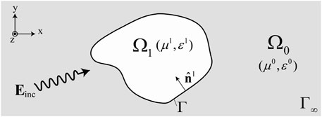
Figure 1. A target structure residing within an infinite domain impinged by an electromagnetic plane wave ${\mathrm{\Omega }}_0$ is the unbounded exterior region to which the free space parameters are assigned $\left({\mu }^0,{\epsilon }^0\right)$; ${\widehat{n}}^1$ denotes the boundary of ${\mathrm{\Omega }}_1$. The normal vector ${\widehat{n}}^1$ points toward the interior of ${\mathrm{\Omega }}_1$ from its interface.

The surface integral equations on $\mathrm{\Omega }$ are as follows:

${\left[\text{i}\omega \mu \left(\mathcal{L}\mathbf{J}\right)\left(\tilde{\mathbf{r}}\right)+\left(\mathcal{K}\mathbf{M}\right)\left(\tilde{\mathbf{r}}\right)\right]}_{\tan }+\frac{1}{2}\widehat{\mathbf{n}}\left(\tilde{\mathbf{r}}\right)\times \mathbf{M}\left(\tilde{\mathbf{r}}\right)={\left[{\mathbf{E}}_{\text{inc}}\left(\tilde{\mathbf{r}}\right)\right]}_{\tan },(1)$

$\widehat{\mathbf{n}}\left(\tilde{\mathbf{r}}\right)\times {\left[\text{i}\omega \epsilon \left(\mathcal{L}\mathbf{M}\right)\left(\tilde{\mathbf{r}}\right)-\left(\mathcal{K}\mathbf{J}\right)\left(\tilde{\mathbf{r}}\right)\right]}_{\tan }+\mathbf{J}\left(\tilde{\mathbf{r}}\right)=\widehat{\mathbf{n}}\left(\tilde{\mathbf{r}}\right)\times {\left[{\mathbf{H}}_{\text{inc}}\left(\tilde{\mathbf{r}}\right)\right]}_{\tan },(2)$

where $\mathbf{J}$ and $\mathbf{M}$ represent surface current and surface magnetic flow, respectively, and ${\left(\cdot \right)}_{\tan }$ denotes tangential components of the vector. The operators $\mathcal{L}$ (Eq. 4) and $\mathcal{K}$ (Eq. 3) are

$\begin{array}{ll}\hfill & \left(\mathcal{L}\mathbf{J}\right)\left(\tilde{\mathbf{r}}\right)=\left[1+\frac{1}{k^2}\mathrm{\nabla }\mathrm{\nabla }\cdot \right]{\int }_{\mathrm{\Gamma }\left(\mathbf{r}\right)}G\left(\tilde{\mathbf{r}},\mathbf{r}\right)\mathbf{J}\left(\mathbf{r}\right)d\mathrm{\Gamma }\left(\mathbf{r}\right)\hfill \end{array}(3)$

$\begin{array}{ll}\hfill & \left(\mathcal{K}\mathbf{M}\right)\left(\tilde{\mathbf{r}}\right)=\mathrm{\nabla }\times {\int }_{\mathrm{\Gamma }\left(\mathbf{r}\right)}G\left(\tilde{\mathbf{r}},\mathbf{r}\right)\mathbf{M}\left(\mathbf{r}\right)d{\mathrm{\Gamma }}^l\left(\mathbf{r}\right),\hfill \end{array}(4)$

where ${\mathbf{E}}_{\text{inc}}(\tilde{\mathbf{r}})$ and ${\mathbf{H}}_{\text{inc}}(\tilde{\mathbf{r}})$ represent the electric and magnetic fields, respectively, generated by the incident wave, which exist only in ${\mathrm{\Omega }}_0$. $G\left(\tilde{\mathbf{r}},\mathbf{r}\right)$ denotes Green’s function. Green’s function for 2D problems (Eq. 5) can be written as

$G\left(\tilde{\mathbf{r}},\mathbf{r}\right)=-\frac{\text{i}}{4}{H}_0^{\left(2\right)}\left(kr\right),\text{with}r=|\tilde{\mathbf{r}}-\mathbf{r}|,(5)$

where $H_0^{(2)}$ denotes the Hankel functions of the second kinds of order zero.

Eqs 1, 2 are the surface electric field integral equation (EFIE) and surface magnetic field integral equation (MFIE), respectively. When dealing with closed conductors, the internal resonance phenomenon is easy to occur, resulting in non-unique solutions for the EFIE and MFIE. The most common way to deal with this problem is to combine the MFIE with EFIE to obtain a combined integral equation called the combined field integral equation (CFIE) (Eq. 6), which is expressed as follows:

$\alpha \mathbf{E}\mathbf{F}\mathbf{I}\mathbf{E}+\left(1-\alpha \right)\eta \mathbf{M}\mathbf{F}\mathbf{I}\mathbf{E},(6)$

where $\eta =\sqrt{{\mu }^0/{\epsilon }^0}$ and $0⩽\alpha ⩽1$, and $\alpha =0.5$ is commonly used.

When the incident wave is TE polarized, the incident electric field and magnetic field are

${\mathbf{E}}_{\text{inc}}\left(\mathbf{x}\right)=e^{\text{i}k\left(x_1\cos \left({\varphi }_{\text{inc}}\right)+x_2\sin \left({\varphi }_{\text{inc}}\right)\right)}\widehat{\mathbf{z}},(7)$

and

${\mathbf{H}}_{\text{inc}}\left(\mathbf{x}\right)=\frac{1}{\eta }\left[-\sin \left({\varphi }_{\text{inc}}\right)\widehat{\mathbf{x}}+\cos \left({\varphi }_{\text{inc}}\right)\widehat{\mathbf{y}}\right]\cdot e^{\text{i}k\left(x_1\cos \left({\varphi }_{\text{inc}}\right)+x_2\sin \left({\varphi }_{\text{inc}}\right)\right)}.(8)$

The TE polarizes with only a $\widehat{\mathbf{z}}$ component, so Eqs 6, 7 can be written as

$\frac{\omega \mu }{4}{\int }_{\mathrm{\Gamma }\left(\mathbf{y}\right)}\mathbf{J}\left(\mathbf{y}\right)H_0^{\left(2\right)}\left(kr\right)d\mathrm{\Gamma }\left(\mathbf{y}\right)={\mathbf{E}}_{\text{inc}}\left(\mathbf{x}\right)(9)$

and Eq. 10

$\frac{1}{2}\mathbf{J}\left(\mathbf{x}\right)+\frac{\text{i}k}{4}{\int }_{\mathrm{\Gamma }\left(\mathbf{y}\right)}\mathbf{J}\left(\mathbf{y}\right)\left[\widehat{\mathbf{n}}\left(\mathbf{x}\right)\cdot \widehat{\mathbf{r}}\right]H_1^{\left(2\right)}\left(kr\right)d\mathrm{\Gamma }\left(\mathbf{y}\right)=\widehat{\mathbf{n}}\left(\mathbf{x}\right)\times {\mathbf{H}}_{\text{inc}}\left(\mathbf{x}\right),(10)$

where Eq. 11

$\widehat{\mathbf{n}}\left(\mathbf{x}\right)\cdot \widehat{\mathbf{r}}=\frac{\partial r}{\partial n\left(\mathbf{x}\right)}=r_{,\ell }{n}_{\ell }\left(\mathbf{x}\right),\ell =\mathrm{1,2}(11)$

and Eq. 12

$\widehat{\mathbf{n}}\left(\mathbf{x}\right)\times {\mathbf{H}}_{\text{inc}}\left(\mathbf{x}\right)={\mathbf{H}}_{\text{inc}}^n\left(\mathbf{x}\right)=\frac{1}{\eta }\left[n_1\left(\mathbf{x}\right)\cos \left({\varphi }_{\text{inc}}\right)+n_2\left(\mathbf{x}\right)\sin \left({\varphi }_{\text{inc}}\right)\right]e^{\text{i}k\left(x_1\cos \left({\varphi }_{\text{inc}}\right)+x_2\sin \left({\varphi }_{\text{inc}}\right)\right)}\widehat{\mathbf{z}}.(12)$

In IGA, NURBS is used for constructing geometry and discretizing physical field. A point with Cartesian coordinate $\mathbf{x}$ at a NURBS (Eq. 13) curve is expressed by

$\mathbf{x}\left(\xi \right)={\displaystyle \sum _{i=1}^{N_f}}{R}_i\left(\xi \right){\mathbf{P}}_i,(13)$

where ${\mathbf{P}}_i$ denotes the $i$th control point. $R_i^z(\xi )$ is the NURBS basis function with order $p$ and $\xi$ parametric coordinates. The electric and magnetic currents in ${\mathrm{\Omega }}_0$ are discretized with NURBS basis functions as Eq. 14

$\mathbf{J}\left(\mathbf{y}\right)={\displaystyle \sum _{i=1}^{N_f}}{\mathbf{R}}_i^z\left(\mathbf{y}\right)X_i^J,\mathbf{J}\left(\mathbf{x}\right)={\displaystyle \sum _{i=1}^{N_f}}{\mathbf{R}}_i^z\left(\mathbf{x}\right)X_i^J.(14)$

Using the weighted basis function and the test function to expand Eqs 8, 9, the matrix elements of Eqs 8, 9 can be obtained as Eq. 15

$\begin{array}{ll}\hfill A_E^J\left(j,i\right)& =\frac{\omega \mu }{4}{\int }_{\mathrm{\Gamma }\left(\mathbf{x}\right)}{\mathbf{R}}_j^z\left(\mathbf{x}\right)\cdot {\int }_{\mathrm{\Gamma }\left(\mathbf{y}\right)}{\mathbf{R}}_i^z\left(\mathbf{y}\right)H_0^{\left(2\right)}\left(kr\right)d\mathrm{\Gamma }\left(\mathbf{y}\right)d\mathrm{\Gamma }\left(\mathbf{x}\right)\hfill \\ \hfill & =\frac{\omega \mu }{4}{\displaystyle \sum _{\tilde{e}=1}^{N_e}}{\displaystyle \sum _{e=1}^{N_e}}{\int }_{{\mathrm{\Gamma }}_{\tilde{e}}}{\mathbf{R}}_j^z\left(\mathbf{x}\left(\xi \right)\right)\cdot {\int }_{{\mathrm{\Gamma }}_e}{\mathbf{R}}_i^z\left(\mathbf{y}\left(\xi \right)\right)H_0^{\left(2\right)}\left(kr\left(\xi \right)\right)d\mathrm{\Gamma }\left(\mathbf{y}\left(\xi \right)\right)d\mathrm{\Gamma }\left(\mathbf{x}\left(\xi \right)\right)\hfill \end{array}(15)$

and Eq. 16

$\begin{array}{ll}\hfill A_H^J\left(j,i\right)& =\frac{1}{2}{\int }_{\mathrm{\Gamma }\left(\mathbf{x}\right)}{\mathbf{R}}_j^z\left(\mathbf{x}\right)\cdot {\mathbf{R}}_i^z\left(\mathbf{x}\right)d\mathrm{\Gamma }\left(\mathbf{x}\right)+\frac{\text{i}k}{4}{\int }_{\mathrm{\Gamma }\left(\mathbf{x}\right)}{\mathbf{R}}_j^z\left(\mathbf{x}\right)\cdot {\int }_{\mathrm{\Gamma }\left(\mathbf{y}\right)}{\mathbf{R}}_i^z\left(\mathbf{y}\right)\left[\widehat{\mathbf{n}}\left(\mathbf{x}\right)\cdot \widehat{\mathbf{r}}\right]H_1^{\left(2\right)}\left(kr\right)d\mathrm{\Gamma }\left(\mathbf{y}\right)d\mathrm{\Gamma }\left(\mathbf{x}\right)\hfill \\ \hfill & =\frac{1}{2}{\displaystyle \sum _{\tilde{e}=1}^{N_e}}{\int }_{{\mathrm{\Gamma }}_{\tilde{e}}}{\mathbf{R}}_j^z\left(\mathbf{x}\left(\xi \right)\right)\cdot {\mathbf{R}}_i^z\left(\mathbf{x}\left(\xi \right)\right)d\mathrm{\Gamma }\left(\mathbf{x}\left(\xi \right)\right)+\frac{\text{i}k}{4}{\displaystyle \sum _{\tilde{e}=1}^{N_e}}{\displaystyle \sum _{e=1}^{N_e}}{\int }_{{\mathrm{\Gamma }}_{\tilde{e}}}{\mathbf{R}}_j^z\left(\mathbf{x}\left(\xi \right)\right)\cdot \hfill \\ \hfill & {\int }_{{\mathrm{\Gamma }}_e}{\mathbf{R}}_i^z\left(\mathbf{y}\left(\xi \right)\right)\left[\widehat{\mathbf{n}}\left(\mathbf{x}\left(\xi \right)\right)\cdot \widehat{\mathbf{r}}\left(\xi \right)\right]H_1^{\left(2\right)}\left(kr\left(\xi \right)\right)d\mathrm{\Gamma }\left(\mathbf{y}\left(\xi \right)\right)d\mathrm{\Gamma }\left(\mathbf{x}\left(\xi \right)\right),\hfill \end{array}(16)$

where $N_e$ is the number of NURBS elements and $d\mathrm{\Gamma }=J\left(\xi \right)d\xi$ with the Jacobian matrix $J\left(\xi \right)$.

The vector elements on the right side of Eqs 8, 9 can be expressed as follows Eq. 17:

$B_E\left(j\right)={\int }_{\mathrm{\Gamma }\left(\mathbf{x}\right)}{\mathbf{R}}_j^z\left(\mathbf{x}\right)\cdot {\mathbf{E}}_{\text{inc}}\left(\mathbf{x}\right)d\mathrm{\Gamma }\left(\mathbf{x}\right)={\displaystyle \sum _{\tilde{e}=1}^{N_e}}{\int }_{{\mathrm{\Gamma }}_{\tilde{e}}}{\mathbf{R}}_j^z\left(\mathbf{x}\left(\xi \right)\right)\cdot {\mathbf{E}}_{\text{inc}}\left(\mathbf{x}\left(\xi \right)\right)d\mathrm{\Gamma }\left(\mathbf{x}\left(\xi \right)\right)(17)$

and Eq. 18

$B_H\left(j\right)={\int }_{\mathrm{\Gamma }\left(\mathbf{x}\right)}{\mathbf{R}}_j^z\left(\mathbf{x}\right)\cdot \left[\widehat{\mathbf{n}}\left(\mathbf{x}\right)\times {\mathbf{H}}_{\text{inc}}\left(\mathbf{x}\right)\right]d\mathrm{\Gamma }\left(\mathbf{x}\right)={\displaystyle \sum _{\tilde{e}=1}^{N_e}}{\int }_{{\mathrm{\Gamma }}_{\tilde{e}}}{\mathbf{R}}_j^z\left(\mathbf{x}\left(\xi \right)\right)\cdot \left[\widehat{\mathbf{n}}\left(\mathbf{x}\left(\xi \right)\right)\times {\mathbf{H}}_{\text{inc}}\left(\mathbf{x}\left(\xi \right)\right)\right]d\mathrm{\Gamma }\left(\mathbf{x}\left(\xi \right)\right).(18)$

The discretized formulations of Eqs 8, 9 are given by Eq. 19

${\mathbf{A}}_E^J{\mathbf{X}}^J={\mathbf{B}}_E(19)$

and Eq. 20

${\mathbf{A}}_H^J{\mathbf{X}}^J={\mathbf{B}}_H.(20)$

In addition, combining the EFIE with the nMFIE yields the CFIE as Eq. 21

$\underset{\mathbf{A}=\left[A\left(j,i\right)\right]}{\underbrace{\left[\alpha {\mathbf{A}}_E^J+\left(1-\alpha \right)\eta {\mathbf{A}}_H^J\right]}}{\mathbf{X}}^J=\underset{\mathbf{B}=\left[B\left(j\right)\right]}{\underbrace{\alpha {\mathbf{B}}_E+\left(1-\alpha \right)\eta {\mathbf{B}}_H}}.(21)$

Hence, we can obtain the following linear system of equations Eq. 22:

$\mathbf{A}{\mathbf{X}}^J=\mathbf{B}.(22)$

By solving the above equation, we can obtain the surface current $\mathbf{J}$, scattered electric field, and magnetic field. In addition, the value of the 2D radar scattering cross-section $RC{S}_{2D}$ that we require can be obtained from the obtained scattered electric field, as shown below:

$RC{S}_{2D}=2\pi \rho \frac{{\left|E_{\text{sca}}\right|}^2}{{\left|E_{\text{inc}}\right|}^2}.(23)$

In general, we convert Eq. 22 to the following expression when using it, as Eq. 24:

$RC{S}_{\mathit{dbsm}}=10\times \lg \left(RC{S}_{2D}\right).(24)$

3 Sensitivity analysis of electromagnetic scattering problems

By differentiating Eq. 8 with respect to an arbitrary shape design variable, one can obtain the following formulations for electromagnetic shape design sensitivity analysis:

$\begin{array}{ll}\hfill & \frac{\omega \mu }{4}{\int }_{\mathrm{\Gamma }\left(\mathbf{y}\right)}\stackrel{·}{\mathbf{J}}\left(\mathbf{y}\right)H_0^{\left(2\right)}\left(kr\right)d\mathrm{\Gamma }\left(\mathbf{y}\right)+\frac{\omega \mu }{4}{\int }_{\mathrm{\Gamma }\left(\mathbf{y}\right)}\mathbf{J}\left(\mathbf{y}\right){\stackrel{·}{H}}_0^{\left(2\right)}\left(kr\right)d\mathrm{\Gamma }\left(\mathbf{y}\right)\hfill \\ \hfill & +\frac{\omega \mu }{4}{\int }_{\mathrm{\Gamma }\left(\mathbf{y}\right)}\mathbf{J}\left(\mathbf{y}\right)H_0^{\left(2\right)}\left(kr\right)d\stackrel{·}{\mathrm{\Gamma }}\left(\mathbf{y}\right)={\stackrel{·}{\mathbf{E}}}_{\text{inc}}\left(\mathbf{x}\right).\hfill \end{array}(25)$

The dot $\stackrel{·}{()}$ above represents the differentiation of the shape design variable. The formula of ${\stackrel{·}{H}}_0^{(2)}(kr)$ and ${\stackrel{·}{\mathbf{E}}}_{\text{inc}}\left(\mathbf{x}\right)$ Eq. 26:

${\stackrel{·}{H}}_0^{\left(2\right)}\left(kr\right)=-k{H}_1^{\left(2\right)}\left(kr\right)\stackrel{·}{r}(26)$

and Eq. 27

${\stackrel{·}{\mathbf{E}}}_{\text{inc}}\left(\mathbf{x}\right)=\text{i}k\left[{\stackrel{·}{x}}_1\cos \left({\varphi }_{\text{inc}}\right)+{\stackrel{·}{x}}_2\sin \left({\varphi }_{\text{inc}}\right)\right]e^{\text{i}k\left(x_1\cos \left({\varphi }_{\text{inc}}\right)+x_2\sin \left({\varphi }_{\text{inc}}\right)\right)}\widehat{\mathbf{z}},(27)$

where Eq. 28

$\stackrel{·}{r}=r_{,\ell }\left({\stackrel{·}{x}}_{\ell }-{\stackrel{·}{y}}_{\ell }\right),(28)$

where $x_{\mathcal{l}}$ and $y_{\mathcal{l}}$ and $\mathcal{l}=1$ or 2 are, respectively, the coordinate points $\mathbf{x}$ and $\mathbf{y}$ of Cartesian components. The index after the comma indicates the partial derivative with respect to the coordinate component. Einstein’s summation convention is used throughout this article, so the repeated indicators in this article represent summations within their ranges. ${\stackrel{·}{n}}_{\ell }\left(\mathbf{y}\right)$ and $d\stackrel{·}{\mathrm{\Gamma }}\left(\mathbf{y}\right)$ can be written as Eq. 29

${\stackrel{·}{n}}_{\ell }\left(\mathbf{y}\right)=-{\stackrel{·}{y}}_{\kappa ,\ell }{n}_{\kappa }\left(\mathbf{y}\right)+{\stackrel{·}{y}}_{\kappa ,m}{n}_{\kappa }\left(\mathbf{y}\right)n_m\left(\mathbf{y}\right)n_{\ell }\left(\mathbf{y}\right)(29)$

and Eq. 30

$d\stackrel{·}{\mathrm{\Gamma }}\left(\mathbf{y}\right)=\left[{\stackrel{·}{y}}_{\ell ,\ell }-{\stackrel{·}{y}}_{\ell ,\kappa }{n}_{\ell }\left(\mathbf{y}\right)n_{\kappa }\left(\mathbf{y}\right)\right]d\mathrm{\Gamma }\left(\mathbf{y}\right),(30)$

where an index after a comma denotes the partial derivative with respect to the coordinate component and ${\stackrel{·}{y}}_{k,m}=\partial {\stackrel{·}{y}}_k/\partial y_m$.

By differentiating Eq. 9 with respect to an arbitrary shape design variable, one can obtain the sensitivity formulations for the nMFIE, which is expressed as Eq. 31

$\begin{array}{ll}\hfill \frac{1}{2}\stackrel{·}{\mathbf{J}}\left(\mathbf{x}\right)+& \frac{\text{i}k}{4}{\int }_{\mathrm{\Gamma }\left(\mathbf{y}\right)}\stackrel{·}{\mathbf{J}}\left(\mathbf{y}\right)\left[r_{,\ell }{n}_{\ell }\left(\mathbf{x}\right)\right]H_1^{\left(2\right)}\left(kr\right)d\mathrm{\Gamma }\left(\mathbf{y}\right)+\frac{\text{i}k}{4}{\int }_{\mathrm{\Gamma }\left(\mathbf{y}\right)}\mathbf{J}\left(\mathbf{y}\right)\left[{\stackrel{·}{r}}_{,\ell }{n}_{\ell }\left(\mathbf{x}\right)+r_{,\ell }{\stackrel{·}{n}}_{\ell }\left(\mathbf{x}\right)\right]H_1^{\left(2\right)}\left(kr\right)d\mathrm{\Gamma }\left(\mathbf{y}\right)+\hfill \\ \hfill & \frac{\text{i}k}{4}{\int }_{\mathrm{\Gamma }\left(\mathbf{y}\right)}\mathbf{J}\left(\mathbf{y}\right)\left[r_{,\ell }{n}_{\ell }\left(\mathbf{x}\right)\right]{\stackrel{·}{H}}_1^{\left(2\right)}\left(kr\right)d\mathrm{\Gamma }\left(\mathbf{y}\right)+\frac{\text{i}k}{4}{\int }_{\mathrm{\Gamma }\left(\mathbf{y}\right)}\mathbf{J}\left(\mathbf{y}\right)\left[r_{,\ell }{n}_{\ell }\left(\mathbf{x}\right)\right]H_1^{\left(2\right)}\left(kr\right)d\stackrel{·}{\mathrm{\Gamma }}\left(\mathbf{y}\right)={\stackrel{·}{\mathbf{H}}}_{\text{inc}}^n\left(\mathbf{x}\right),\hfill \end{array}(31)$

where Eqs 32–34

${\stackrel{·}{H}}_1^{\left(2\right)}\left(kr\right)=H_1^{\left(2\right)}\left(kr\right)\frac{\stackrel{·}{r}}{r}-H_2^{\left(2\right)}\left(kr\right)k\stackrel{·}{r},(32)$

${\stackrel{·}{r}}_{,\ell }=\frac{\left({\stackrel{·}{x}}_{\ell }-{\stackrel{·}{y}}_{\ell }\right)n_{\ell }\left(\mathbf{x}\right)}{r}-\frac{\stackrel{·}{r}{r}_{,\ell }{n}_{\ell }\left(\mathbf{x}\right)}{r},(33)$

${\stackrel{·}{n}}_{\ell }\left(\mathbf{x}\right)=-{\stackrel{·}{x}}_{\kappa ,\ell }{n}_{\kappa }\left(\mathbf{x}\right)+{\stackrel{·}{x}}_{\kappa ,m}{n}_{\kappa }\left(\mathbf{x}\right)n_m\left(\mathbf{x}\right)n_{\ell }\left(\mathbf{x}\right),(34)$

and Eq. 35

$\begin{array}{l}{\stackrel{·}{\mathbf{H}}}_{\text{inc}}^n\left(\mathbf{x}\right)=\frac{1}{\eta }{e}^{\text{i}k\left(x_1\cos \left({\varphi }_{\text{inc}}\right)+x_2\sin \left({\varphi }_{\text{inc}}\right)\right)}\{{\stackrel{·}{n}}_1\left(\mathbf{x}\right)\cos \left({\varphi }_{\text{inc}}\right)+{\stackrel{·}{n}}_2\left(\mathbf{x}\right)\sin \left({\varphi }_{\text{inc}}\right)\hfill \\ +\text{i}k\cdot \left[n_1\left(\mathbf{x}\right)\cos \left({\varphi }_{\text{inc}}\right)+n_2\left(\mathbf{x}\right)\sin \left({\varphi }_{\text{inc}}\right)\right]\cdot [{\stackrel{·}{x}}_1\cos \left({\varphi }_{\text{inc}}\right)+{\stackrel{·}{x}}_2\sin \left({\varphi }_{\text{inc}}\right)]\}\widehat{\mathbf{z}}.\hfill \end{array}(35)$

Discretizing the sensitivity of the electric current in the domain using the sum of weighted basis functions yields Eq. 36

$\stackrel{·}{\mathbf{J}}\left(\mathbf{y}\right)={\displaystyle \sum _{i=1}^{N_f}}{\mathbf{R}}_i^z\left(\mathbf{y}\right){\stackrel{·}{X}}_i^J,\stackrel{·}{\mathbf{J}}\left(\mathbf{x}\right)={\displaystyle \sum _{i=1}^{N_f}}{\mathbf{R}}_i^z\left(\mathbf{x}\right){\stackrel{·}{X}}_i^J.(36)$

By using the weighted basis function and the test function to discretize Eq. 24, the matrix elements of Eq. 24 can be obtained as Eq. 37

$\left\{\begin{array}{cc}\hfill & A_E^J\left(j,i\right)=\frac{\omega \mu }{4}{\int }_{\mathrm{\Gamma }\left(\mathbf{x}\right)}{\mathbf{R}}_j^z\left(\mathbf{x}\right)\cdot {\int }_{\mathrm{\Gamma }\left(\mathbf{y}\right)}{\mathbf{R}}_i^z\left(\mathbf{y}\right)H_0^{\left(2\right)}\left(kr\right)d\mathrm{\Gamma }\left(\mathbf{y}\right)d\mathrm{\Gamma }\left(\mathbf{x}\right)\hfill \\ \hfill & {\stackrel{·}{A}}_E^J\left(j,i\right)=\frac{\omega \mu }{4}{\int }_{\mathrm{\Gamma }\left(\mathbf{x}\right)}{\mathbf{R}}_j^z\left(\mathbf{x}\right)\cdot {\int }_{\mathrm{\Gamma }\left(\mathbf{y}\right)}{\mathbf{R}}_i^z\left(\mathbf{y}\right){\stackrel{·}{H}}_0^{\left(2\right)}\left(kr\right)d\mathrm{\Gamma }\left(\mathbf{y}\right)d\mathrm{\Gamma }\left(\mathbf{x}\right)+\hfill \\ \hfill & \frac{\omega \mu }{4}{\int }_{\mathrm{\Gamma }\left(\mathbf{x}\right)}{\mathbf{R}}_j^z\left(\mathbf{x}\right)\cdot {\int }_{\mathrm{\Gamma }\left(\mathbf{y}\right)}{\mathbf{R}}_i^z\left(\mathbf{y}\right)H_0^{\left(2\right)}\left(kr\right)\left[{\stackrel{·}{y}}_{\ell ,\ell }-{\stackrel{·}{y}}_{\ell ,\kappa }{n}_{\ell }\left(\mathbf{y}\right)n_{\kappa }\left(\mathbf{y}\right)\right]\hfill \\ \hfill & d\mathrm{\Gamma }\left(\mathbf{y}\right)d\mathrm{\Gamma }\left(\mathbf{x}\right)\hfill \\ \hfill & {\stackrel{·}{B}}_E\left(j\right)={\int }_{\mathrm{\Gamma }\left(\mathbf{x}\right)}{\mathbf{R}}_j^z\left(\mathbf{x}\right)\cdot {\stackrel{·}{\mathbf{E}}}_{\text{inc}}\left(\mathbf{x}\right)d\mathrm{\Gamma }\left(\mathbf{x}\right)\hfill \end{array}\right.(37)$

Similarly, by using the weighted basis function and the test function to discretize Eq. 30, the matrix elements of Eq. 30 can be obtained as Eq. 38

$\left\{\begin{array}{cc}\hfill & A_H^J\left(j,i\right)=\frac{1}{2}{\int }_{\mathrm{\Gamma }\left(\mathbf{x}\right)}{\mathbf{R}}_j^z\left(\mathbf{x}\right)\cdot {\mathbf{R}}_i^z\left(\mathbf{x}\right)d\mathrm{\Gamma }\left(\mathbf{x}\right)+\frac{\text{i}k}{4}{\int }_{\mathrm{\Gamma }\left(\mathbf{x}\right)}{\mathbf{R}}_j^z\left(\mathbf{x}\right)\cdot {\int }_{\mathrm{\Gamma }\left(\mathbf{y}\right)}{\mathbf{R}}_i^z\left(\mathbf{y}\right)\left[r_{,\ell }{n}_{\ell }\left(\mathbf{x}\right)\right]H_1^{\left(2\right)}\left(kr\right)d\mathrm{\Gamma }\left(\mathbf{y}\right)d\mathrm{\Gamma }\left(\mathbf{x}\right)\hfill \\ \hfill & {\stackrel{·}{A}}_H^J\left(j,i\right)=\frac{\text{i}k}{4}{\int }_{\mathrm{\Gamma }\left(\mathbf{x}\right)}{\mathbf{R}}_j^z\left(\mathbf{x}\right)\cdot {\int }_{\mathrm{\Gamma }\left(\mathbf{y}\right)}{\mathbf{R}}_i^z\left(\mathbf{y}\right)\left[{\stackrel{·}{r}}_{,\ell }{n}_{\ell }\left(\mathbf{x}\right)+r_{,\ell }{\stackrel{·}{n}}_{\ell }\left(\mathbf{x}\right)\right]H_1^{\left(2\right)}\left(kr\right)d\mathrm{\Gamma }\left(\mathbf{y}\right)d\mathrm{\Gamma }\left(\mathbf{x}\right)+\hfill \\ \hfill & \frac{\text{i}k}{4}{\int }_{\mathrm{\Gamma }\left(\mathbf{x}\right)}{\mathbf{R}}_j^z\left(\mathbf{x}\right)\cdot {\int }_{\mathrm{\Gamma }\left(\mathbf{y}\right)}{\mathbf{R}}_i^z\left(\mathbf{y}\right)\left[r_{,\ell }{n}_{\ell }\left(\mathbf{x}\right)\right]{\stackrel{·}{H}}_1^{\left(2\right)}\left(kr\right)d\mathrm{\Gamma }\left(\mathbf{y}\right)d\mathrm{\Gamma }\left(\mathbf{x}\right)+\hfill \\ \hfill & \frac{\text{i}k}{4}{\int }_{\mathrm{\Gamma }\left(\mathbf{x}\right)}{\mathbf{R}}_j^z\left(\mathbf{x}\right)\cdot {\int }_{\mathrm{\Gamma }\left(\mathbf{y}\right)}{\mathbf{R}}_i^z\left(\mathbf{y}\right)\left[r_{,\ell }{n}_{\ell }\left(\mathbf{x}\right)\right]H_1^{\left(2\right)}\left(kr\right)\left[{\stackrel{·}{y}}_{\ell ,\ell }-{\stackrel{·}{y}}_{\ell ,\kappa }{n}_{\ell }\left(\mathbf{y}\right)n_{\kappa }\left(\mathbf{y}\right)\right]d\mathrm{\Gamma }\left(\mathbf{y}\right)d\mathrm{\Gamma }\left(\mathbf{x}\right)\hfill \\ \hfill & {\stackrel{·}{B}}_H\left(j\right)={\int }_{\mathrm{\Gamma }\left(\mathbf{x}\right)}{\mathbf{R}}_j^z\left(\mathbf{x}\right)\cdot {\stackrel{·}{\mathbf{H}}}_{\text{inc}}^n\left(\mathbf{x}\right)d\mathrm{\Gamma }\left(\mathbf{x}\right)\hfill \end{array}\right.(38)$

The discretized formulations of Eqs 24, 30 based on Galerkin’s IGABEM with B-spline basis functions are given by Eq. 39

${\mathbf{A}}_E^J{\stackrel{·}{\mathbf{X}}}^J+{\stackrel{·}{\mathbf{A}}}_E^J{\mathbf{X}}^J={\stackrel{·}{\mathbf{B}}}_E(39)$

and Eq. 40

${\mathbf{A}}_H^J{\stackrel{·}{\mathbf{X}}}^J+{\stackrel{·}{\mathbf{A}}}_H^J{\mathbf{X}}^J={\stackrel{·}{\mathbf{B}}}_H.(40)$

Thus, the sensitivity formulation of the CFIE is formed by combining the sensitivity formulation of the EFIE and nMFIE, which is expressed as Eq. 41

$\underset{\mathbf{A}=\left[A\left(j,i\right)\right]}{\underbrace{\left[\alpha {\mathbf{A}}_E^J+\left(1-\alpha \right)\eta {\mathbf{A}}_H^J\right]}}{\stackrel{·}{\mathbf{X}}}^J+\underset{\stackrel{·}{\mathbf{A}}=\left[\stackrel{·}{A}\left(j,i\right)\right]}{\underbrace{\left[\alpha {\stackrel{·}{\mathbf{A}}}_E^J+\left(1-\alpha \right)\eta {\stackrel{·}{\mathbf{A}}}_H^J\right]}}{\mathbf{X}}^J=\underset{\stackrel{·}{\mathbf{B}}=\left[\stackrel{·}{B}\left(j\right)\right]}{\underbrace{\alpha {\stackrel{·}{\mathbf{B}}}_E+\left(1-\alpha \right)\eta {\stackrel{·}{\mathbf{B}}}_H}}.(41)$

Hence, we can obtain the following linear system of equations Eq. 42:

$\mathbf{A}{\stackrel{·}{\mathbf{X}}}^J+\stackrel{·}{\mathbf{A}}{\mathbf{X}}^J=\stackrel{·}{\mathbf{B}}.(42)$

By solving the above equation, the sensitivity of the surface current $\stackrel{·}{\mathbf{J}}$ can be obtained. In addition, the sensitivity of the scattered electric field and magnetic field can also be obtained. In addition, the sensitivity of $RC{S}_{2D}$ in Eq. 22 will be solved by differentiating Eq. 22 with respect to the design variable.

4 Numerical results

In this section, the framework is written in Fortran 90 language, and the correctness and effectiveness of the IGABEM are verified by perfect electric conductor (PEC) circular examples. In addition, the sensitivity analysis of the two important parameters of the model shape and the incident wave is also be carried out.

4.1 Numerical verification using the PEC cylinder model

In the first example, a PEC cylinder of radius 1 is geometrically modeled using NURBS curves, as shown in Figure 2. The object is hit by an incident TE-polarized plane wave.

Figure 2

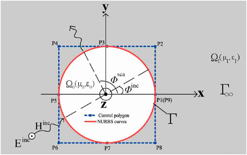
Figure 2. Sectional model boundary NURBS curve and control point.

First, we use the IGABEM/CFIE to calculate the RCS value at 800 MHz, $0<{\varphi }^{\text{sca}}<2\pi$, and back-scattering $\left({\varphi }^{\text{inc}}=0\right)$. The comparison between the result and the analytical solution is shown in Figure 3A. The figure shows that the analytical solution is very consistent with that of the IGABEM/CFIE. In addition, the RCS value begins to fluctuate when the scattering angle reaches 135° and reaches a maximum when the scattering angle reaches 180°.

Figure 3

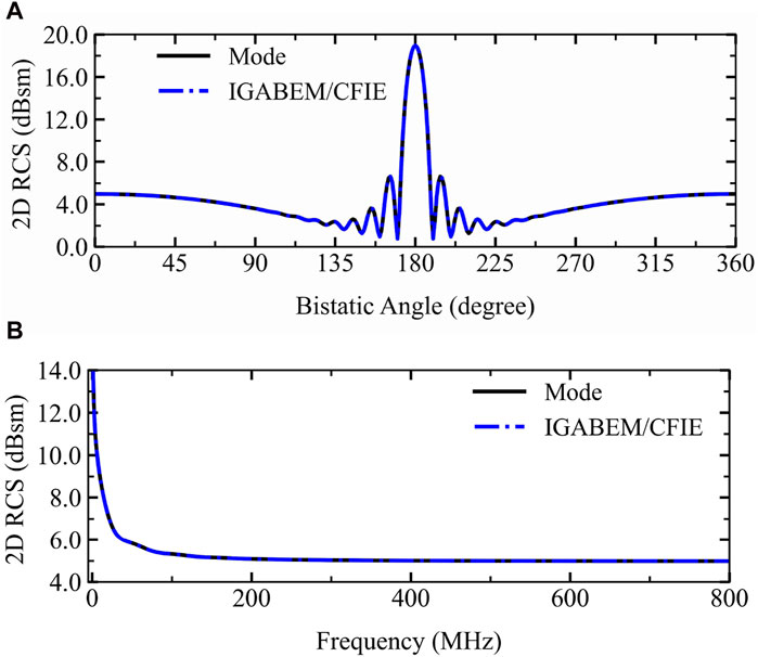
Figure 3. The RCS for PEC cylinder. (A) The RCS at 800 MHz under back-scattering. (B) The RCS at ϕ^inc = 0 at different frequency.

In addition, because of the symmetry of the example itself, its RCS is also symmetric at approximately 180°. Then, the IGABEM/CFIE is used to calculate the RCS value of the back-scattering at different frequencies. Figure 3B shows that its RCS gradually decreases with the change in frequency, and the final region is stable.In addition, the current at ${\varphi }^{\text{inc}}=0$ at 800 MHz is also calculated, and its absolute value, real part, and imaginary part are compared with the analytical solution, as shown in Figure 4. As can be seen, the IGABEM/CFIE is still in good agreement with the analytic solution. Furthermore, it can be seen that the current fluctuates greatly on both sides, and the fluctuation is small near ${\varphi }^a=\pi$ degrees, and the current is almost zero.

Figure 4

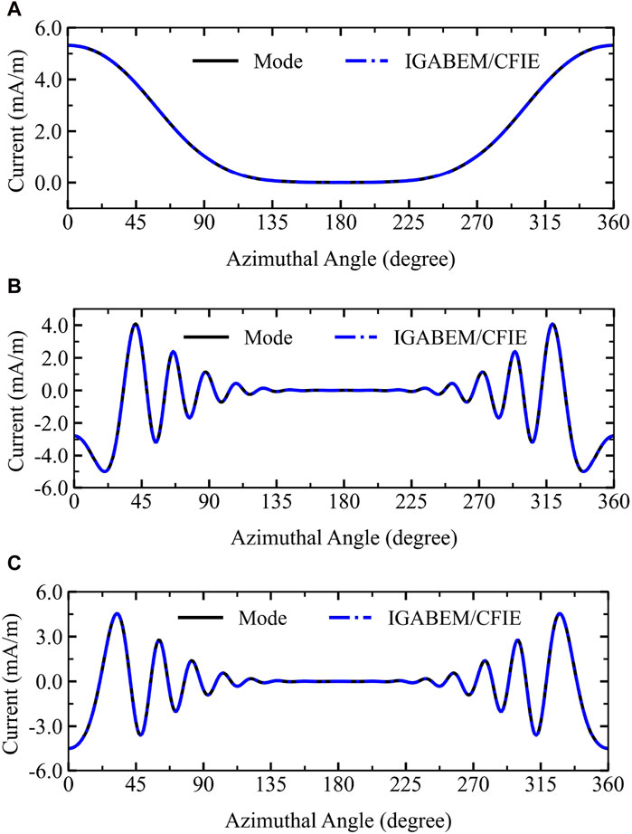
Figure 4. Current for the cylinder at 800 MHz with ${\varphi }^{\text{inc}}=0$. (A) $|\mathrm{J}\mathrm{z}(\mathrm{\varphi }\mathrm{a})|$; (B) $\mathrm{R}\mathrm{e}\mathrm{J}\mathrm{z}(\mathrm{\varphi }\mathrm{a})$; and (C) $\mathrm{I}\mathrm{m}\mathrm{J}\mathrm{z}(\mathrm{\varphi }\mathrm{a})$.

Finally, in order to observe the distribution of the electric field around the cylinder, we calculated the electric field near 20 × 20 m around the cylinder with ${\varphi }^{\text{inc}}=0$ at 800 MHz, as shown in Figure 5. It can be seen that the electric field is mainly distributed in the direction of the incident angle, and the direction of the incident angle is symmetrical.

Figure 5

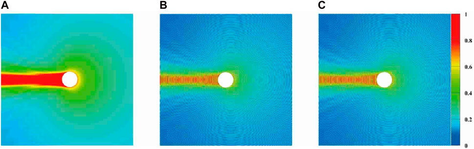
Figure 5. Electric field distribution around the PEC cylinder at 800 MHz: (A) ABS (Ez); (B) $\left|\mathrm{R}\mathrm{e}\left(\mathrm{E}\mathrm{z}\right)\right|$; and (C) $\left|\mathrm{I}\mathrm{m}\left(\mathrm{E}\mathrm{z}\right)\right|$.

In order to explore the sensitivity of the cylinder to shape change, we first calculated the sensitivity of the RCS scattered by the back-scattering at 800 MHz, $0\hspace{0.17em}⩽\hspace{0.17em}{\varphi }^{\text{sca}}\hspace{0.17em}⩽\hspace{0.17em}2\pi$, and compared the result with the analytical solution in Figure 6A; it can be seen that the IGABEM/CFIE still maintains a high coincidence. In addition, its RCS fluctuates more when ${\varphi }^{\text{sca}}=\pi$ but less on both sides. In addition, the sensitivity of RCS to shape change under back-scattering at different frequencies was calculated, as shown in Figure 6B. It can be seen that with the change in frequency, the RCS sensitivity gradually increases and eventually becomes stable.

Figure 6

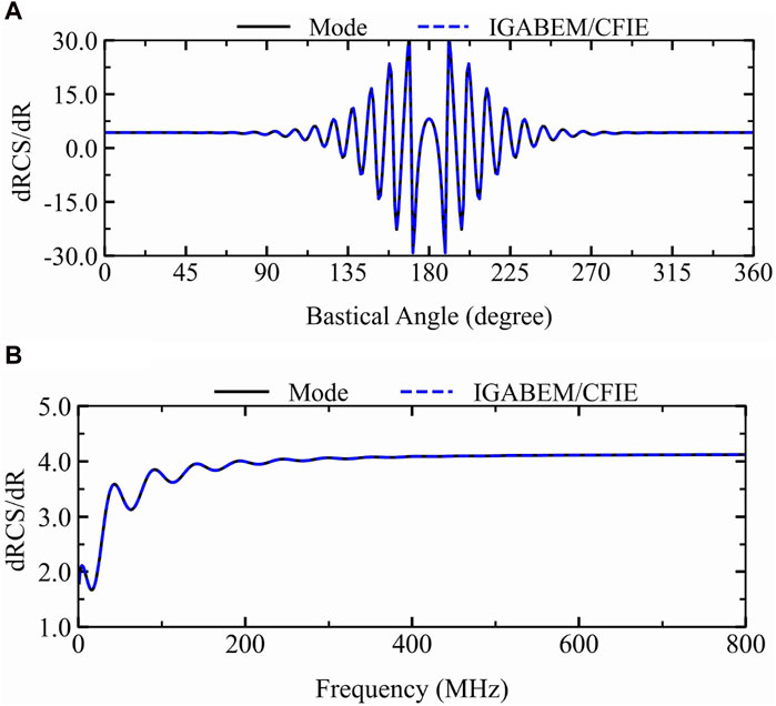
Figure 6. Sensitivity of RCS for the PEC cylinder to shape change: (A) RCS sensitivity at 800 MHz with ${\varphi }^{\text{inc}}=0$. (B) RCS sensitivity with ${\varphi }^{\text{inc}}=0$ at different frequencies.

In addition, the IGABEM/CFIE was used to calculate the sensitivity of the current to shape change at 800 MHz with ${\varphi }^{\text{inc}}=0$. The comparison results of the absolute value, real part, and imaginary part with the analytic solution are shown in Figure 7. It can be seen that the analytical solution is still very consistent with the IGABEM/CFIE. In addition, the current fluctuates greatly on both sides, and the sensitivity of the current is symmetric about ${\varphi }^a=\pi$.

Figure 7

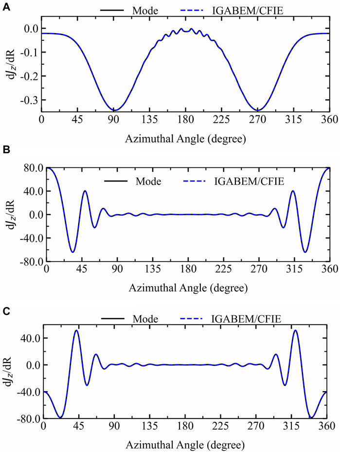
Figure 7. Sensitivity of the current for the PEC cylinder to shape change: (A) $|\mathrm{J}\mathrm{z}(\mathrm{\varphi }\mathrm{a})|$; (B) $\mathrm{R}\mathrm{e}\mathrm{J}\mathrm{z}(\mathrm{\varphi }\mathrm{a})$; and (C) $\mathrm{I}\mathrm{m}\mathrm{J}\mathrm{z}(\mathrm{\varphi }\mathrm{a})$.

Finally, in order to observe the sensitivity distribution of the electric field to shape change within the range of 20 × 20 around the cylinder, the sensitivity of the electric field to shape change under back-scattering at 800 MHz was calculated, as shown in Figure 8. It can be seen that the electric field is more sensitive to the shape change in the direction of the incident angle, and the remaining regions are almost zero. In addition, the direction of the incidence angle is symmetrical.

Figure 8

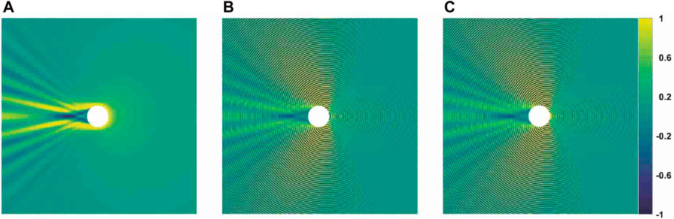
Figure 8. Sensitivity of the electric field around the cylinder to shape changes at 800 MHz ${\varphi }^{\text{inc}}=0$ TE polarization: (A) $\mathrm{A}\mathrm{b}\mathrm{s}\left(\mathrm{E}\mathrm{z}\right)/\mathrm{d}\mathrm{R}$; (B) $\left|\mathrm{R}\mathrm{e}\left(\mathrm{E}\mathrm{z}\right)\right|/\mathrm{d}\mathrm{R}$; and (C) $\left|\mathrm{I}\mathrm{m}\left(\mathrm{E}\mathrm{z}\right)\right|/\mathrm{d}\mathrm{R}$.

4.2 Deformation circle model

The deformation circle model is suitable for studying the shape change of objects under the action of external forces and is usually used in structural mechanics and civil engineering fields. In this section, we construct a deformation circle model by changing the location of control points $p2$, $p4$, $p6$, and $p8$ in Figure 2, as shown in Figure 9. Due to the particularity of the deformation circle, we explore the model from two perspectives ${\varphi }^{\text{inc}}=0$ and ${\varphi }^{\text{inc}}=45$.

Figure 9

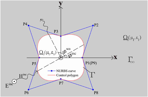
Figure 9. NURBS curve and control points of a deformation circle model.

First, we calculate the current at ${\varphi }^{\text{inc}}=0$ and ${\varphi }^{\text{inc}}=45$ at 800 MHz using the IGABEM/CFIE. As shown in Figure 10, when ${\varphi }^{\text{inc}}=0$, the current fluctuates greatly on both sides and is smaller when $90<{\varphi }^a<270$. When ${\varphi }^{\text{inc}}=45$, the current also fluctuates greatly on both sides, and it fluctuates less when $150<{\varphi }^a<300$.

Figure 10

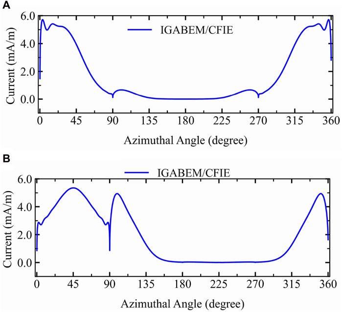
Figure 10. Current for the deformation circle model: (A) current at ${\varphi }^{\text{inc}}=0.$ (B) Current at ${\varphi }^{\text{inc}}=45$. (A) $|\mathrm{J}\mathrm{z}(\mathrm{\varphi }\mathrm{a})|$ and (B) $|\mathrm{J}\mathrm{z}(\mathrm{\varphi }\mathrm{a})|$.

In order to clearly observe the electric field distribution in the 20 × 20 region around the deformation circle model, the electric field distribution under ${\varphi }^{\text{inc}}=45$ at 800 MHz was also calculated, as shown in Figure 11. It can be seen that the electric field is more densely distributed in the direction of the incident angle and smaller in the other regions.

Figure 11

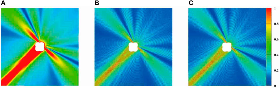
Figure 11. Electric field distribution around the PEC cylinder at 800 MHz: (A) ABS (Ez); (B) $\left|\mathrm{R}\mathrm{e}\left(E\mathrm{z}\right)\right|$; and (C) $\left|\mathrm{I}\mathrm{m}\left(\mathrm{E}\mathrm{z}\right)\right|$.

In addition, in order to explore the current sensitivity to shape change, we also calculated the current sensitivity to shape change at 800 MHz, ${\varphi }^{\text{inc}}=0$, and ${\varphi }^{\text{inc}}=45$. As shown in Figure 12, when ${\varphi }^{\text{inc}}=0$, the current fluctuates greatly on both sides, while the current fluctuates slightly when $120<{\varphi }^a<250$. In addition, due to the unique symmetry of the model, its current sensitivity is also symmetric about ${\varphi }^a=\pi$. When ${\varphi }^{\text{inc}}=45$, the current fluctuates more on both sides and less at $150<{\varphi }^a<290$. In addition, due to the unique symmetry of the example, $0<{\varphi }^a<90$ is symmetric with respect to ${\varphi }^a=45$. $90<{\varphi }^a<360$ is symmetric between ${\varphi }^a=225$.

Figure 12

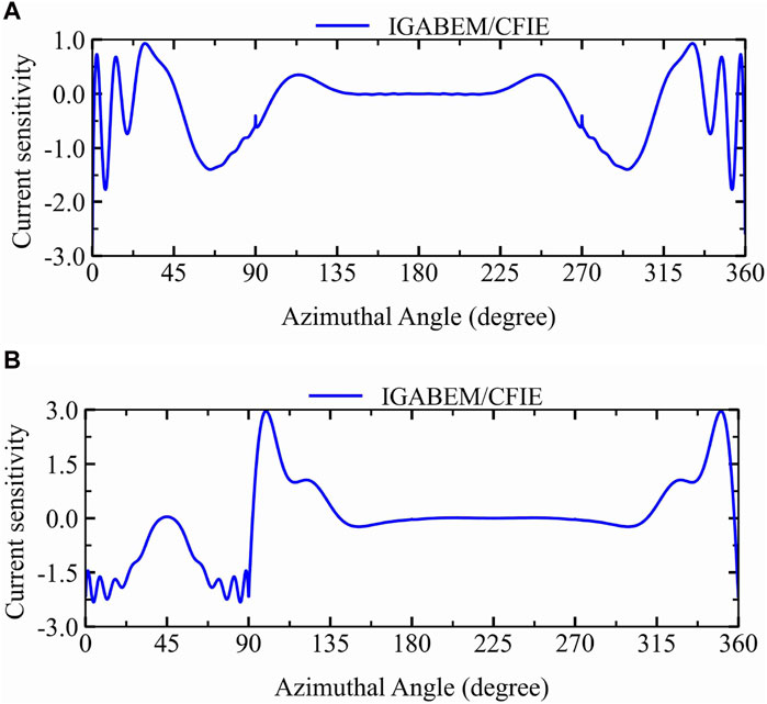
Figure 12. Sensitivity of the current to shape change: (A) current sensitivity with ${\varphi }^{\mathrm{i}\mathrm{n}\mathrm{c}}\hspace{0.17em}=\hspace{0.17em}0$. (B) Current sensitivity with ${\varphi }^{\mathrm{i}\mathrm{n}\mathrm{c}}\hspace{0.17em}=\hspace{0.17em}45$. (A) $|(\mathrm{\varphi }\mathrm{a})|$ sensitivity and (B) $|\mathrm{J}\mathrm{z}(\mathrm{\varphi }\mathrm{a})|$ sensitivity.

Finally, in order to better observe the sensitivity of the electric field around the deformation circle model to shape change, we calculated the sensitivity of the electric field to shape change at 800 MHz when ${\varphi }^{\text{inc}}=0$ in the surrounding 20 × 20 region, as shown in Figure 13. As shown in the figure, the electric field is relatively dense at the rear of the model, and because of the inherent symmetry of the deformation circle model, its electric field distribution is symmetrical with respect to the incident angle.

Figure 13

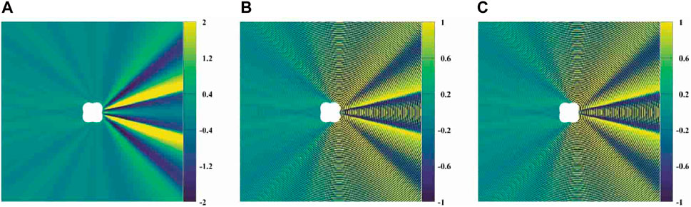
Figure 13. Sensitivity of the electric field around the model to shape change at 800 MHz: (A) Abs (Ez) sensitivity; (B) $\left|\mathrm{R}\mathrm{e}\left(\mathrm{E}\mathrm{z}\right)\right|$ sensitivity; and (C) $\left|\mathrm{I}\mathrm{m}\left(\mathrm{E}\mathrm{z}\right)\right|$ sensitivity.

5 Conclusion

In this paper, a formula that can be used to calculate two-dimensional electromagnetic scattering analysis is proposed by combining equal geometry and boundary elements, and then, a formula for electromagnetic scattering shape sensitivity analysis is proposed on the basis of the formula, which can provide reliable data guidance for sensitivity analysis and model optimization. Finally, two calculation columns are used to verify the effectiveness of the proposed method.

In future studies, we will extend the proposed algorithm to solve three-dimensional electromagnetic problems, thereby further enhancing its generality and applicability in various engineering fields.

Data availability statement

The original contributions presented in the study are included in the article/Supplementary Material; further inquiries can be directed to the corresponding author.

Author contributions

QH: writing–review and editing. CL: writing–original draft.

Funding

The author(s) declare that no financial support was received for the research, authorship, and/or publication of this article.

Conflict of interest

The authors declare that the research was conducted in the absence of any commercial or financial relationships that could be construed as a potential conflict of interest.

Publisher’s note

All claims expressed in this article are solely those of the authors and do not necessarily represent those of their affiliated organizations, or those of the publisher, the editors, and the reviewers. Any product that may be evaluated in this article, or claim that may be made by its manufacturer, is not guaranteed or endorsed by the publisher.

References

1. Rao S, Wilton D, Glisson A. Electromagnetic scattering by surfaces of arbitrary shape. IEEE Trans Antennas Propagation (1982) 30:409–18. doi:10.1109/tap.1982.1142818

CrossRef Full Text | Google Scholar

2. Jin JM The finite element method in electromagnetics. John Wiley and Sons (2015).

Google Scholar

3. Zhang G, He Z, Qin J, Hong J. Magnetically tunable bandgaps in phononic crystal nanobeams incorporating microstructure and flexoelectric effects. Appl Math Model (2022) 111:554–66. doi:10.1016/j.apm.2022.07.005

CrossRef Full Text | Google Scholar

4. Gibson WC The method of moments in electromagnetics. Chapman and Hall: CRC Press (2021).

Google Scholar

5. Taflove A, Hagness SC, Piket-May M Computational electromagnetics: the finite-difference time-domain method, vol. 3. Amsterdam, The Netherlands: Elsevier (2005).

Google Scholar

6. Chen J, Qu Y, Guo Z, Li D, Zhang G. A one-dimensional model for mechanical coupling metamaterials using couple stress theory. Math Mech Sol (2023) 28:2732–55. doi:10.1177/10812865231177670

CrossRef Full Text | Google Scholar

7. Qu Y, Pan E, Zhu FRAK, Jin F, Roy AK. Modeling thermoelectric effects in piezoelectric semiconductors: new fully coupled mechanisms for mechanically manipulated heat flux and refrigeration. Int J Eng Sci (2023) 182:103775. doi:10.1016/j.ijengsci.2022.103775

CrossRef Full Text | Google Scholar

8. Shen X, Du C, Jiang S, Zhang P, Chen L. Multivariate uncertainty analysis of fracture problems through model order reduction accelerated sbfem. Appl Math Model (2024) 125:218–40. doi:10.1016/j.apm.2023.08.040

CrossRef Full Text | Google Scholar

9. Liu Z, Bian P, Qu Y, Huang W, Chen L, Chen J, et al. A galerkin approach for analysing coupling effects in the piezoelectric semiconducting beams. Eur J Mech/A Sol (2024) 103:105145. doi:10.1016/j.euromechsol.2023.105145

CrossRef Full Text | Google Scholar

10. Chen L, Liu C, Zhao W, Liu L. An isogeometric approach of two dimensional acoustic design sensitivity analysis and topology optimization analysis for absorbing material distribution. Comput Methods Appl Mech Eng (2018) 336:507–32. doi:10.1016/j.cma.2018.03.025

CrossRef Full Text | Google Scholar

11. Chen L, Lian H, Dong H, Yu P, Jiang S, Bordas S. Broadband topology optimization of three-dimensional structural-acoustic interaction with reduced order isogeometric fem/bem. J Comput Phys (2024) 113051. doi:10.1016/j.jcp.2024.113051

CrossRef Full Text | Google Scholar

12. Nikolova NK, Li Y, Li Y, Bakr MH. Sensitivity analysis of scattering parameters with electromagnetic time-domain simulators. IEEE Trans microwave Theor Tech (2006) 54:1598–610. doi:10.1109/TMTT.2006.871350

CrossRef Full Text | Google Scholar

13. Sargheini S Shape sensitivity analysis of electromagnetic scattering problems. Ph.D. thesis. ETH Zurich (2016).

Google Scholar

14. Spies BR, Habashy TM. Sensitivity analysis of crosswell electromagnetics. Geophysics (1995) 60:834–45. doi:10.1190/1.1443821

CrossRef Full Text | Google Scholar

15. Kucherenko S, Rodriguez-Fernandez M, Pantelides C, Shah N. Monte Carlo evaluation of derivative-based global sensitivity measures. Reliability Eng Syst Saf (2009) 94:1135–48. doi:10.1016/j.ress.2008.05.006

CrossRef Full Text | Google Scholar

16. Jumabekova A, Berger J, Foucquier A. An efficient sensitivity analysis for energy performance of building envelope: a continuous derivative based approach. Building Simulation (2021) 14:909–30. doi:10.1007/s12273-020-0712-4

CrossRef Full Text | Google Scholar

17. Prabhakar Y. A combinatorial approach to the variable selection in multiple linear regression: Analysis of selwood et al. data set – a case study. Qsar Comb Sci (2010) 22:583–95. doi:10.1002/qsar.200330814

CrossRef Full Text | Google Scholar

18. Montgomery DC, Peck EA, Vining GG Introduction to linear regression analysis. John Wiley and Sons (2021).

Google Scholar

19. Seber GA, Lee AJ Linear regression analysis. John Wiley and Sons (2012).

Google Scholar

20. Maus S. Variogram analysis of magnetic and gravity data. Geophysics (2012) 64:776–84. doi:10.1190/1.1444587

CrossRef Full Text | Google Scholar

21. Bohling G. Introduction to geostatistics and variogram analysis. Kans Geol Surv (2005) 1:1–20.

Google Scholar

22. Raviart P-A, Thomas JM. A mixed finite element method for 2-nd order elliptic problems. In: Mathematical aspects of finite element methods (2006).

CrossRef Full Text | Google Scholar

23. Nguyen VP, Anitescu C, Bordas SP, Rabczuk T. Isogeometric analysis: an overview and computer implementation aspects. Mathematics Comput Simulation (2015) 117:89–116. doi:10.1016/j.matcom.2015.05.008

CrossRef Full Text | Google Scholar

24. Cottrell JA, Hughes TJ, Bazilevs Y Isogeometric analysis: toward integration of CAD and FEA. John Wiley and Sons (2009).

Google Scholar

25. Cottrell J, Hughes T, Reali A. Studies of refinement and continuity in isogeometric structural analysis. Comput Methods Appl Mech Eng (2007) 196:4160–83. doi:10.1016/j.cma.2007.04.007

CrossRef Full Text | Google Scholar

26. Fischer P, Klassen M, Mergheim J, Steinmann P, Müller R. Isogeometric analysis of 2d gradient elasticity. Comput Mech (2011) 47:325–34. doi:10.1007/s00466-010-0543-8

CrossRef Full Text | Google Scholar

27. Makvandi R, Reiher JC, Bertram A, Juhre D. Isogeometric analysis of first and second strain gradient elasticity. Comput Mech (2018) 61:351–63. doi:10.1007/s00466-017-1462-8

CrossRef Full Text | Google Scholar

28. Qu Y, Zhang G, Gao X-L, Jin F. A new model for thermally induced redistributions of free carriers in centrosymmetric flexoelectric semiconductor beams. Mech Mater (2022) 171:104328. doi:10.1016/j.mechmat.2022.104328

CrossRef Full Text | Google Scholar

29. Zhang G, Qu Y, Gao X-L, Jin F. A transversely isotropic magneto-electro-elastic timoshenko beam model incorporating microstructure and foundation effects. Mech Mater (2020) 149:103412. doi:10.1016/j.mechmat.2020.103412

CrossRef Full Text | Google Scholar

30. Li W, Ambati M, Nguyen-Thanh N, Du H, Zhou K. Adaptive fourth-order phase-field modeling of ductile fracture using an isogeometric-meshfree approach. Comput Methods Appl Mech Eng (2023) 406:115861. doi:10.1016/j.cma.2022.115861

CrossRef Full Text | Google Scholar

31. Shen X, Du C, Jiang S, Sun L, Chen L. Enhancing deep neural networks for multivariate uncertainty analysis of cracked structures by pod-rbf. Theor Appl Fracture Mech (2023) 125:103925. doi:10.1016/j.tafmec.2023.103925

CrossRef Full Text | Google Scholar

32. De Luycker E, Benson DJ, Belytschko T, Bazilevs Y, Hsu MC. X-fem in isogeometric analysis for linear fracture mechanics. Int J Numer Methods Eng (2011) 87:541–65. doi:10.1002/nme.3121

CrossRef Full Text | Google Scholar

33. Sun F, Dong C, Yang H. Isogeometric boundary element method for crack propagation based on bézier extraction of nurbs. Eng Anal Boundary Elem (2019) 99:76–88. doi:10.1016/j.enganabound.2018.11.010

CrossRef Full Text | Google Scholar

34. Khajah T, Antoine X, Bordas S Isogeometric finite element analysis of time-harmonic exterior acoustic scattering problems (2016). arXiv preprint arXiv:1610.01694.

Google Scholar

35. Chen L, Cheng R, Li S, Lian H, Zheng C, Bordas SPA. A sample-efficient deep learning method for multivariate uncertainty qualification of acoustic–vibration interaction problems. Comput Methods Appl Mech Eng (2022) 393:114784. doi:10.1016/j.cma.2022.114784

CrossRef Full Text | Google Scholar

36. Lu C, Chen L, Luo J, Chen H. Acoustic shape optimization based on isogeometric boundary element method with subdivision surfaces. Eng Anal Boundary Elem (2023) 146:951–65. doi:10.1016/j.enganabound.2022.11.010

CrossRef Full Text | Google Scholar

37. Zhang S, Yu B, Chen L. Non-iterative reconstruction of time-domain sound pressure and rapid prediction of large-scale sound field based on ig-drbem and pod-rbf. J Sound Vibration (2024) 573:118226. doi:10.1016/j.jsv.2023.118226

CrossRef Full Text | Google Scholar

38. Chen L, Zhang Y, Lian H, Atroshchenko E, Ding C, Bordas SP. Seamless integration of computer-aided geometric modeling and acoustic simulation: isogeometric boundary element methods based on catmull-clark subdivision surfaces. Adv Eng Softw (2020) 149:102879. doi:10.1016/j.advengsoft.2020.102879

CrossRef Full Text | Google Scholar

39. Chen L, Lian H, Liu Z, Chen H, Atroshchenko E, Bordas S. Structural shape optimization of three dimensional acoustic problems with isogeometric boundary element methods. Comput Methods Appl Mech Eng (2019) 355:926–51. doi:10.1016/j.cma.2019.06.012

CrossRef Full Text | Google Scholar

40. Chen L, Zhao J, Lian H, Yu B, Atroshchenko E, Pei L. A bem broadband topology optimization strategy based on taylor expansion and soar method—application to 2d acoustic scattering problems. Int J Numer Methods Eng (2023) 124:5151–82. doi:10.1002/nme.7345

CrossRef Full Text | Google Scholar

41. Chen L, Lian H, Liu Z, Gong Y, Zheng C, Bordas S. Bi-material topology optimization for fully coupled structural-acoustic systems with isogeometric fem–bem. Eng Anal Boundary Elem (2022) 135:182–95. doi:10.1016/j.enganabound.2021.11.005

CrossRef Full Text | Google Scholar

42. Chen L, Lian H, Natarajan S, Zhao W, Chen X, Bordas S. Multi-frequency acoustic topology optimization of sound-absorption materials with isogeometric boundary element methods accelerated by frequency-decoupling and model order reduction techniques. Comput Methods Appl Mech Eng (2022) 395:114997. doi:10.1016/j.cma.2022.114997

CrossRef Full Text | Google Scholar

43. Chen L, Lu C, Lian H, Liu Z, Zhao W, Li S, et al. Acoustic topology optimization of sound absorbing materials directly from subdivision surfaces with isogeometric boundary element methods. Comput Methods Appl Mech Eng (2020) 362:112806. doi:10.1016/j.cma.2019.112806

CrossRef Full Text | Google Scholar

44. Zhang M, Sun J, Chen W. An interface tracking method of coupled youngs-vof and level set based on geometric reconstruction. Chin J Theor Appl Mech (2019) 51:775–86.

Google Scholar

45. Takizawa K, Bazilevs Y, Tezduyar TE. Isogeometric discretization methods in computational fluid mechanics. Math Models Methods Appl Sci (2022) 32:2359–70. doi:10.1142/s0218202522020018

CrossRef Full Text | Google Scholar

46. Nørtoft P, Gravesen J. Isogeometric shape optimization in fluid mechanics. Struct Multidisciplinary Optimization (2013) 48:909–25. doi:10.1007/s00158-013-0931-8

CrossRef Full Text | Google Scholar

47. Hamdia KM, Ghasemi H, Zhuang X, Rabczuk T. Multilevel Monte Carlo method for topology optimization of flexoelectric composites with uncertain material properties. Eng Anal Boundary Elem (2022) 134:412–8. doi:10.1016/j.enganabound.2021.10.008

CrossRef Full Text | Google Scholar

48. Chen L, Li H, Guo Y, Chen P, Elena A, Lian H. Uncertainty quantification of mechanical property of piezoelectric materials based on isogeometric stochastic fem with generalized nth-order perturbation. Eng Comput (2023) 40:257–77. doi:10.1007/s00366-023-01788-w

CrossRef Full Text | Google Scholar

49. Qu Y, Zhu F, Pan E, Jin F, Hirakata H. Analysis of wave-particle drag effect in flexoelectric semiconductor plates via mindlin method. Appl Math Model (2023) 118:541–55. doi:10.1016/j.apm.2023.01.040

CrossRef Full Text | Google Scholar

50. Zhang G, Guo Z, Qu Y, Mi C. Global and local flexotronic effects induced by external magnetic fields in warping of a semiconducting composite fiber. Compos Structures (2022) 295:115711. doi:10.1016/j.compstruct.2022.115711

CrossRef Full Text | Google Scholar

51. Li H, Chen L, Zhi G, Meng L, Lian H, Liu Z, et al. A direct fe2 method for concurrent multilevel modeling of piezoelectric materials and structures. Comput Methods Appl Mech Eng (2024) 420:116696. doi:10.1016/j.cma.2023.116696

CrossRef Full Text | Google Scholar

52. Zang Q, Liu J, Ye W, Lin G. Isogeometric boundary element for analyzing steady-state heat conduction problems under spatially varying conductivity and internal heat source. Comput Math Appl (2020) 80:1767–92. doi:10.1016/j.camwa.2020.08.009

CrossRef Full Text | Google Scholar

53. Jahangiry HA, Jahangiri A. Combination of isogeometric analysis and level-set method in topology optimization of heat-conduction systems. Appl Therm Eng (2019) 161:114134. doi:10.1016/j.applthermaleng.2019.114134

CrossRef Full Text | Google Scholar

54. Yoon M, Ha S-H, Cho S. Isogeometric shape design optimization of heat conduction problems. Int J Heat Mass Transfer (2013) 62:272–85. doi:10.1016/j.ijheatmasstransfer.2013.02.077

CrossRef Full Text | Google Scholar

55. Cao G, Yu B, Chen L, Yao W. Isogeometric dual reciprocity BEM for solving non-Fourier transient heat transfer problems in FGMs with uncertainty analysis. Int J Heat Mass Transfer (2023) 203:123783. doi:10.1016/j.ijheatmasstransfer.2022.123783

CrossRef Full Text | Google Scholar

56. Qu Y, Jin F, Yang J. Effects of mechanical fields on mobile charges in a composite beam of flexoelectric dielectrics and semiconductors. J Appl Phys (2020) 127. doi:10.1063/5.0005124

CrossRef Full Text | Google Scholar

57. Qu Y, Zhou Z, Chen L, Lian H, Li X, Hu Z, et al. Uncertainty quantification of vibro-acoustic coupling problems for robotic manta ray models based on deep learning. Ocean Eng (2024) 299:117388. doi:10.1016/j.oceaneng.2024.117388

CrossRef Full Text | Google Scholar

58. Buffa A, Sangalli G, Vázquez R. Isogeometric analysis in electromagnetics: B-splines approximation. Comput Methods Appl Mech Eng (2010) 199:1143–52. doi:10.1016/j.cma.2009.12.002

CrossRef Full Text | Google Scholar

59. Buffa A, Sangalli G, Vázquez R. Isogeometric methods for computational electromagnetics: B-spline and t-spline discretizations. J Comput Phys (2014) 257:1291–320. doi:10.1016/j.jcp.2013.08.015

CrossRef Full Text | Google Scholar

60. Evans JA, Hughes TJ. Isogeometric divergence-conforming b-splines for the Darcy–Stokes–brinkman equations. Math Models Methods Appl Sci (2013) 23:671–741. doi:10.1142/s0218202512500583

CrossRef Full Text | Google Scholar

61. Simpson RN, Liu Z, Vazquez R, Evans JA. An isogeometric boundary element method for electromagnetic scattering with compatible b-spline discretizations. J Comput Phys (2018) 362:264–89. doi:10.1016/j.jcp.2018.01.025

CrossRef Full Text | Google Scholar

62. Takahashi T, Hirai T, Isakari H, Matsumoto T. An isogeometric boundary element method for three-dimensional doubly-periodic layered structures in electromagnetics. Eng Anal Boundary Elem (2022) 136:37–54. doi:10.1016/j.enganabound.2021.11.020

CrossRef Full Text | Google Scholar

63. Chen L, Lian H, Xu Y, Li S, Liu Z, Atroshchenko E, et al. Generalized isogeometric boundary element method for uncertainty analysis of time-harmonic wave propagation in infinite domains. Appl Math Model (2023) 114:360–78. doi:10.1016/j.apm.2022.09.030

CrossRef Full Text | Google Scholar

64. Takahashi T, Matsumoto T. An application of fast multipole method to isogeometric boundary element method for laplace equation in two dimensions. Eng Anal boundary Elem (2012) 36:1766–75. doi:10.1016/j.enganabound.2012.06.004

CrossRef Full Text | Google Scholar

65. Chen L, Wang Z, Lian H, Ma Y, Meng Z, Li P, et al. Reduced order isogeometric boundary element methods for cad-integrated shape optimization in electromagnetic scattering. Comput Methods Appl Mech Eng (2024) 419:116654. doi:10.1016/j.cma.2023.116654

CrossRef Full Text | Google Scholar

Appendix A: Analytical solution

The analytical solution for the scattered electric field of an infinite perfectly electric cylinder with TE-polarized incident waves is

$E_z^s\left(\rho ,{\varphi }_{\mathit{sca}}\right)={\displaystyle \sum _{n=0}^{\infty }}{j}^n{c}_n{A}_n{H}_n^{\left(2\right)}\left(k_0\rho \right)\cos \left(n{\varphi }_{\mathit{sca}}\right),(\mathrm{A1})$

where $|E_z^i|=1$ for convenience, ${\varphi }_{sca}$ is the bistatic scattering angle, and $c_n=1$ for $n=0$, and $c_n=2$ otherwise. For the conducting cylinder, the coefficient $A_n$ is

$A_n=-\frac{J_n\left(k_0\alpha \right)}{H_n^{\left(2\right)}\left(k_0\alpha \right)},(\mathrm{A2})$

where $\alpha$ is the radius of the cylinder. The scattered far electric field is

$E_z^s\left(\rho ,{\varphi }_{\mathit{sca}}\right)=\sqrt{\frac{2}{\pi }}\frac{e^{-j\left(k_0\rho -\pi /4\right)}}{\sqrt{k_0\rho }}{\displaystyle \sum _{n=0}^{\infty }}{\left(-1\right)}^n{c}_n{A}_n\cos n{\varphi }_{\mathit{sca}}.(\mathrm{A3})$

The induced electric current $J_z\left({\varphi }_{\alpha }\right)$ is

$J_z\left({\varphi }_{\alpha }\right)=\frac{2}{\pi {\eta }^0{k}_{0}a}{\displaystyle \sum _{n=0}^{\infty }}\frac{{\left(j\right)}^n{c}_n\cos n{\varphi }_{\alpha }}{H_n^{\left(2\right)}\left(k_{0}a\right)},(\mathrm{A4})$

where ${\varphi }_{\alpha }$ is the azimuthal angle on the surface of the cylinder. The above formula is the analytical solution of the scattered electric field of the PEC under TE polarization.