Two-dimensional acoustic analysis using Taylor expansion-based boundary element method

The use of boundary elements in two-dimensional acoustic analysis is presented in this study, along with a detailed explanation of how to derive the final discrete equations from the fundamental fluctuation equations. In order to overcome the fictitious eigenfrequency problem that might arise during the examination of the external sound field, this work employs the Burton-Miller approach. Additionally, this work uses the Taylor expansion to extract the frequency-dependent component from the BEM function, which speeds up the computation and removes the frequency dependency of the system coefficient matrix. The effect of the radiated acoustic field generated by underwater structures’ on thin-walled structures such as submarines and ships is inspected in this work. Numerical examples verify the accuracy of the proposed method and the efficiency improvement.

1 Introduction

Water, as another common acoustic medium, has a much higher acoustic impedance than air, and the difference between it and the mechanical impedance of common structures is not so large as to be directly negligible. Therefore, the effect of the radiated acoustic field generated by the vibration of underwater structures on structures in general and on thin-walled structures such as submarines and ships in particular is usually difficult to be directly ignored. These structures are subject to significant vibration during underwater navigation. Structural vibration causes noise [1–5], which in turn affects [6] the surrounding environment, thus triggering the engineering requirements for noise reduction. The analysis of the noise problem is actually the acoustic analysis [7, 8]. In the past research, the acoustic problems are divided into the finite sound field problems (also called the internal sound field problems) [9–12] and the infinite sound field problems (also called the external sound field problems) [13–15]. For finite sound field or internal sound field problems, the finite element method (FEM) [16–18] has been effective in solving such problems and has been widely used in practical analysis. The analysis of the outer sound field problem is much more complex than the inner sound field, and the analysis of the infinite sound field [19, 20] leads to a drastic increase in the computational volume, which is difficult to bear. The boundary element method (BEM) [21–26], on the other hand, only needing to discretize the model on the boundary, while automatically satisfying the radiation conditions at infinity, is widely used in the analysis of external acoustic problems [27, 28]. Moreover, BEM is a semi-analytic method constructed on the basis of the basic solution, leading to a higher accuracy.

Although BEM has many advantages in acoustic analysis, it also has some drawbacks. The first one is the singularity problem, which leads to poor accuracy or even wrong results. Chen et al. [29–32] successfully applied the singular phase elimination technique to the discontinuous higher-order element and compared the accuracy performance of different elements. The second one is the fictitious eigenfrequency problem [33–36], and the main solutions to this problem are CHIEF method and Burton-Miller method [37–40]. In this paper, Burton-Miller is used to solve the fictitious eigenfrequency problem. The third one is the high memory requirement problem. The coefficient matrix formed using BEM [41–43] is a dense matrix with high memory requirement, which limits the application of BEM in large-scale problems. However, although the boundary element coefficient matrix is dense, it has the property of low rank. A series of fast methods [44–46] using low-rank decomposition have been proposed, including fast multipole method, H-matrix, adaptive cross approximation and some other fast algorithms, which could successfully reduce the computational volume and memory usage, making it possible to apply BEM on complex engineering problems [47–49]. The fourth one is the frequency dependent problem. Unlike FEM, the kernel function of BEM is frequency-dependent. The discrete formation of the coefficient matrix is influenced by frequency, necessitating its recalculation under each distinct frequency [50–52], leading to a sharp increase in the computational volume of the boundary element under frequency band analysis. In acoustic wideband analysis, researchers have developed some fast algorithms to enhance the efficiency of solving large-scale problems. The frequency-dependent terms are separated from the integration kernel using Taylor series expansions of sine and cosine functions [53–59], which reduces the workload and computational time of numerical integration. To mitigate the frequency dependence of the system coefficient matrix, this study uses the Taylor expansion to extract the frequency-dependent terms embedded within the product function of BEM. This approach is undertaken to eliminate the influence of frequency variations on the matrix, thereby enhancing the accuracy and versatility of BEM [60–63] in diverse engineering applications.

In this paper, we introduce the Burton-Miller method and the Taylor expansion technique through two examples of circular and airfoil models. These two techniques solve the problem of spurious peaks present in the boundary element method and eliminate the influence of frequency variations on the matrix, thereby enhancing the accuracy and versatility of BEM. This provides a reference value for the study of underwater noise problems. In the course of this study we found that no spurious peaks occur when the radius of the circle is small. In the process of Taylor expansion, the magnitude of the error in the analytical solution and Taylor expansion is related to the number of expansion terms.

The following is the article’s remaining content: Using the Burton-Miller approach and the Taylor expansion series, the two-dimensional acoustic boundary element method is introduced in Section 2. Sections 3 offers numerical examples to back up the recommended method. Section 4 brings the text’s conclusions to a close.

2 Two-dimensional acoustic boundary element method

Suppose there exists a circular region ${\mathrm{\Omega }}_y$, whose boundary is $L$. If the domain is filled with a homogeneous ideal fluid medium, the fluctuation equation for the sound pressure in this circular region is

${\nabla }^{2}P\left(x,t\right)-\frac{1}{c_f^2}\frac{{\partial }^{2}P\left(x,t\right)}{\partial t^2}=0,\forall x\in {\mathrm{\Omega }}_y(1)$

in which ${\nabla }^2$ represents the Laplace operator, $P\left(x,t\right)$ signifies the sound pressure at a specific point $x$ within the sound field at a particular time $t$, and $c_f$ denotes the wave speed. Assuming a simple harmonic sound field, the sound pressure can be formulated as

$P\left(x,t\right)=p\left(x\right)e^{-i\omega t}(2)$

where $p(x)$ denotes the time-independent sound pressure value in imaginary units $i=\sqrt{-1}$, and the angular frequencies $\omega =2\pi f$, $e^{-i\omega t}$ are time-dependent terms. Since sound waves exist in simple harmonic form in many cases, and since the Fourier transform can be used to convert the time-domain data into the result of superposition of different simple harmonic wave components, in this paper we only consider the steady-state simple harmonic sound field. Substituting Eq. 1 into Eq. 2, the Helmholtz control differential equation based on sound pressure is obtained as

${\nabla }^{2}p\left(x\right)+k^{2}p\left(x\right)=0,\forall x\in {\mathrm{\Omega }}_{\text{y}}(3)$

where $k=\frac{\omega }{c_f}$ denotes the wave number. Ultimately the two-dimensional sound field problem transforms into a problem of solving the partial differential Eq. 3, and therefore boundary conditions need to be considered. For the 2D sound field problem, there are three types of boundary conditions that are usually considered, as shown in Figure 1:

Figure 1

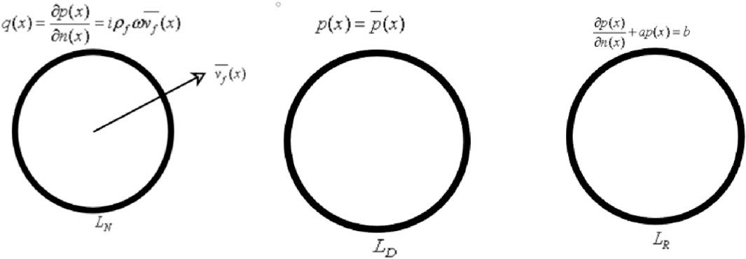
Figure 1. Schematic representation of the three boundary conditions.

Dirichlet boundary conditions, also known as Type I boundary conditions, where the sound pressure is known as Eq. 4

$p\left(x\right)=\bar{p}\left(x\right),\forall \mathrm{x}\in L_D(4)$

where $\overline{()}$ indicates that the value is known.

Neumann boundary conditions, also known as Type II boundary conditions, where the normal derivative of the sound pressure or the normal speed of vibration is known as Eq. 5

$q\left(x\right)=\frac{\partial p\left(x\right)}{\partial n\left(x\right)}=i{\rho }_y\omega \overline{v_y}\left(x\right),\forall x\in L_N(5)$

in which $q$ represents the acoustic flux, $n(x)$ signifies the external normal vector at point $x$, ${\rho }_y$ denotes the density of the acoustic medium, and $v_y$ represents the normal vibrational velocity of the acoustic medium at the boundary ${\mathrm{\Omega }}_y$, and the relationship between the acoustic flux and the normal vibrational velocity can be deduced from the Euler equation.

Robin boundary conditions, also known as Type III boundary conditions, where there is a certain linear relationship between the sound pressure and the derivative of sound pressure, as shown in Eq. 6

$\frac{\partial p\left(x\right)}{\partial n\left(x\right)}+ap\left(x\right)=b,\forall x\in L_R(6)$

where $a$ and $b$ are known coefficients.

2.1 Boundary integral equation

BEM is centered on the derivation of the boundary integral equation. By multiplying both ends of the Helmholtz equation by the weight function $A(x,y)$ and integrating over the sound field ${\mathrm{\Omega }}_{\text{y}}$, we get

${\int }_{{\mathrm{\Omega }}_y}\left[{\nabla }^{2}p\left(x\right)+k^{2}p\left(x\right)\right]A\left(x,y\right)d\mathrm{\Omega }\left(y\right)=0(7)$

Let the weight function $A(x,y)$ satisfy

${\nabla }^2\text{A}\left(\text{x},\text{y}\right)+{\mathrm{k}}^2\text{A}\left(\text{x},\text{y}\right)=-\delta \left(x-y\right)(8)$

when $x\in {\mathrm{\Omega }}_{\text{y}}$ and $x\notin L$, according to Eqs 7, 8, we get

${\int }_{{\mathrm{\Omega }}_y}p\left(y\right)\left[{\nabla }^2\text{A}\left(\text{x},\text{y}\right)+{\mathrm{k}}^2\text{A}\left(\text{x,\hspace{0.17em}y}\right)\right]d\mathrm{\Omega }\left(y\right)=-{\int }_{{\mathrm{\Omega }}_y}p\left(y\right)\delta \left(x-y\right)d\mathrm{\Omega }\left(y\right)=-p\left(x\right)(9)$

Equation 7 is transformed by Green’s second constant, and then Eq. 9 can be substituted to obtain the integral equation:

$p\left(x\right)+{\int }_{L}B\left(x,y\right)p\left(y\right)dL\left(y\right)={\int }_{L}A\left(x,y\right)q\left(y\right)dL\left(y\right)(10)$

where $q(y)=\frac{\partial p(y)}{\partial n(y)}$ denotes the sound flux. According to the above equation, the sound pressure at point $x$ can be regarded as the result of the superposition of the sound pressure and sound flux generated by the sound source point $y$. If the field point x is approximated to the integration boundary $L$, $x\in L$, Eq. 10 can be written as

$c\left(x\right)p\left(x\right)+{\int }_{L}B\left(x,y\right)p\left(y\right)dL\left(y\right)={\int }_{L}A\left(x,y\right)q\left(y\right)dL\left(y\right)(11)$

where the coefficient $c(x)$ depends on the geometric features at point $x$. Eq. 11 is known as the conventional boundary integral equation (CBIE). If the boundary at point $x$ is smooth, then $c(x)=1/2$. Derivation to the outer normal $n(x)$ yields the normal derivative boundary integral equation (NDBIE), as shown as

$c\left(x\right)q\left(x\right)+{\int }_{L}D\left(x,y\right)p\left(y\right)dL\left(y\right)={\int }_{L}E\left(x,y\right)q\left(y\right)dL\left(y\right)(12)$

The kernel function of each order in Eqs 11, 12 can be expressed as Eq. 13

$\begin{array}{ll}\hfill & A\left(x,y\right)=\frac{\mathrm{i}}{4}{H}_0^{\left(1\right)}\left(kr\right)\hfill \\ \hfill & B\left(x,y\right)=\frac{\partial A\left(x,y\right)}{\partial n\left(x\right)}=-\frac{\mathrm{i}k}{4}{H}_1^{\left(1\right)}\left(kr\right)\frac{\partial r}{\partial n\left(x\right)}\hfill \\ \hfill & E\left(x,y\right)=\frac{\partial A\left(x,y\right)}{\partial n\left(x\right)}=-\frac{\mathrm{i}k}{4}{H}_1^{\left(1\right)}\left(kr\right)\frac{\partial r}{\partial n\left(x\right)}\hfill \\ \hfill & D\left(x,y\right)=\frac{{\partial }^{2}A\left(x,y\right)}{\partial n\left(x\right)\partial n\left(y\right)}=\frac{\mathrm{i}k}{4r}{H}_1^{\left(1\right)}\left(kr\right)n_j\left(x\right)n_j\left(y\right)-\frac{\mathrm{i}{k}^2}{4}{H}_2^{\left(1\right)}\left(kr\right)\frac{\partial r}{\partial n\left(x\right)}\frac{\partial r}{\partial n\left(y\right)}\hfill \end{array}(13)$

where $r=\left|x-y\right|$ denotes the Euclidean distance between the field point and the source point, and $H_n^{(1)}$ denotes the nth order first class Hankel function.

When solving a two-dimensional sound field problem using Eq. 11 or Eq. 12 alone, there are some special frequencies where the computed results will deviate significantly from the analytical solution. However, these are only mathematical problems brought about by the use of boundary integral equations for solving the problem and do not have any real physical significance, and these frequencies are called fictitious eigenfrequencies. Although using either boundary integral equation alone may fail to obtain the correct solution at a particular frequency, a linear combination of Eqs 11, 12 gets an exact and unique solution, which is known as the Burton-Miller method. The combined form can be expressed as

$CBIE+\alpha NDBIE=0(14)$

where $\alpha$ denotes the coupling coefficient, $\alpha =i/k$ when the wave number $k\ge 1$, and vice versa $\alpha =i$.

Different element types can be used to discretize the boundary, and in order to facilitate the representation of the element types, a convention is adopted for the representation of the element types: CBEmn denotes a continuous element, m denotes m geometric interpolation points, and n denotes n physical interpolation points. The boundary is now discretized into a number of constant elements CBE21 since there is only one interpolation point in the element. A schematic diagram of the this element is shown in Figure 2.

Figure 2

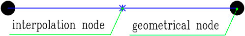
Figure 2. Schematic diagram of CBE21 element.

The boundary is now discretized into N constant elements, and the values of the physical quantities $p$ and $q$ on the elements are equal to the values of the interpolated nodes. For the integral of the $i$ node over the $j$ element, Eq. 11 can be discretized into the following form

$c\left(x\right)p^i+{\displaystyle \sum _{j=1}^N}{\int }_{L_j}B\left(x,y\right)dL\left(y\right)p^j={\displaystyle \sum _{j=1}^N}{\int }_{L_j}A\left(x,y\right)dL\left(y\right)q^j(15)$

in which ${\int }_{L_j}A(x,y)q(y)dL(y)$ and ${\int }_{L_j}B(x,y)p(y)dL(y)$ are both directly computable. Introducing the coefficient matrices $\mathbf{G}$ and $\mathbf{H}$, we have Eqs 16, 17

${\widehat{H}}^{ij}={\int }_{L_j}B\left(x,y\right)p\left(y\right)dL\left(y\right)(16)$

and

$G^{ij}={\int }_{L_j}A\left(x,y\right)q\left(y\right)dL\left(y\right)(17)$

Then Eq. 15 can be rewritten as

${\displaystyle \sum _{\mathrm{j}=1}^N}{H}^{ij}{p}^j={\displaystyle \sum _{\mathrm{j}=1}^N}{G}^{ij}{q}^j(18)$

If we assume that the boundary is smooth, then c(x) = 1/2, and $H^{ij}$ in Eq. 18 can be expressed as Eq. 19

$H^{ij}=\left\{\begin{array}{c}{\widehat{H}}^{ij},i\ne j\hfill \\ {\widehat{H}}^{ij}+\frac{1}{2},i=j\hfill \end{array}\right.(19)$

The same discretization can be performed on Eq. 12, and then according to Eq. 14 the matrix form of the linear system equations can be obtained as Eq. 20

$\mathbf{H}\mathbf{p}=\mathbf{G}\mathbf{q}(20)$

Reassembling Eq. 20 by moving all the unknowns to the left side of the equation and transferring all the knowns to the right side of the equation yields Eq. 21

$\mathbf{A}\mathbf{x}=\mathbf{b}(21)$

where $\mathbf{A}$ represents the asymmetric full-rank coefficient matrix, $\mathbf{x}$ denotes the unknown vector associated with the boundary nodes, and $\mathbf{b}$ signifies the known vector. By solving this equation, the unknown values at all nodes can be determined. Subsequently, the sound pressure ${\mathbf{P}}_y$ at any point within the domain can be calculated by substituting the obtained results into Eq. 22.

${\mathbf{P}}_y={\mathbf{G}}_y\mathbf{q}-{\mathbf{H}}_y\mathbf{p}(22)$

where ${\mathbf{H}}_y$ and ${\mathbf{G}}_y$ are the coefficient matrices when the field point y is in the outer acoustic domain.

2.2 Wideband analysis based on Taylor theory

The Green’s function $A(x,y)$ incorporates the $n$-th order Hankel function of the first kind, which exhibits an explicit dependence on the wave number $k$. The Taylor expansion of this Hankel function, centered at a designated frequency expansion point $z_0=k_{0}r$, can be formulated as Eq. 23

$H_n^{\left(1\right)}\left(z\right)={\displaystyle \sum _{m=0}^{\infty }}\frac{{\left(z-z_0\right)}^m}{m!}{\left[H_n^{\left(1\right)}\left(z\right)\right]}_{z=z_0}^{\left(m\right)}(23)$

where we have Eq. 24

${\left[H_n^{\left(1\right)}\left(z\right)\right]}_{z=z_0}^{\left(m\right)}=\frac{{\text{d}}^m{H}_n^{\left(1\right)}\left(z\right)}{\text{d}{z}^m}{|}_{z=z_0}(24)$

The Taylor expansion of the kernel functions presented in Eq. 23 can be analogously derived by substituting $z$ and $z_0$ with $kr$ and $k_{0}r$, respectively.

Note the considerable challenge in deriving an explicit expression for the $m$-th order derivative of the $n$-th order Hankel function, as presented in Eq. 23. To overcome this difficulty, a recursive formulation for the Hankel function is introduced as

$\frac{\text{d}{H}_n^{\left(1\right)}\left(z\right)}{\text{d}z}=\frac{n}{z}{H}_n^{\left(1\right)}\left(z\right)-H_{n+1}^{\left(1\right)}\left(z\right)(25)$

The recursive expression for the $m$-th order derivative of the $n$-th order Hankel function can be obtained through iterative differentiation of Eq. 25 with respect to the variable $z$. Specifically, this involves repeatedly applying the differentiation operator to obtain the desired derivative order, as shown in Eq. 26.

${\left[H_n^{\left(1\right)}\left(z\right)\right]}^{\left(m\right)}={\displaystyle \sum _{i=1}^m}{\left[H_n^{\left(1\right)}\left(z\right)\right]}^{\left(m-i\right)}\frac{{\left(-1\right)}^{i+1}\left(m-1\right)!}{z^i\left(m-i\right)!}-{\left[H_{n+1}^{\left(1\right)}\left(z\right)\right]}^{\left(m-1\right)}(26)$

By substituting Eq. 23 into Eqs 11, 12, then incorporating the impedance boundary condition $q(x)=i{\rho }_y\omega \overline{v_y}(x)$ to represent the sound absorption properties, the integrals in Eqs 11, 12 can be reformulated into an expansion form tailored to the fixed frequency point $k_0$:

$\begin{array}{c}{\int }_{L}B\left(x,y\right)p\left(y\right)dL\left(y\right)={\displaystyle \sum _{m=0}^{\infty }}\frac{{\left(k-k_0\right)}^m}{m!}{I}_1^m\hfill \\ {\int }_{L}A\left(x,y\right)q\left(y\right)dL\left(y\right)={\displaystyle \sum _{m=0}^{\infty }}\frac{{\left(k-k_0\right)}^m}{m!}{I}_2^m\hfill \\ \alpha {\int }_{L}D\left(x,y\right)p\left(y\right)dL\left(y\right)={\displaystyle \sum _{m=0}^{\infty }}\frac{{\left(k-k_0\right)}^m}{m!}\left(k{I}_3^m+k^2{I}_4^m\right)\hfill \\ \alpha {\int }_{L}E\left(x,y\right)q\left(y\right)dL\left(y\right)={\displaystyle \sum _{m=0}^{\infty }}\frac{{\left(k-k_0\right)}^m}{m!}k{I}_5^m\hfill \end{array}(27)$

where

$\begin{array}{c}{I}_1^m=-{\int }_L\frac{\mathrm{i}{r}^{m-1}}{4}{\left[z{H}_1^{\left(1\right)}\left(z\right)\right]}_{z=k_{0}r}^{\left(m\right)}\frac{\partial r}{\partial n\left(y\right)}p\left(y\right)d\left(y\right)\\ I_2^m={\int }_L\frac{i{r}^m}{4}{\left[H_0^{\left(1\right)}\left(z\right)\right]}_{z=k_{0}r}^{\left(m\right)}q\left(y\right)dL\left(y\right)\\ I_3^m={\int }_L\frac{\alpha \mathrm{i}{r}^{m-1}}{4}{\left[H_1^{\left(1\right)}\left(z\right)\right]}_{z=k_{0}r}^{\left(m\right)}{n}_j\left(x\right)n_j\left(y\right)p\left(y\right)dL\left(y\right)\\ I_4^m={\int }_L\frac{\alpha \mathrm{i}{r}^m}{4}{\left[H_2^{\left(1\right)}\left(z\right)\right]}_{z=k_{0}r}^{\left(m\right)}\frac{\partial r}{\partial n\left(x\right)}\frac{\partial r}{\partial n\left(y\right)}p\left(y\right)dL\left(y\right)\\ I_5^m=-{\int }_L\frac{\alpha \mathrm{i}{r}^m}{4}{\left[H_1^{\left(1\right)}\left(z\right)\right]}_{z=k_{0}r}^{\left(m\right)}\frac{\partial r}{\partial n\left(y\right)}q\left(y\right)dL\left(y\right)\end{array}(28)$

wherein, the $m$-th derivative of the function $z{H}_1^{(1)}(z)$ appearing in the integral $I_1^m$ can be calculated as Eq. 29

${\left[z{H}_1^{\left(1\right)}\left(z\right)\right]}^{\left(m\right)}=m{\left[H_1^{\left(1\right)}\left(z\right)\right]}^{\left(m-1\right)}+z{\left[H_1^{\left(1\right)}\left(z\right)\right]}^{\left(m\right)}(29)$

Substituting Eq. 27 into Eqs 11, 12 then simultaneously applying the impedance boundary condition $q(x)=i{\rho }_y\omega \overline{v_y}(x)$ yields the following result:

$C\left(x\right)\left[p\left(x\right)-q\left(x\right)\right]+{\displaystyle \sum _{m=0}^{\infty }}\frac{{\left(k-k_0\right)}^m}{m!}\left[\left(I_1^m-I_2^m\right)+\left(I_3^m-I_5^m\right)k+I_4^m{k}^2\right]=0(30)$

Owing to the presence of singular kernel functions and their normal derivatives in Eq. 14, the boundary integrals containing a sequence of expansion expressions in Eq. 28 exhibit singularities as well. These integrals are evaluated by employing the Cauchy principal value and the Hadamard finite part integral technique [64].

The discretization of Eq. 30 is achieved through the application of the collocation method, employing constant elements, which results in:

$\left[\mathbf{C}+{\displaystyle \sum _{m=0}^{\infty }}\frac{{\left(k-k_0\right)}^m}{m!}\left({\mathbf{I}}_1^m+k{\mathbf{I}}_3^m+k^2{\mathbf{I}}_4^m\right)\right]\mathbf{p}=\left[\alpha \mathbf{C}+{\displaystyle \sum _{m=0}^{\infty }}\frac{{\left(k-k_0\right)}^m}{m!}\left({\mathbf{I}}_2^m+k{\mathbf{I}}_5^m\right)\right]\mathbf{q}(31)$

where we have Eq. 32

$\mathbf{C}=\left[\begin{array}{ccc}\hfill C_1\hfill & \hfill \hfill & \hfill \mathbf{0}\hfill \\ \hfill \hfill & \hfill \ddots \hfill \\ \hfill \mathbf{0}\hfill & \hfill \hfill & \hfill C_N\hfill \end{array}\right](32)$

In the present study, we employ the Taylor expansion technique to decompose the frequency-dependent system matrix given in Eqs 11, 12 into a summation of frequency-dependent scalar functions multiplied by frequency-independent system matrices. Upon examination of Eq. 31, it becomes evident that the coefficients ${\mathbf{I}}_1^m,{\mathbf{I}}_2^m,{\mathbf{I}}_3^m,{\mathbf{I}}_4^m,{\mathbf{I}}_5^m$ exhibit no frequency dependence. Consequently, these coefficients need to be computed only once for multi-frequency problems, thereby eliminating the need for repeated computations. As a result, the coefficient matrix remains frequency-independent.

2.3 Symbols

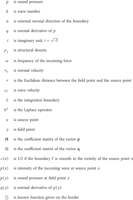
The following symbols are used in the formulas:

3 Numerical example

3.1 Cylindrical Shell’s 2-D cross section

Considering a infinitely long cylindrical shell pipe model, in which the radius is $r_0$, and the center of the circle is at (0, 0). Take the cross section of this cylindrical shell, then it is a two-dimensional problem. The normal velocity $v_0$ at the boundary of the cross section is randomly set to be a constant, $9.6\times 10^{-5}$ m/s. The boundary conditions are $q=i{\rho }_y\omega v_0$. The cross section is uniformly discretized into 100 constant elements. When the pipe radius $r_0$ is taken as 0.60 m …… 0.85 m, and the frequency $f$ is taken as 0–1,000 Hz (in step of 1 Hz), the sound pressure at point (2, 0) m is calculated here using CBIE and Burton-Miller, respectively. The results of sound pressure calculated using these two methods are shown in Figure 3.

Figure 3

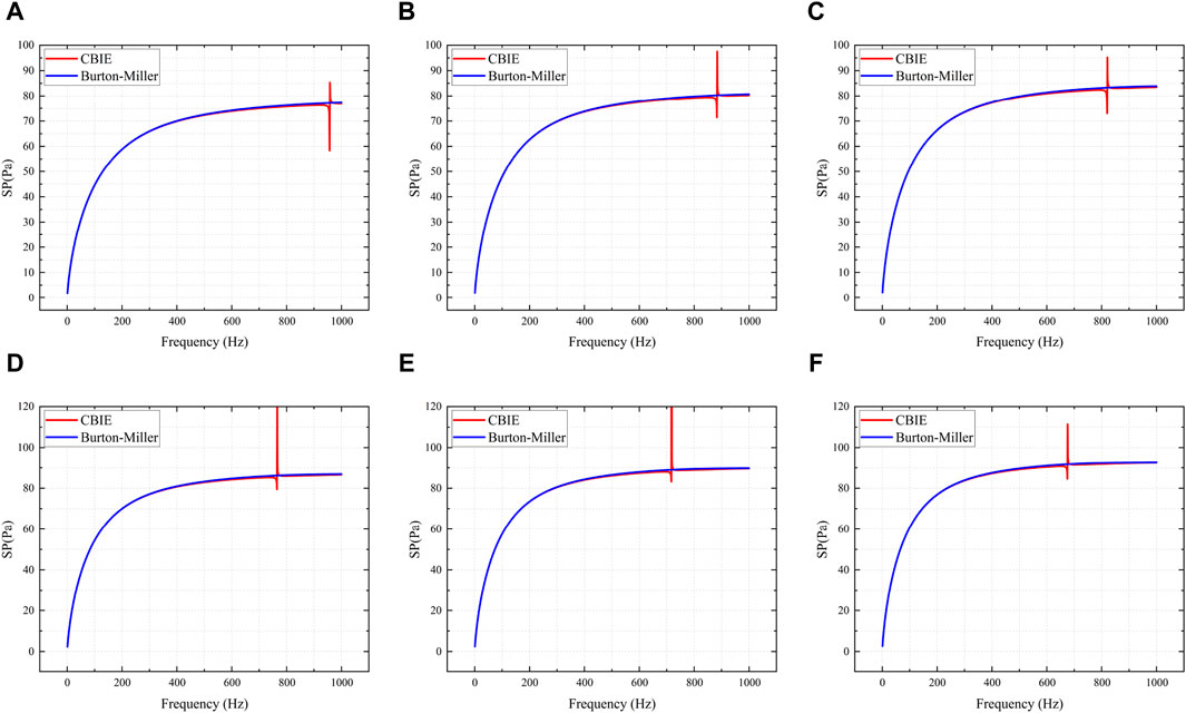
Figure 3. Sound pressure obtained using CBIE and Burton-Miller for different radius. (A): r₀ = 0.60 m, (B): r₀ = 0.65 m, (C): r₀ = 0.70 m, (D): r₀ = 0.75 m, (E): r₀ = 0.80 m, (F): r₀ = 0.85 m.

Several conclusions can be inferred from Figure 3. As the radius of the pipe increases, the sound pressure also increases. The results obtained using the conventional boundary element method (CBEM) and Burton-Miller exhibit a high degree of similarity. However, when the radius exceeds $0.60m$, CBEM tends to produce fictitious engenfrwquencies, whereas the Burton-Miller method proves effective in mitigating this issue.

The sound pressure results obtained using BEM based on Taylor expansion are presented in Figure 4. A frequency step of 1 Hz is utilized, and the width of each frequency band is set to $z$. The notation $Taylor\text{\_}3$ refers to the numerical solution derived using Taylor expansion with three expansion terms (TM = 3). Similarly, $Taylor\text{\_}5$, $Taylor\text{\_}7$, and $Taylor\text{\_}10$ represent the numerical solutions employing five, seven, and ten expansion terms, respectively.

Figure 4

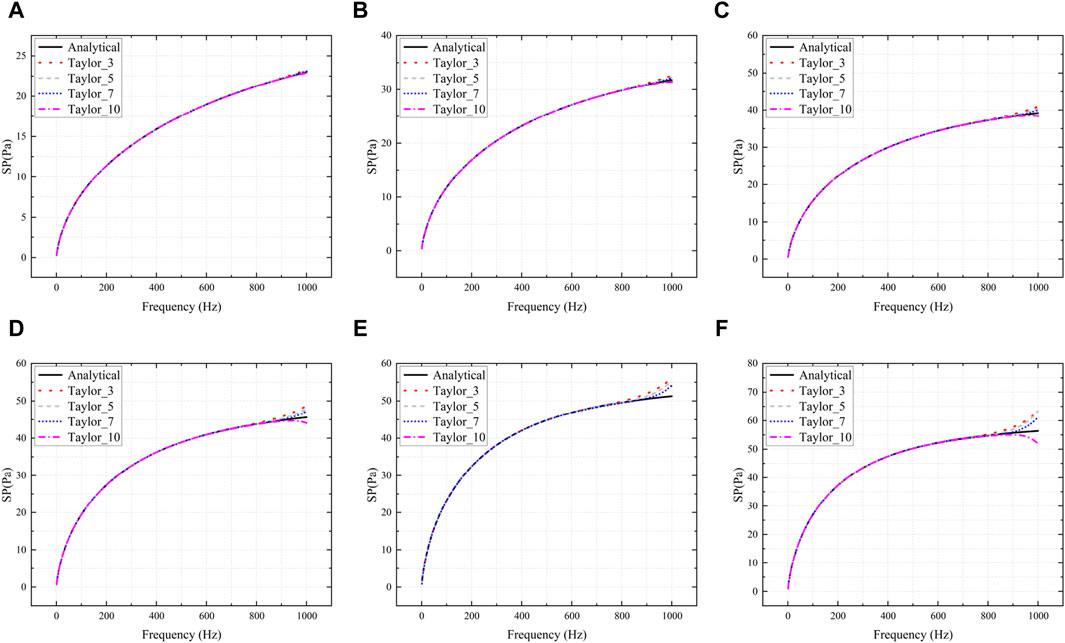
Figure 4. Sound pressure calculated with different number of Taylor expansion terms. (A): r₀ = 0.10 m, (B): r₀ = 0.15 m, (C): r₀ = 0.20 m, (D): r₀ = 0.25 m, (E): r₀ = 0.30 m, (F): r₀ = 0.35 m.

It becomes evident that sound pressure values exhibit variations across different frequency bands, as shown in Figure 4. Furthermore, within the same frequency band, the sound pressure values determined through the numerical method closely align with those obtained analytically. However, as the distance from the expansion point increases, the error also increases. Among the considered Taylor expansion terms, $Taylor\text{\_}10$ demonstrates the closest agreement with the sound pressure values obtained analytically. This implies that increasing the number of Taylor expansion terms leads to a numerical solution that more closely approximates the analytical solution.

As depicted in Figure 4, the numerical results exhibit general concordance with the analytical solution across various numbers of expansion terms. However, notable discrepancies arise at the extremities of the frequency band range. The observed agreement between the numerical and analytical solutions is primarily evident in the central region of the frequency spectrum. The discrepancies observed at the lower and upper ends of the frequency range primarily arise from the positioning of the fixed frequency expansion point at the midpoint of the range. As a result, as the distance from this fixed expansion point increases, the accuracy of the numerical results tends to deteriorate. To mitigate these deviations, the original frequency range of [1, 1,000] Hz has been subdivided into four distinct subranges: [1, 250] Hz, [250, 500] Hz, [500, 750] Hz, and [750, 1,000] Hz. Subsequent numerical simulations have been conducted within these refined subranges. As an illustrative example, consider the case where $r_0=0.40m$. As can be seen from Figure 5, by adopting this segmented approach, the accuracy and reliability of the numerical results are improved, particularly at the extremities of the frequency spectrum.

Figure 5

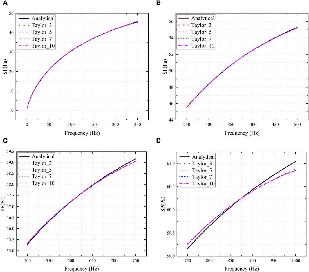
Figure 5. Sound pressure calculated with different number of Taylor expansion terms. $r_0$ = 0.40 m. (A): 1–250 Hz, (B): 250–500 Hz, (C): 500–750 Hz, (D): 750–1000 Hz.

The $\mathrm{C}\mathrm{P}\mathrm{U}$ time consumed using $\mathrm{C}\mathrm{B}\mathrm{I}\mathrm{E}$ and Taylor expansion is demonstrated in Figure 6. We can see that the former method takes much more time than the latter. Therefore, The decoupling method represented by Taylor expansion effectively reduces the time for wideband computation.

Figure 6

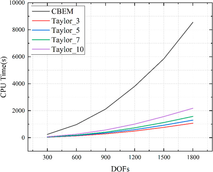
Figure 6. CPU time for different number of expansion terms.

3.2 Airfoil model

Due to the continuous development of artificial intelligence, bionic technology is becoming more and more sophisticated. Now we are working on the fins of an underwater bionic fish, which we can simplify into a wing-shaped model. For the airfoil model shown in Figure 7, CBIE and Taylor expansion is used to calculate the sound pressure at (2, 0) in the four frequency bands of [1–1,000] Hz, [1,000–2,000] Hz, [2,000–3,000] Hz and [3,000–4,000] Hz, respectively, as shown in Figure 8. It can be seen that the analytical solution bears a substantial resemblance to the solution derived using Taylor expansion across various frequency bands. Notably, the outcome at the Taylor expansion point precisely aligns with the analytical solution. However, as one moves further away from the expansion point, the divergence between the two solutions gradually increases.

Figure 7

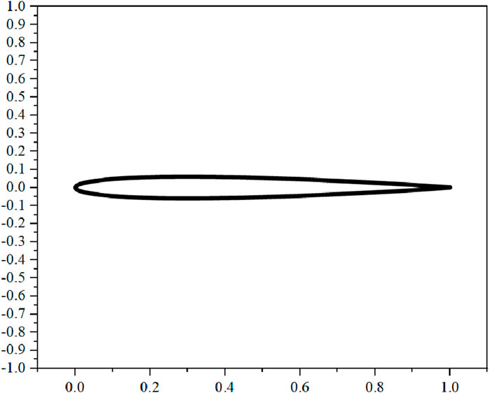
Figure 7. The airfoil Model.

Figure 8

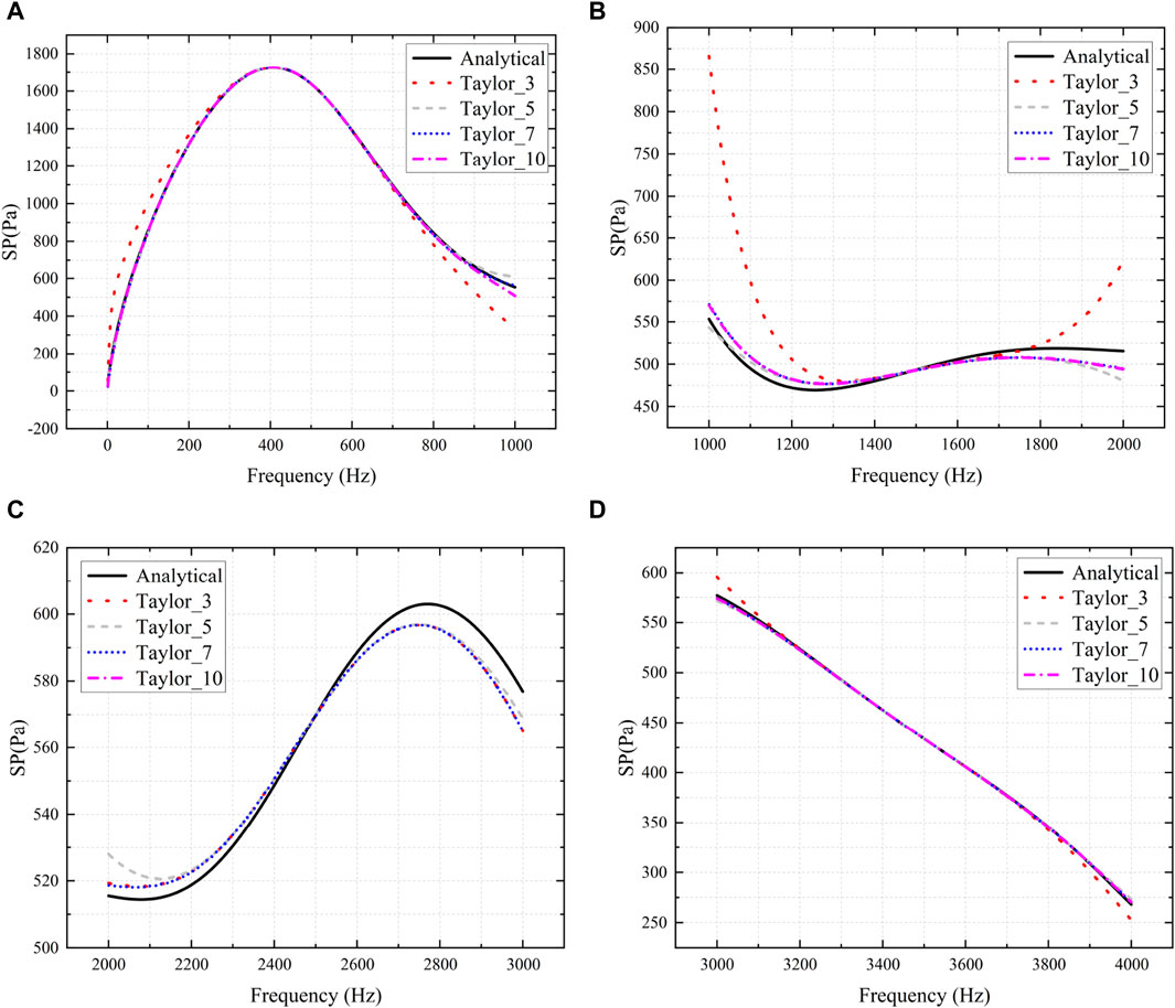
Figure 8. Sound pressure obtained using the analytical method and the boundary element method based on Taylor expansion. (A): 1–1000 Hz, (B): 1000–2000 Hz, (C): 2000–3000 Hz, (D): 3000–4000 Hz.

To minimize the errors arising from the calculation, we will continue to subdivide [1–1,000] Hz into [1–250] Hz, [250–500] Hz, [500–750] Hz and [750–1,000] Hz, as shown in Figure 9. It can be seen that as the frequency band decreases, the solution based on Taylor expansion results in smaller errors. Therefore, we can conclude that the smaller the frequency band of the expansion, the closer the result of the Taylor expansion is to the real solution.

Figure 9

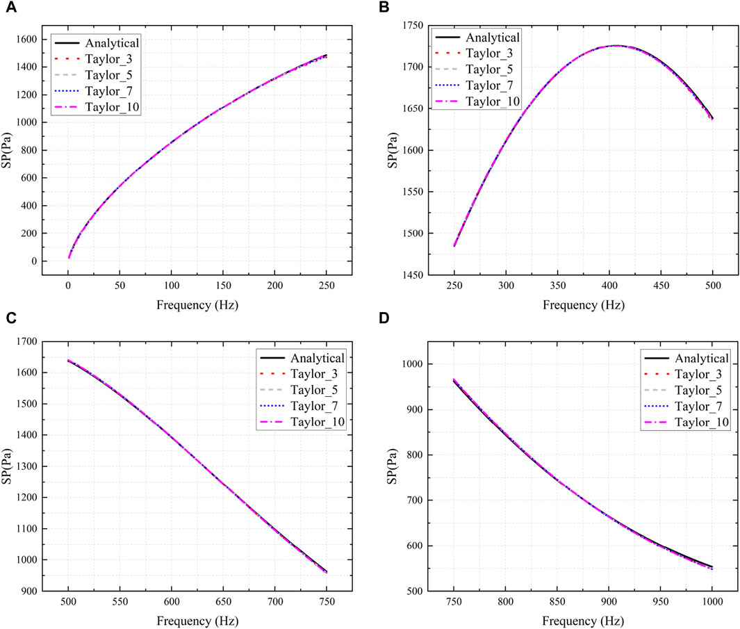
Figure 9. Sound pressure obtained using analytical solution and Taylor expansion methods. (A): 1–250 Hz, (B): 250–500 Hz, (C): 500–750 Hz, (D): 750–1000 Hz.

3.3 Sound barrier model

The acoustic analysis of a half-Y-shaped sound barrier (Figure 10) is carried out in this subsection. Figure 11 gives the real part, the imaginary part and the amplitude of the sound pressure at point (16, 2). It can be seen that the sound pressure exhibits variation among the different expansion terms, particularly at the extremities of the frequency range. Consequently, in this subsection, an adaptive band segmentation technique is employed to partition the frequency range of [1, 200] Hz into two sub-intervals. The sound pressure results of the two sub-intervals are shown in Figure 12. It can be seen that the results obtained demonstrate a remarkable consistency, irrespective of the number of expansion terms employed. This result just validates the effectiveness of the proposed adaptive band segmentation technique.

Figure 10

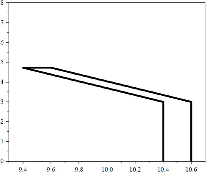
Figure 10. Half-Y-shaped sound barrier model.

Figure 11

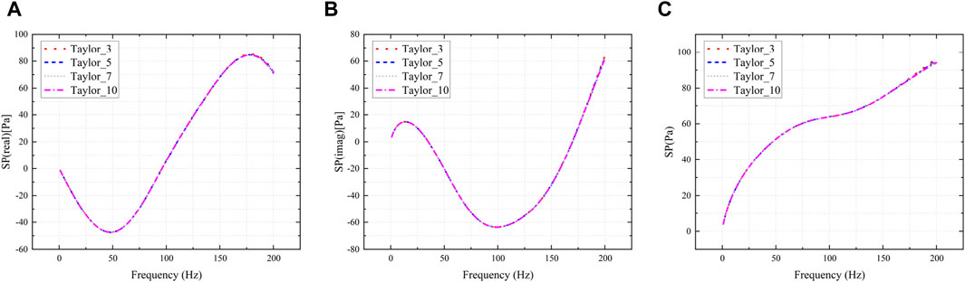
Figure 11. Sound pressure results at (16, 2) for the half-Y-shaped model. (A): the real part, (B): the imaginary part, (C): the amplitude.

Figure 12

Figure 12. Sound pressure at (16, 2). (A): 1–100 Hz, (B): 100–200 Hz.

Figure 13 compares the CPU time spent on the proposed method and CBEM for two different frequency settings. It can be seen that the proposed method exhibits a substantial decrease in CPU time when compared to CBEM. Although the CPU time escalates with an augmentation in the number of Taylor expansion terms, using Taylor expansion will still greatly reduce the CPU time used for wideband computation using the proposed method.

Figure 13

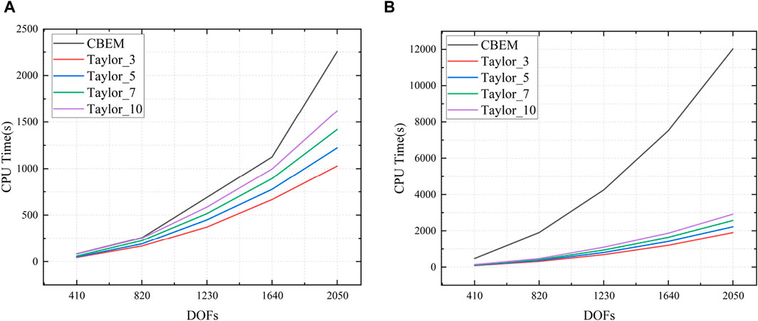
Figure 13. CPU time spent on numerical simulations using CBEM and Taylor expansion. (A): Frequency band (1, 100) Hz, step 1 Hz. (B): Frequency band (1, 100) Hz, step 0.1 Hz.

4 Conclusion

This paper focuses on the two-dimensional acoustic problems. The Burton-Miller method is used to solve the fictitious eigenfrequency problem. The Taylor expansion method is used to solve the problem of frequency dependence and low computational efficiency in wideband analysis, showing the time requirement advantage of the Taylor expansion over CBEM. The error in Taylor expansion-based analysis is reduced by narrowing the frequency bands. The validity of the adaptive frequency band segmentation technique is verified by comparing the sound pressure of each expansion term. The necessity of Taylor expansion is illustrated by comparing the CPU time. In practical engineering applications, the circular and airfoil arithmetic examples in this paper provide a reference for studying the noise problem of underwater vehicles. The Burton-Miller method and the Taylor expansion technique introduced in the paper are also able to be applied to other areas of acoustics.

Data availability statement

The original contributions presented in the study are included in the article/supplementary material, further inquiries can be directed to the corresponding author.

Author contributions

YY: Conceptualization, Funding acquisition, Investigation, Methodology, Project administration, Writing–original draft. GL: Conceptualization, Data curation, Visualization, Writing–original draft. SY: Validation, Writing–original draft. YX: Formal Analysis, Resources, Software, Supervision, Writing–review and editing.

Funding

The authors declare that financial support was received for the research, authorship, and/or publication of this article. Sponsored by the Henan Provincial Key R&D and Promotion Project under Grant No. 232102220033, the Henan Province science and technology research project under Grant No. 242102321031, the Youth Backbone Teacher Training Program of Henan Province under Grant No. 2019GGJS232, the Zhumadian 2023 Major Science and Technology Special Project under Grant No. ZMDSZDZX2023002, the Natural Science Foundation of Henan under Grant No. 222300420498, and the Postgraduate Education Reform and Quality Improvement Project of Henan Province under Grant No. YJS2023JD52.

Conflict of interest

The authors declare that the research was conducted in the absence of any commercial or financial relationships that could be construed as a potential conflict of interest.

Publisher’s note

All claims expressed in this article are solely those of the authors and do not necessarily represent those of their affiliated organizations, or those of the publisher, the editors and the reviewers. Any product that may be evaluated in this article, or claim that may be made by its manufacturer, is not guaranteed or endorsed by the publisher.

References

1. Lian H, Chen L, Lin X, Zhao W, Bordas SPA, Zhou M. Noise pollution reduction through a novel optimization procedure in passive control methods. Comput Model Eng Sci (2022) 131:1–18. doi:10.32604/cmes.2022.019705

CrossRef Full Text | Google Scholar

2. Ding C, Tamma K, Cui X, Ding Y, Li G, Bordas S. An nth high order perturbation-based stochastic isogeometric method and implementation for quantifying geometric uncertainty in shell structures. Adv Eng Softw (2020) 148:102866. doi:10.1016/j.advengsoft.2020.102866

CrossRef Full Text | Google Scholar

3. Marburg S. Developments in structural-acoustic optimization for passive noise control. Arch Comput Methods Eng (2002) 9:291–370. doi:10.1007/BF03041465

CrossRef Full Text | Google Scholar

4. Xu Y, Li H, Chen L, Zhao J, Zhang X. Monte Carlo based isogeometric stochastic finite element method for uncertainty quantization in vibration analysis of piezoelectric materials. Mathematics (2022) 10:1840. doi:10.3390/math10111840

CrossRef Full Text | Google Scholar

5. Chen L, Cheng R, Li S, Lian H, Zheng C, Bordas SP. A sample-efficient deep learning method for multivariate uncertainty qualification of acoustic–vibration interaction problems. Comput Methods Appl Mech Eng (2022) 393:114784. doi:10.1016/j.cma.2022.114784

CrossRef Full Text | Google Scholar

6. Zhao W, Chen L, Chen H, Marburg S. Topology optimization of exterior acoustic-structure interaction systems using the coupled fem-bem method. Int J Numer Methods Eng (2019) 119:404–31. doi:10.1002/nme.6055

CrossRef Full Text | Google Scholar

7. Zhao W, Chen L, Chen H, Marburg S. An effective approach for topological design to the acoustic-structure interaction systems with infinite acoustic domain. Struct Multidisciplinary Optimization (2020) 62:1253–73. doi:10.1007/s00158-020-02550-2

CrossRef Full Text | Google Scholar

8. Venås JV, Kvamsdal T. Isogeometric boundary element method for acoustic scattering by a submarine. Comput Methods Appl Mech Eng (2020) 359:112670. doi:10.1016/j.cma.2019.112670

CrossRef Full Text | Google Scholar

9. Shen X, Du C, Jiang S, Zhang P, Chen L. Multivariate uncertainty analysis of fracture problems through model order reduction accelerated sbfem. Appl Math Model (2024) 125:218–40. doi:10.1016/j.apm.2023.08.040

CrossRef Full Text | Google Scholar

10. Zhang G, Qu Y, Gao XL, Jin F. A transversely isotropic magneto-electro-elastic timoshenko beam model incorporating microstructure and foundation effects. Mech Mater (2020) 149:103412. doi:10.1016/j.mechmat.2020.103412

CrossRef Full Text | Google Scholar

11. Zhang GY, Guo ZW, Qu YL, Gao XL, Jin F. A new model for thermal buckling of an anisotropic elastic composite beam incorporating piezoelectric, flexoelectric and semiconducting effects. Acta Mechanica (2022) 233:1719–38. doi:10.1007/s00707-022-03186-7

CrossRef Full Text | Google Scholar

12. Shen X, Du C, Jiang S, Sun L, Chen L. Enhancing deep neural networks for multivariate uncertainty analysis of cracked structures by pod-rbf. Theor Appl Fracture Mech (2023) 125:103925. doi:10.1016/j.tafmec.2023.103925

CrossRef Full Text | Google Scholar

13. Coox L, Atak O, Vandepitte D, Desmet W. An isogeometric indirect boundary element method for solving acoustic problems in open-boundary domains. Comput Methods Appl Mech Eng (2017) 316:186–208. Special Issue on Isogeometric Analysis: Progress and Challenges. doi:10.1016/j.cma.2016.05.039

CrossRef Full Text | Google Scholar

14. Chen L, Lian H, Xu Y, Li S, Liu Z, Atroshchenko E, et al. Generalized isogeometric boundary element method for uncertainty analysis of time-harmonic wave propagation in infinite domains. Appl Math Model (2023) 114:360–78. doi:10.1016/j.apm.2022.09.030

CrossRef Full Text | Google Scholar

15. Zhang J, Zhou J, Wang S, Wang H, Lu F. Research on dynamic characteristics and radiation noise of a helicopter main reducer based on finite element and boundary element method. J Mech Sci Technol (2023) 37:4489–505. doi:10.1007/s12206-023-0807-9

CrossRef Full Text | Google Scholar

16. Zhang S, Yu B, Chen L. Non-iterative reconstruction of time-domain sound pressure and rapid prediction of large-scale sound field based on ig-drbem and pod-rbf. J Sound Vibration (2024) 573:118226. doi:10.1016/j.jsv.2023.118226

CrossRef Full Text | Google Scholar

17. Chen L, Chen H, Zheng C, Marburg S. Structural–acoustic sensitivity analysis of radiated sound power using a finite element/discontinuous fast multipole boundary element scheme. Int J Numer Methods Fluids (2016) 82:858–78. doi:10.1002/fld.4244

CrossRef Full Text | Google Scholar

18. Qu YL, Guo ZW, Zhang GY, Gao XL, Jin F. A new model for circular cylindrical Kirchhoff–love shells incorporating microstructure and flexoelectric effects. J Appl Mech (2022) 89:121010. doi:10.1115/1.4055658

CrossRef Full Text | Google Scholar

19. Liu Z, Bian PL, Qu Y, Huang W, Chen L, Chen J, et al. A galerkin approach for analysing coupling effects in the piezoelectric semiconducting beams. Eur J Mech - A/Solids (2024) 103:105145. doi:10.1016/j.euromechsol.2023.105145

CrossRef Full Text | Google Scholar

20. Marburg S The burton and miller method: unlocking another mystery of its coupling parameter. J Comput Acoust (2016) 24:1550016. doi:10.1142/s0218396x15500162

CrossRef Full Text | Google Scholar

21. Lian H, Kerfriden P, Bordas S. Shape optimization directly from cad: an isogeometric boundary element approach using t-splines. Comput Methods Appl Mech Eng (2017) 317:1–41. doi:10.1016/j.cma.2016.11.012

CrossRef Full Text | Google Scholar

22. Chen L, Marburg S, Zhao W, Liu C, Chen H. Implementation of isogeometric fast multipole boundary element methods for 2d half-space acoustic scattering problems with absorbing boundary condition. J Theor Comput Acoust (2018) 27:1850024. doi:10.1142/S259172851850024X

CrossRef Full Text | Google Scholar

23. Chen L, Lu C, Lian H, Liu Z, Zhao W, Li S, et al. Acoustic topology optimization of sound absorbing materials directly from subdivision surfaces with isogeometric boundary element methods. Comput Methods Appl Mech Eng (2020) 362:112806. doi:10.1016/j.cma.2019.112806

CrossRef Full Text | Google Scholar

24. Dölz J, Kurz S, Schöps S, Wolf F. Isogeometric boundary elements in electromagnetism: rigorous analysis, fast methods, and examples. SIAM J Scientific Comput (2019) 41:B983–B1010. doi:10.1137/18M1227251

CrossRef Full Text | Google Scholar

25. Sumbatyan M, Martynova T, Musatova N. Boundary element methods in diffraction of a point-source acoustic wave by a rigid infinite wedge. Eng Anal Boundary Elem (2021) 125:157–67. doi:10.1016/j.enganabound.2021.01.017

CrossRef Full Text | Google Scholar

26. Kurz S, Schöps S, Unger G, Wolf F. Solving maxwell’s eigenvalue problem via isogeometric boundary elements and a contour integral method. Math Methods Appl Sci (2021) 44:10790–803. doi:10.1002/mma.7447

CrossRef Full Text | Google Scholar

27. Cheng S, Wang F, Li PW, Qu W. Singular boundary method for 2d and 3d acoustic design sensitivity analysisimage 1. Comput Maths Appl (2022) 119:371–86. doi:10.1016/j.camwa.2022.06.009

CrossRef Full Text | Google Scholar

28. Chen L, Li K, Peng X, Lian H, Lin X, Fu Z. Isogeometric boundary element analysis for 2d transient heat conduction problem with radial integration method. CMES-Computer Model Eng Sci (2021) 126:125–46. doi:10.32604/cmes.2021.012821

CrossRef Full Text | Google Scholar

29. Chen L, Lian H, Liu Z, Gong Y, Zheng S. CJand Bordas. Bi-material topology optimization for fully coupled structural-acoustic systems with isogeometric fem–bem. Eng Anal Boundary Elem (2022) 135:182–95. doi:10.1016/j.enganabound.2021.11.005

CrossRef Full Text | Google Scholar

30. Chen L, Zhang Y, Lian H, Atroshchenko E, Ding C, Bordas S. Seamless integration of computer-aided geometric modeling and acoustic simulation: isogeometric boundary element methods based on catmull-clark subdivision surfaces. Adv Eng Softw (2020) 149:102879. doi:10.1016/j.advengsoft.2020.102879

CrossRef Full Text | Google Scholar

31. Chen L, Lian H, Dong H, Yu P, Jiang S, Bordas S. Broadband topology optimization of three-dimensional structural-acoustic interaction with reduced order isogeometric fem/bem. J Comput Phys (2024) 509:113051. doi:10.1016/j.jcp.2024.113051

CrossRef Full Text | Google Scholar

32. Chen L, Lian H, Liu Z, Chen H, Atroshchenko E, Bordas S. Structural shape optimization of three dimensional acoustic problems with isogeometric boundary element methods. Comput Methods Appl Mech Eng (2019) 355:926–51. doi:10.1016/j.cma.2019.06.012

CrossRef Full Text | Google Scholar

33. Qu Y, Jin F, Zhang G. Mechanically induced electric and magnetic fields in the bending and symmetric-shear deformations of a microstructure-dependent fg-mee composite beam. Compos Structures (2021) 278:114554. doi:10.1016/j.compstruct.2021.114554

CrossRef Full Text | Google Scholar

34. Cao G, Yu B, Chen L, Yao W. Isogeometric dual reciprocity bem for solving non-fourier transient heat transfer problems in fgms with uncertainty analysis. Int J Heat Mass Transfer (2023) 203:123783. doi:10.1016/j.ijheatmasstransfer.2022.123783

CrossRef Full Text | Google Scholar

35. Qu Y, Pan E, Zhu F, Jin F, Roy AK. Modeling thermoelectric effects in piezoelectric semiconductors: new fully coupled mechanisms for mechanically manipulated heat flux and refrigeration. Int J Eng Sci (2023) 182:103775. doi:10.1016/j.ijengsci.2022.103775

CrossRef Full Text | Google Scholar

36. Zheng CJ, Bi CX, Zhang C, Zhang YB, Chen HB. Fictitious eigenfrequencies in the bem for interior acoustic problems. Eng Anal Boundary Elem (2019) 104:170–82. doi:10.1016/j.enganabound.2019.03.042

CrossRef Full Text | Google Scholar

37. Toshimitsu R, Isakari H. A burton–miller-type boundary element method based on a hybrid integral representation and its application to cavity scattering. Eng Anal Boundary Elem (2024) 158:303–12. doi:10.1016/j.enganabound.2023.11.003

CrossRef Full Text | Google Scholar

38. Fu ZJ, Chen W, Gu Y. Burton–miller-type singular boundary method for acoustic radiation and scattering. J Sound Vibration (2014) 333:3776–93. doi:10.1016/j.jsv.2014.04.025

CrossRef Full Text | Google Scholar

39. Zheng CJ, Chen HB, Gao HF, Du L. Is the burton–miller formulation really free of fictitious eigenfrequencies? Eng Anal Boundary Elem (2015) 59:43–51. doi:10.1016/j.enganabound.2015.04.014

CrossRef Full Text | Google Scholar

40. Zhang J, Lin W, Shu X, Zhong Y. A dual interpolation boundary face method for exterior acoustic problems based on the burton–miller formulation. Eng Anal Boundary Elem (2020) 113:219–31. doi:10.1016/j.enganabound.2020.01.005

CrossRef Full Text | Google Scholar

41. Chen L, Marburg S, Chen H, Zhang H, Gao H. An adjoint operator approach for sensitivity analysis of radiated sound power in fully coupled structural-acoustic systems. J Comput Acoust (2017) 25:1750003. doi:10.1142/S0218396X17500035

CrossRef Full Text | Google Scholar

42. Wu Y, Dong C, Yang H. Isogeometric indirect boundary element method for solving the 3d acoustic problems. J Comput Appl Maths (2020) 363:273–99. doi:10.1016/j.cam.2019.06.013

CrossRef Full Text | Google Scholar

43. Chen L, Liu C, Zhao W, Liu L. An isogeometric approach of two dimensional acoustic design sensitivity analysis and topology optimization analysis for absorbing material distribution. Comput Methods Appl Mech Eng (2018) 336:507–32. doi:10.1016/j.cma.2018.03.025

CrossRef Full Text | Google Scholar

44. Liu X, Xu J. A low-frequency fast multipole boundary element method for acoustic problems in a subsonic uniform flow. Eng Anal Boundary Elem (2024) 162:102–16. doi:10.1016/j.enganabound.2024.01.026

CrossRef Full Text | Google Scholar

45. Liu B, Wang Q, Feng Y, Zhang ZS, Huang Q, Tian W, et al. The fast multipole method–accelerated line integration boundary element method for 3d heat conduction analysis with heat source. Eng Computations (2023) 40:1676–97. doi:10.1108/ec-03-2022-0157

CrossRef Full Text | Google Scholar

46. Li Y, Atak O, Desmet W. Novel and efficient implementation of multi-level fast multipole indirect bem for industrial helmholtz problems. Eng Anal Boundary Elem (2024) 159:150–63. doi:10.1016/j.enganabound.2023.11.027

CrossRef Full Text | Google Scholar

47. Zhang G, Gao X, Wang S, Hong J. Bandgap and its defect band analysis of flexoelectric effect in phononic crystal plates. Eur J Mech - A/Solids (2024) 104:105192. doi:10.1016/j.euromechsol.2023.105192

CrossRef Full Text | Google Scholar

48. Zhang G, Gao XL. A non-classical model for first-ordershear deformation circular cylindrical thin shells incorporating microstructure and surface energy effects. Maths Mech Sol (2021) 26:1294–319. doi:10.1177/1081286520978488

CrossRef Full Text | Google Scholar

49. Jin Q, Thompson DJ, Lurcock DE, Toward MG, Ntotsios E. A 2.5d finite element and boundary element model for the ground vibration from trains in tunnels and validation using measurement data. J Sound Vibration (2018) 422:373–89. doi:10.1016/j.jsv.2018.02.019

CrossRef Full Text | Google Scholar

50. Li Z, Gao Z, Liu Y. Enriched constant elements in the boundary element method for solving 2d acoustic problems at higher frequencies. Comput Model Eng Sci (2024) 138:2159–75. doi:10.32604/cmes.2023.030920

CrossRef Full Text | Google Scholar

51. Lei J, Shao C, Zhang C. Frequency-domain fundamental solutions and boundary element method for consistent couple stress elastodynamic problems. Int J Numer Methods Eng (2023) 124:4992–5019. doi:10.1002/nme.7335

CrossRef Full Text | Google Scholar

52. Li Y, Atak O, Jonckheere S, Desmet W. Accelerating boundary element methods in wideband frequency sweep analysis by matrix-free model order reduction. J Sound Vibration (2022) 541:117323. doi:10.1016/j.jsv.2022.117323

CrossRef Full Text | Google Scholar

53. Chen L, Lu C, Zhao W, Chen H, Zheng C. Subdivision surfaces—boundary element accelerated by fast multipole for the structural acoustic problem. J Theor Comput Acoust (2020) 28:2050011. doi:10.1142/s2591728520500115

CrossRef Full Text | Google Scholar

54. Wang Z, Zhao Z, Liu Z, Huang Q. A method for multi-frequency calculation of boundary integral equation in acoustics based on series expansion. Appl Acoust (2009) 70:459–68. doi:10.1016/j.apacoust.2008.05.005

CrossRef Full Text | Google Scholar

55. Ramzan M, Ahmad MO, Bashir MN, Asghar A, Shehzad SA. Development of numerical tools using boundary element method based on taylor series for nonlinear analysis. Mod Phys Lett B (2023) 37. doi:10.1142/s0217984923500501

CrossRef Full Text | Google Scholar

56. Han Z, Pan W, Cheng C, Hu Z, Niu Z. A semi-analytical treatment for nearly singular integrals arising in the isogeometric boundary element method-based solutions of 3d potential problems. Comput Methods Appl Mech Eng (2022) 398:115179. doi:10.1016/j.cma.2022.115179

CrossRef Full Text | Google Scholar

57. Riaz M, Hashmi MR, Pamucar D, Chu Y. Spherical linear diophantine fuzzy sets with modeling uncertainties in mcdm. Comput Model Eng Sci (2021) 126:1125–64. doi:10.32604/cmes.2021.013699

CrossRef Full Text | Google Scholar

58. Chen L, Lian H, Natarajan S, Zhao W, Chen X, Bordas S. Multi-frequency acoustic topology optimization of sound-absorption materials with isogeometric boundary element methods accelerated by frequency-decoupling and model order reduction techniques. Comput Methods Appl Mech Eng (2022) 395:114997. doi:10.1016/j.cma.2022.114997

CrossRef Full Text | Google Scholar

59. Chen L, Wang Z, Lian H, Ma Y, Meng Z, Li P, et al. Reduced order isogeometric boundary element methods for cad-integrated shape optimization in electromagnetic scattering. Comput Methods Appl Mech Eng (2024) 419:116654. doi:10.1016/j.cma.2023.116654

CrossRef Full Text | Google Scholar

60. Liu Y. On the bem for acoustic wave problems. Eng Anal Boundary Elem (2019) 107:53–62. doi:10.1016/j.enganabound.2019.07.002

CrossRef Full Text | Google Scholar

61. Zheng YT, Liu Y, Gao XW, Yang Y, Peng HF. Improved hole and tube elements in bem for elasticity problems. Eng Anal Boundary Elem (2024) 159:17–35. doi:10.1016/j.enganabound.2023.11.021

CrossRef Full Text | Google Scholar

62. Qu Y, Zhou Z, Chen L, Lian H, Li X, Hu Z, et al. Uncertainty quantification of vibro-acoustic coupling problems for robotic manta ray models based on deep learning. Ocean Eng (2024) 299:117388. doi:10.1016/j.oceaneng.2024.117388

CrossRef Full Text | Google Scholar

63. Dölz J, Harbrecht H, Kurz S, Schöps S, Wolf F. A fast isogeometric bem for the three dimensional laplace- and helmholtz problems. Comput Methods Appl Mech Eng (2018) 330:83–101. doi:10.1016/j.cma.2017.10.020

CrossRef Full Text | Google Scholar

64. Chen L, Zhao J, Lian H, Yu B, Atroshchenko E, Li P. A bem broadband topology optimization strategy based on taylor expansion and soar method-application to 2d acoustic scattering problems. Int J Numer Methods Eng (2023) 124:5151–82. doi:10.1002/nme.7345

CrossRef Full Text | Google Scholar