
95% of researchers rate our articles as excellent or good
Learn more about the work of our research integrity team to safeguard the quality of each article we publish.
Find out more
ORIGINAL RESEARCH article
Front. Phys. , 04 July 2024
Sec. Optics and Photonics
Volume 12 - 2024 | https://doi.org/10.3389/fphy.2024.1416064
This article is part of the Research Topic Advances in Infrared Lasers and Their Applications View all 9 articles
 Yan Wang1,2Jingting Liu3Chunyan Wang1,2
 Xinmin Fan1,2*
 Zhaohong Liu4Xiaodong Huang1,2Lujun Zhang1,2Sensen Li5*Yu Zhang6
Thermal action is a crucial process in laser processing. The classical Fourier heat conduction theory, which assumes an infinite speed of heat propagation, is commonly applied to describe steady-state and mild transient thermal processes. However, under the influence of ultra-short pulse lasers, such as those with picosecond and femtosecond durations, the heat propagation speed within the material is finite and deviates from Fourier’s law. This article addresses the unique characteristics of heat conduction in materials subjected to ultra-short pulse laser exposure by integrating Fourier’s law with the Gaussian distribution of the actual pulse laser output power density and the material’s optical absorption properties. It introduces a time variable to establish a time-dependent heat conduction equation. This equation is numerically analyzed using a difference algorithm. Based on this, simulation and experimental studies on the processing of dental hard tissues with a 1064 nm ps laser were conducted. The results show that the experimental processing depths were slightly larger than the simulation results, which may be due to damage to the dental hard tissues and the thermomechanical effects during processing. The results offer a technical reference for adjusting laser parameters in the ultra-short pulse laser processing technique.
Laser processing is a non-contact method utilizing thermal energy, requiring neither processing tools nor a special environment. It boasts high processing efficiency and exerts no mechanical force or thermal deformation on the workpiece [1, 2]. In practical laser processing applications, it is often necessary to modify laser irradiation conditions, specifically, the power density applied to the material. Achieving higher power density in-volves focusing the laser beam to concentrate energy within the focal area. Moreover, when operating in pulse mode, the laser releases energy instantaneously, and compressing the pulse width further increases power density [3]. The continual advancement of ultra-short pulse lasers, including picosecond and femtosecond lasers, has significantly enhanced laser power density and broadened their application in the laser processing field [4–7].
Upon irradiation onto a material, a portion of the light energy is absorbed and converted into heat energy. This heat then diffuses through the material via heat con-duction, inducing a specific temperature field distribution that alters the material’s properties within a certain range, ultimately resulting in the processed structure. The thermal action process is the most critical aspect of laser processing [8]. In engineering, the classical Fourier equation is commonly utilized to analyze and address heat conduction issues in materials under continuous laser exposure. Fourier’s law, predicated on the idealized assumption of infinitely fast heat propagation, neglects the effect of the heat transfer time variable [9, 10]. For lasers with nanosecond or longer pulse widths acting on materials, it is approximated that they conform to Fourier’s law. However, for ultra-short pulse lasers with pulse widths in the picosecond and femtosecond range, the material is heated super rapidly, the thermal action time is exceedingly short, the instantaneous heat flow density is incredibly high, and the heat exhibits fluctuations, i.e., finite speed propagation of wave heat flow, contradicting the assumptions of Fourier’s law [11–13]. The non-Fourier effect in heat conduction was first observed in supercooled nitrogen II, where heat conduction exhibited thermal wave behavior [14, 15], unexplainable by classical Fourier heat conduction theory. Subsequent experiments involving short-pulse laser heating of metal thin films revealed significant discrepancies be-tween the classical Fourier model predictions and measured results, with trends even appearing contradictory [16]. Additionally, the non-Fourier heat conduction effect has been observed in porous materials and biological tissues [17]. These findings indicate that the classical Fourier heat conduction model severely underestimates the instantaneous thermal elastic response level in unconventional heat conduction scenarios.
Non-Fourier heat conduction theory refines the classical model by introducing the concept of heat relaxation time or phase delay time based on Fourier’s law. Cattaneo and Vernottee proposed a non-Fourier constitutive equation based on the non-Fourier effect and local energy balance, respectively [18, 19]. Tzou highlighted the finite speed of heat propagation and the ensuing time delay, introducing the heat relaxation time τ, and developed models for both single-phase and double phase delay heat conduction [20, 21]. Wang and Tzou introduced a dual-phase lag heat conduction model to explore the non-Fourier heat transfer phenomena [22, 23]. In the realm of biological research, examining the non-Fourier mathematical models of heat transfer in biological tissues under laser exposure holds significant implications for laser thermotherapy [24, 25]. In essence, contemporary research emphasizes material specific characteristics, leading to the formulation of multiple non-Fourier equations for materials with varying properties under ultra-short pulse laser influence, thus challenging the development of a universal equation. Experimentally observing the non-Fourier effect in heat conduction proves exceedingly difficult, necessitating stringent experimental conditions, such as ultra-low temperatures, or highly sensitive instrument resolutions, like femtosecond-level laser heating processes. The experimental exploration of the non-Fourier heat conduction model remains limited due to these conditions, and the measurement of related model parameters is challenging, which hampers the broader application of non-Fourier heat conduction theory [26, 27].
In this paper, we aim to merge Fourier’s law with the Gaussian distribution of actual pulse laser output power density and the material’s optical absorption characteristics, intending to establish a time-dependent heat conduction model applicable under ultra-short pulse laser action. Building on this foundation, we theoretically simulated the processing depth of dental hard tissues with picosecond laser and conducted experimental verification. An analysis was performed on the discrepancies between the experimental results and theoretical simulation outcomes.
The MATLAB R2018a version was used for the simulation study of picosecond laser preparation of dental hard tissues.
A human molar, which was extracted for orthodontic reasons from the Department of Oral and Maxillofacial Surgery at Tianjin Medical University Dental Hospital and found to have intact dental hard tissues upon examination, was selected for the study. A micro-cutter was used to section the root, retaining only the crown for sample preparation. The crown was then cleaned in ultrasonic physiological saline for 20 min and soaked in saline for later use. The experimental laser (PICOPOWER-G1, Alphalas) was set to the following parameters: pulse width 20 ps, wavelength 1064 nm, repetition frequency 10 kHz, and average power 1 W, with a focus spot radius of 5 μm. The processing time was preset through CNC software, and the dimensions of the processed structure were measured using a confocal scanning microscope (Axio CSM700). After a laser action time of 0.02 s, the overall surface morphology of the processed area. The Scanning Electron Microscope (JSM-6700F) was opted to examine the microstructure of dental hard tissues.
For the entire laser processing process, the distribution of the temperature field in the material directly determines the change in material properties within a certain range, and ultimately determines the formation of the processing structure. Currently, most of the temperature field calculations in laser processing are based on the classic Fourier heat conduction model.
The mathematical expression of Fourier’s law is [36]:
In which, q is the heat flux density, k is the thermal conductivity, and grad T is the temperature gradient. q represents the heat flux per unit time on the unit area isothermal surface in the direction of decreasing temperature, and k characterizes the size of the thermal conductivity of the material, which is a positive scalar. Fourier’s law applies to steady and non-steady temperature fields in homogeneous and isotropic media. It reveals the relationship between the non-uniformity of temperature distribution and the heat conduction amount. However, Fourier’s law also has limitations. It cannot derive the connection between the temperature of a point and the temperature of its neighboring points, i.e., the intrinsic connection between the temperatures of neighboring points in a continuous temperature field, and it cannot derive the relationship between temperature and time changes. Fourier’s law can obtain the heat flux density corresponding to the determined temperature field in the object, but if the heat flux density is given, Fourier’s law cannot uniquely determine the temperature field. Therefore, the Fourier law is usually combined with the law of energy conservation to analyze and solve specific heat conduction problems.
From Eq. 1, we can see that as soon as the temperature distribution in an object becomes non-uniform due to a thermal disturbance somewhere, heat transfer will immediately occur. The speed of transfer is infinite. Even if infinitely far from the source of the thermal disturbance, it can be immediately affected by the disturbance source. This conclusion not only contradicts common physical sense but also cannot stand in a strictly theoretical sense. As known from the theory of statistical thermodynamics, an object usually shows certain inertia and damping characteristics for thermal disturbances, so the speed of thermal disturbance propagation in an object must be finite. For steady-state heat conduction problems, Fourier’s law can be accurately established. However, in a very short time, or under extremely high thermal load conditions, the impact of finite thermal propagation speed on heat conduction issues cannot be ignored [11].
For many heat conduction problems where the thermal action time is extremely short and the instantaneous heat flux density is extremely high, such as short pulse laser processing, when the pulse width of the laser is at the picosecond or femtosecond level, the heat propagation speed cannot be approximated as infinite. This leads to a sharp increase in temperature in a small area, and after the laser pulse action, the heat then diverges in all directions. To address this issue, a speed, or time variable, is introduced into the traditional Fourier equation to obtain a new heat conduction model. The introduction of this additional variable makes the temperature gradient in the medium related not only to the heat flow but also to the rate of change of heat flow with time. By applying the first-order Taylor series expansion to Eq. 1 with respect to time and ignoring the second and higher-order derivatives.
In this formula, q represents heat flux density, τ is the relaxation time, k stands for thermal conductivity, and grad T is the temperature gradient. The additional term introduced into this equation allows the propagation speed of the thermal disturbance to be finite.
Assuming that all thermal properties of the material in question do not vary with temperature, and that the laser beam used in processing is a fundamental mode Gaussian distribution, during the processing, the laser beam is perpendicular to the material surface, and convective and radiative heat transfer effects during the heating process are ignored. We establish the cylindrical coordinate system shown in Figure 1A, with selecting the center of the laser spot as the origin of the coordinates. As we assume that the laser beam is perpendicular to the material surface throughout the entire processing procedure, we can ignore the angular dimension, choosing the x-axis to be parallel to the material surface, and the z-axis to be perpendicular to the surface pointing towards the interior of the material.
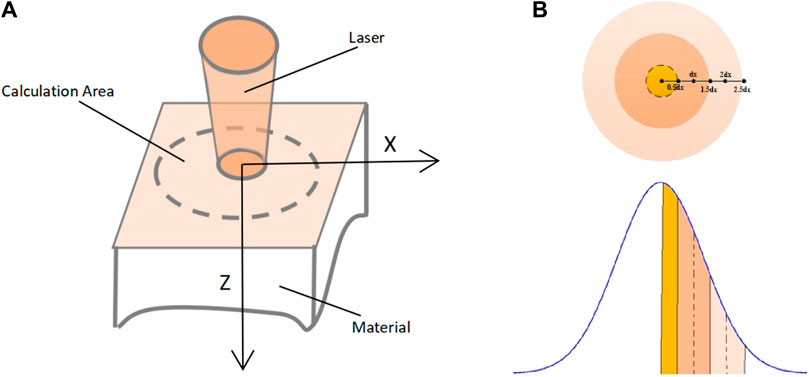
Figure 1. Schematic diagram of (A) laser processing; (B) lateral distribution of light intensity.
When building the model, we consider that the actual laser beam intensity has a certain spatial distribution. Generally, the laser propagates in the resonator in the basic transverse mode, and its spatial intensity distribution is Gaussian, approximately satisfying the Gaussian function. As known from laser principles, the field amplitude distribution of the basic transverse mode Gaussian beam is [28]:
Since the light intensity is directly proportional to the square of the amplitude, in Eq. 3, the intensity of the Gaussian beam can be represented as follows [29]:
In Eq. 4, is the light intensity at the light axis (r = 0), and is the beam radius.
For convenience in later numerical solutions, we use the concept of integration commonly used in advanced mathematics to derive the relationship between the central beam intensity with Gaussian distribution and the power density. Project the Gaussian beam onto the x-plane, and its light intensity lateral distribution is shown in Figure 1B. With point O as the center, it is divided into n circular rings with a radius of dx, the in-tensity of the ith circular ring is approximately taken as the intensity at the center point (i-1) dx (when 1 < i ≤ n), and the intensity of the first circular ring is taken as normalized intensity 1 (when i = 1).
Since light intensity is directly proportional to power density, the power density is also Gaussian distributed. Assuming the center power density is P0, then the light power Pi absorbed by each circular ring is related to the central power density P0 as follows:
Therefore, according to Eqs 5-8 the total absorbed light power is:
We know that the relationship between peak power P and average power is:
In Eq. 10, the fre is the repetition rate, and is the pulse width. The light energy irradiated on the material surface will not all be absorbed, and the absorbed light power can also be represented as:
In the formula, α is the absorption coefficient. Substitute Eq. 8 into Eq. 9 and combine it with Eq. 11 to get:
For lasers that are emitted in the TEM00 basic mode and have a Gaussian profile, the intensity and energy density values of the central beam need to be considered in the calculation. This central beam radius is defined as the aperture that can receive 93.61% of the incident power, at which point the beam radius is 0.6 ω. At this point, Eq. 12 can be rewritten as Eqs 13 and 14:
The standard unit of heat flux density is Wm-2, and the initial heat flux density caused by the light source is q0, as shown in Eq. 15. The piecewise function indicates that there is no heat flux distribution outside the range of the spot area.
For materials with a volume V, density ρ, and specific heat capacity C, the temperature rise caused by the absorbed energy ΔE can be expressed as:
Here, C refers to the specific heat capacity at constant pressure. All the thermal energy obtained by the material system is converted into an increase in its energy, so:
Substitute Eq. 17 into Eq. 16 to get:
Combining Eq. 18 with Eq. 2 gives:
The initial conditions and boundary conditions are:
In Eq. 20, the thermal relaxation time τ, thermal conductivity k, specific heat capacity C, and material density ρ are all determined by the material. T0 is the ambient temperature, and xw and zw are the boundaries. Sin, Sout, and the volume V are determined by the specific numerical calculation, and the initial heat flux density q0 is given by Eqs 14, 15.
In solving heat conduction problems, analytical and numerical methods emerge as the primary approaches. The analytical method, known for its exact solutions, offers clear physical concepts and logical reasoning throughout the solution process. Its foundation is relatively rigorous, yielding accurate and reliable solutions expressed in function form. This method effectively demonstrates how material properties, boundary conditions, and initial conditions influence temperature distribution. However, its application is limited to relatively simple heat conduction problems, and the precision of approximate analytical solutions may not match that achieved by numerical solutions [30].
Numerical methods, based on discrete mathematics, include the finite difference and finite element methods as the main techniques for addressing heat conduction issues. The finite element method provides greater convenience and flexibility in handling complex shapes compared to the finite difference method. However, for discrete representations of heat conduction problems, the finite difference formulation is simpler than that of the finite element method. Additionally, considering the development maturity and wide-spread application of these methods, the finite difference method holds a significant advantage [31–33].
In the cylindrical coordinate system established in Figure 1A, we assume that the origin is the first point of processing. Due to the symmetry of the cylinder, we can select 1/4 of the cylinder and discretize its cross section into a grid with step lengths of dx and dz. The intersection points between grid lines are called “nodes”, represented by (i, j), as shown in Figure 2A. Considering heat propagation as a unit cell, set the coordinates of the first cell in the upper left corner to (1,1), and the coordinates of the farthest point to (xN, zN). The coordinates of other cells are inferred in order.
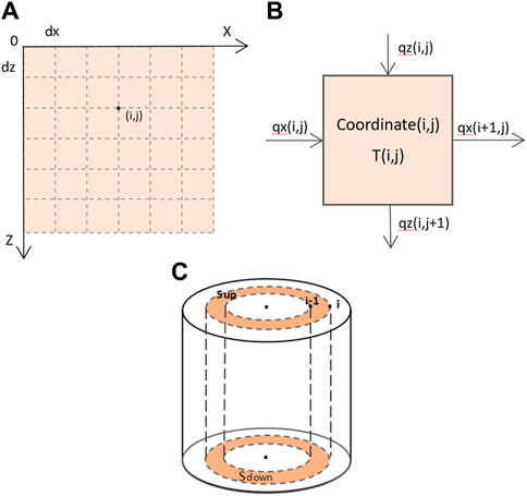
Figure 2. Schematic diagram of (A) differential grid division; (B) grid heat flow; (C) Heat conduction.
Eq. 15 can be discretized as Eq. 21:
Substituting the difference equation for the differential equation of Eq. 2, Eq. 21 can be expressed as
After simplifying the above Eqs 22 and 23, the following formula can be obtained as Eqs 24 and 25:
In the context of a discretized grid with coordinates (i, j), we define the temperature of a given grid cell as T (i, j). T (i, j) represents the temperature of the entire cell. Given the physical meaning of heat flux, the discretized heat flux is only meaningful at the interface between two adjacent cells. We define the heat flux flowing into the left boundary in the X-direction, x (i, j), combined with the heat flux flowing into the upper boundary in the Z-direction, z (i, j), as qin. This is the total heat flux in the X-direction at the grid point defined by the grid cell.
Similarly, in Figure 2B, the sum of the heat flux flowing out of the right boundary in the X-direction, qx (i+1, j), and the heat flux flowing out of the lower boundary in the Z-direction, qz (i, j+1), is defined as qout. Here, qx (i+1, j) represents the heat flux in the X-direction flowing into the next cell, and similarly, qz (i, j+1) represents the heat flux in the Z-direction flowing into the next cell.
The definition of the areas of each boundary of a grid cell is shown in Figure 2C. The area of the top surface is that of an annulus with an outer radius of idx and an inner ra-dius of (i-1)dx; the area of the bottom surface is the same as the top surface. The area of the left boundary is defined as the lateral surface area of a right circular cylinder with a base radius of (i-1)dx, and the area of the right boundary is defined as the lateral surface area of a right circular cylinder with a base radius of idx.
The formula for the area of each boundary surface is as follows:
For each cell, the input power is the sum of the upper boundary input power and the left boundary input power, and its expression is
The output power is the sum of the output power of the lower boundary and the output power of the right boundary, and its expression is
Substituting Eqs 26, 27 into Eq. 17, the temperature change after dt time can be obtained as
The initial temperature of all grid cells is T0. Based on the heat flow in and out of the grid cells, Told can be gradually updated to Tnew. According to the above equation, the temperature T (i,j) of the grid cell at coordinates (i,j) after time dt can be derived. After the temperatures of all grid cells have been calculated, all qz and qx can be updated based on Eqs 28, 29.
According to Eq. 30, the analysis of boundary conditions is as follows:
When j = 1, it is the upper surface where the part irradiated by the laser has qz (i,1) given by the laser parameters, and the rest is 0. qz (i,1) is determined by the input and does not need to be updated. In addition, considering that T (i, j-1) is meaningless when j = 1 (it is agreed that the coordinates start from (1,1), skipping qz (i,1) and starting the update from j = 2 avoids this situation.
When i = 1, the area of the left surface of the cell is 0, so whether or not qx (1, j) is up-dated does not affect the correctness of the results. Thus, although qx (1, j) needs to be updated, starting the update from j = 2 does not affect the calculation results.
When j = zN, this corresponds to reaching the edge of the material. Assume the ma-terial edge interfaces with a constant-temperature environment. Now, the cell coordinates are (i, zN), and the heat flux at the lower boundary of the cell is qz (i, zN+1). Initially, qz (i, zN+1) is 0, but the update of heat flux necessitates Δqz (x, zN+1). Because calculating Δqz (x, zN+1) requires the temperature T (i, zN+1), which is undefined, we maintain uniformity by appending a constant temperature T (i, N+1) = T0 at the end of the temperature T array, substituting the environment’s temperature T0 for T (i, zN+1). This lets us continue using the original formula to calculate Δqz (i, zN+1), ensuring the program’s consistency. Moreover, T (i, zN+1) is not updated in the program, which is aligned with the constant temperature of the interfacing environment. Similarly, the processing method of i = xN is consistent with that of j = zN, so for a material with xN*zN cells, the temperature coordi-nates need to be increased to (xN+1, zN+1), and the outermost layer represents the temperature of the external environment.
Lasers have been widely used in dental surgery, where the thermal effects generated during laser ablation can not only remove tooth material but may also cause damage to the soft tissues of the dental pulp. Therefore, simulating the internal temperature field of teeth during the laser preparation process and comparing it with experimental results can explore the related photothermal action mechanisms and improve the design and optimization of clinical treatment strategies. Based on Eq. 19 and the aforementioned theoretical results, we utilize MATLAB for the simulation study of picosecond laser preparation of dental hard tissues and conducts a comparative analysis with experimental results.
When the laser irradiates the tooth surface, the following three processes primarily occur: 1) The water and inorganic substances in the dental hard tissues absorb the laser energy and heat up. 2) The water and inorganic substances within the tooth evaporate. 3) The organic substances in the tooth hard tissues chemically decompose, along with the decomposition of hydroxyapatite. Hydroxyapatite, which makes up more than 70% of dental hard tissues, has a melting point and boiling point of 1100°C and 1500°C, respectively [34]. Hard tissue ablation is generally applied in cases where the depth of caries has reached the dentin, hence the selection of dentin’s parameters as the material parameters for the simulation. The thermal conductivity of dentin is found to be 0.88 (W/(m·K)) from literature [35]. Dentin’s thermal conductivity is already in the range of insulators, and its thermal relaxation time is chosen at the insulator scale of 1 × 10⁻¹³ s [36]. At a wavelength of 1064 nm, the optical absorption ratio is about 0.58, and the specific heat capacity is 1.17 (J/(g·K)) [35]. The laser parameters for theoretical simulation are pulse width 20 ps, wavelength 1064 nm, repetition frequency 10 kHz, and average power 1 W.
Figure 3 illustrates the temperature field distribution within dental hard tissues under the influence of a single pulse, where the white line marked areas denote the corresponding damage range. It is observed that the picosecond laser’s single pulse thermal damage range is within the micron scale, aligning with the characteristic of dental hard tissues as poor thermal conductors. The simulation results also reveal that the distance between the damage range and the structure formation range decreases over time. The laser used in the simulation operates at a frequency of 10 kHz, corresponding to a pulse interval of 10−4s, while the duration of pulse action is only 2 × 10⁻¹³ s. Compared to the pulse action time, the pulse interval is sufficiently long to allow for temperature dissipation within this period. Based on this, it is considered safe to use picosecond laser ablation on dental hard tissues when the ablation area is at a micrometer level away from the dental pulp cavity. While this may cause pain, it will not damage the dental pulp. Ultimately, the calculations indicate that drilling to a depth of 200 μm requires 544 pulses, with a single pulse achieving a processing depth of 0.368 μm.
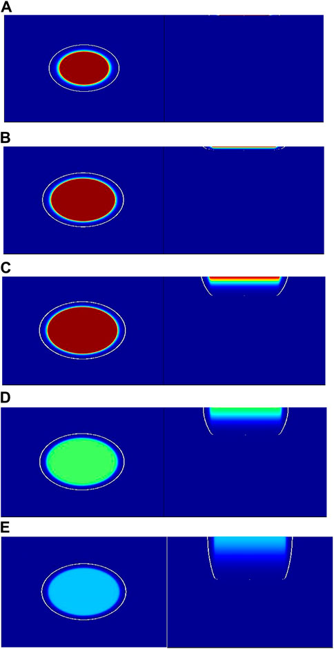
Figure 3. Horizontal temperature field distribution and vertical temperature field distribution within the tooth. (A) 1e−14 s; (B) 1e−13 s; (C) 2e−12 s; (D) 4e−12 s; (E) 1e−11 s.
The final step involves a comparison with experimental results. As shown in Figure 4A, observation of the surface morphology postprocessing reveals a slight darkening around the processed hole, indicating the presence of thermal effects within the material. Figure 4B displays the specific measurement results of the processed structure dimensions. A total of 200 pulses achieved a hole depth of 90.699 μm, with a single pulse processing depth of 0.453 μm.
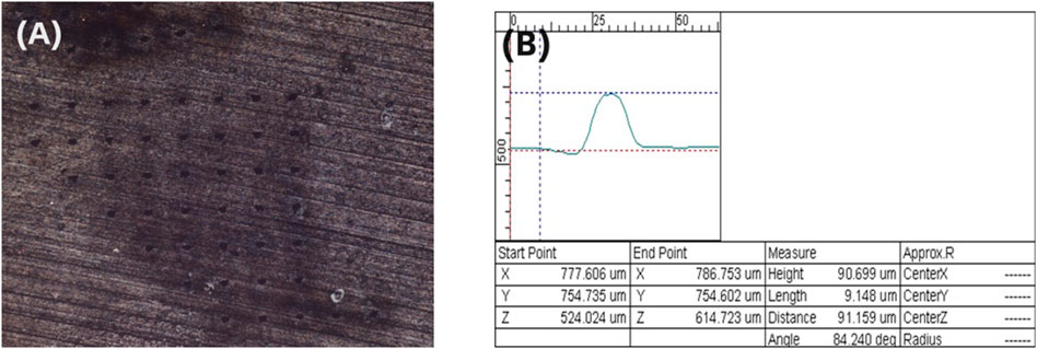
Figure 4. (A) Overall surface morphology post-processing observed under a confocal microscope; (B) Measurement of processed structure dimensions under a confocal microscope.
Comparative analysis reveals that the theoretical calculation of single pulse processing depth is smaller. In analyzing factors that might influence the discrepancies, we consider that the unique structure of dental hard tissues could affect the experimental outcomes. Given this, we opted to examine the microstructure of dental hard tissues using a Scanning Electron Microscope with the overall tooth cross-section displayed in Figure 5A, where the outer layer is the enamel, and the inner layer is the dentin (the honeycomb structure is conductive gel). Figures 5B, C illustrate that both the surface of the dentin and enamel are uneven, with numerous pits and fissures present in the dentin. From this, we hypothesize that the porous nature of dental hard tissues is one of the crucial reasons for the larger experimental values. Additionally, we analyze that the laser pulses might carry kinetic energy upon reaching the material surface, and the final structure formation could be the cumulative effect of laser kinetic and thermal energy, with the thermomechanical action causing an increase in the processing depth observed experimentally. Moreover, no inert assist gas was used in the experiments, meaning oxygen in the air could react with the material, releasing thermal energy as an additional heat source apart from the laser, thus enlarging the thermal affected zone. To align simulation results more closely with actual experimental outcomes, extensive experimentation is necessary to derive patterns from experimental data, refine the simulation model, and introduce correction factors.
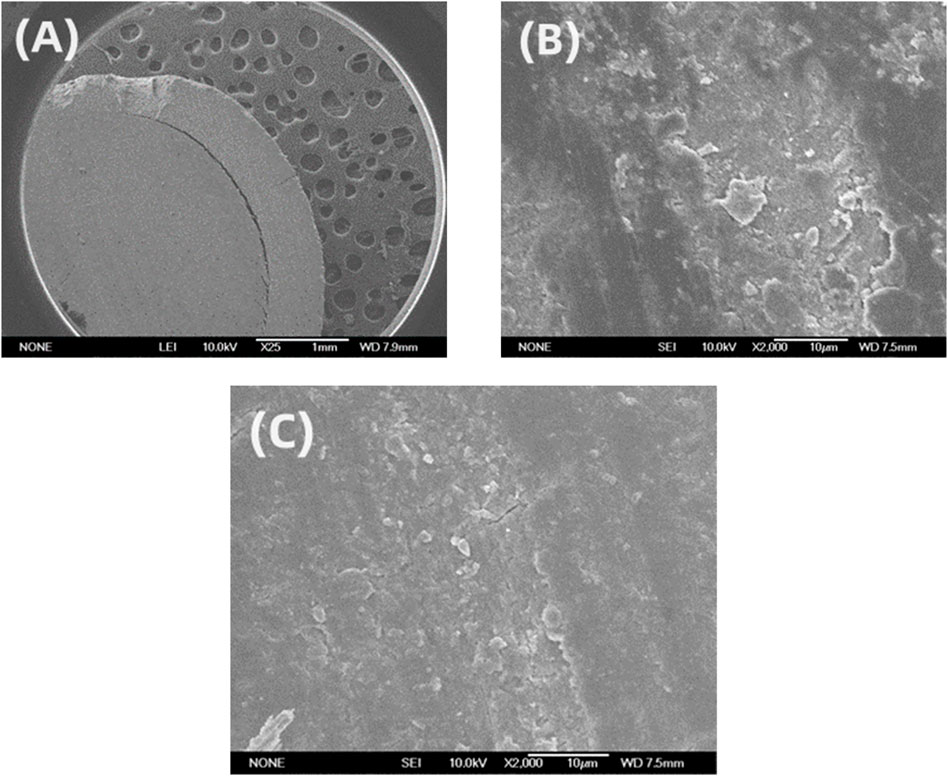
Figure 5. (A) Overall tooth cross-section observed at ×25 magnification under a SEM; (B) Enamel surface observed at 2000 × magnification under a SEM; (C) Dentin surface observed at 2000 × magnification under a SEM.
For heat conduction scenarios characterized by extremely brief heat exposure durations and exceedingly high instantaneous heat flux densities, such as those encountered in ultra-short pulse laser processing with pulse widths on the order of picoseconds or femtoseconds, the assumption of infinite heat propagation speed becomes untenable. Under these conditions, predictions made by the classical Fourier heat conduction model significantly diverge from observed outcomes. It is, therefore, imperative to formulate a non-Fourier heat conduction equation that accurately encapsulates the heat conduction behaviors of materials subjected to ultra-short pulse lasers. This paper introduces a time-dependent heat conduction equation tailored for ultra-short pulses, including those in the picosecond and femtosecond ranges. Employing the finite difference method, this equation is numerically solved to delineate the temperature field distribution within a material following exposure to a single pulse. Based on the theoretical research outcomes, simulations for processing dental hard tissues with a 1064 nm ps laser were conducted, achieving a single pulse processing depth of 0.368 µm. Experimental verification yielded a single pulse processing depth of 0.453 µm. We analyze that the porous physiological structure of teeth, along with the model’s failure to consider the thermomechanical effects during the ultra-fast laser processing, results in theoretical simulation outcomes being lower than the experimental data. In subsequent work, based on extensive experimentation, the heat conduction equation will be further revised, and appropriate correction factors will be introduced through experimental and theoretical simulation.
The original contributions presented in the study are included in the article/supplementary material, further inquiries can be directed to the corresponding authors.
YW: Conceptualization, Data curation, Formal Analysis, Investigation, Methodology, Project administration, Writing–original draft. JL: Data curation, Investigation, Supervision, Writing–original draft. CW: Writing–review and editing. XF: Data curation, Methodology, Writing–review and editing. ZL: Resources, Supervision, Writing–review and editing. XH: Funding acquisition, Supervision, Writing–review and editing. LZ: Resources, Supervision, Writing–review and editing. SL: Conceptualization, Data curation, Writing–review and editing. YZ: Funding acquisition, Writing–review and editing.
The author(s) declare that financial support was received for the research, authorship, and/or publication of this article. This work was funded by the National Key Research and Development Program of China (501100012166) and the Open Project Program of Shanxi Key Laboratory of Advanced Semiconductor Optoelectronic Devices and Integrated Systems (2023SZKF22).
The authors declare that the research was conducted in the absence of any commercial or financial relationships that could be construed as a potential conflict of interest.
All claims expressed in this article are solely those of the authors and do not necessarily represent those of their affiliated organizations, or those of the publisher, the editors and the reviewers. Any product that may be evaluated in this article, or claim that may be made by its manufacturer, is not guaranteed or endorsed by the publisher.
1. Son Y, Yeo J, Moon H, Lim TW, Hong S, Nam KH, et al. Nanoscale electronics: digital fabrication by direct femtosecond laser processing of metal nanoparticles. Adv Mater (2011) 23(28):3176–81. doi:10.1002/adma.201100717
2. Wu J, Liu X, Qiao H, Zhao Y, Hu X, Yang Y, et al. Using an artificial neural network to predict the residual stress induced by laser shock processing. Appl Opt (2021) 60(11):3114. doi:10.1364/ao.421431
3. Li Y, Shi Y, Zhang Z, Xing D. Nonlinearly enhanced photoacoustic microscopy by picosecond-laser-pumped excited state absorption of phthalocyanine nanoprobes. Appl Phys Lett (2021) 118(19):193701. doi:10.1063/5.0050767
4. Bai S, Serien D, Hu A, Sugioka K. 3D microfluidic surface-enhanced Raman spectroscopy (SERS) chips fabricated by all-femtosecond-laser-processing for real-time sensing of toxic substances. Adv Funct Mater (2018) 28:1706262. doi:10.1002/adfm.201706262
5. Guo H, Yan J, Jiang L, Deng S, Lin X, Qu L. Femtosecond laser bessel beam fabrication of a supercapacitor with a nanoscale electrode gap for high specific volumetric capacitance. ACS Appl Mater Inter (2022) 14(34):39220–9. doi:10.1021/acsami.2c10037
6. Santos SNC, Romero ALS, Menezes BC, Garcia R, Almeida J, Hernandes A, et al. Femtosecond-laser fabrication of magneto-optical waveguides in terbium doped CaLiBO glass. Opt Mater (2022) 126:112197. doi:10.1016/j.optmat.2022.112197
7. Liao K, Wang W, Mei X, Liu B. High quality full ablation cutting and stealth dicing of silica glass using picosecond laser Bessel beam with burst mode. CERAMICS INTERNATIONAL (2022) 48(7):9805–16. doi:10.1016/j.ceramint.2021.12.182
8. Prusa JM, Venkitachalam G, Molian PA. Estimation of heat conduction losses in laser cutting. Int J Machine Tools Manufacture (1999) 39(3):431–58. doi:10.1016/s0890-6955(98)00041-8
9. Nika G. A gradient system for a higher-gradient generalization of Fourier's law of heat conduction. Mod Phys Lett B (2023) 37(11). doi:10.1142/s0217984923500112
10. Zhang XY, Li XF. Thermal performance of a convective functionally graded fin using fractional non-fourier heat conduction. J Thermophys Heat Transfer (2021)(1) 1–10.
11. Mao YD, Xu MT. Non-Fourier heat conduction in a thin gold film heated by an ultra-fast-laser. ence China Technol ences (2015) 58(4):638–49. doi:10.1007/s11431-015-5767-6
12. Poshti AGT, Khosravirad A, Ayani MB. Analyses of non-Fourier heat conduction in 1-D spherical biological tissue based on dual-phase-lag bio-heat model using the conservation element/solution element (CE/SE) method: a numerical study. Int Commun Heat Mass Transfer: A Rapid Commun J (2022) 132:105881. doi:10.1016/j.icheatmasstransfer.2022.105881
13. Rashidi-Huyeh M, Volz S, Palpant B. Non-Fourier heat transport in metal-dielectric core-shell nanoparticles under ultrafast laser pulse excitation. Phys Rev B (2008) 78(12):125408. doi:10.1103/physrevb.78.125408
16. Qiu TQ, Juhasz T. Femtosecond laser heating of muti-layer metals. Int J Heat Mass Transfer (1994) 37(17):2799–808.
17. Han-Taw C, Jae-Yuh L. Numerical analysis for hyperbolic heat conduction. Int J Heat Mass Transfer (1993) 36(11):2891–8. doi:10.1016/0017-9310(93)90108-i
18. Cattaneo C. A form of heat conduction equation which eliminates the paradox of instantaneous propagation. Compte Rendus (1958) 247(4):431–3.
19. Vernotte P. Paradoxes in the continuous theory of the heat equation. Compte Rendus (1958) 246(3):154–5.
20. Tzou DY. Thermal shock phenomena under high-rate response in solids. Annu Rev Heat Transfer (1992) 4:111–85. doi:10.1615/annualrevheattransfer.v4.50
21. Tzou DY. A unified field approach for heat conduction from macro-to micro-scales. ASME J Heat Transfer (1995) 117:8–16. doi:10.1115/1.2822329
22. Wang BL, Han JC. Thermal conduction in bi-layer materials with an interfacial inclusions. Phil Mag Lett (2011) 90:241–9.
23. Tzou DY. The generalized lagging response in small-scale and high-rate heating. Int J Heat Mass Transfer (1995) 38:3231–40. doi:10.1016/0017-9310(95)00052-b
24. Hamed ZP, Hassan M, Amir M. Analysis of the dual phase lag bio-heat transfer equation with constant and time-dependent heat flux conditions on skin surface. Therm Sci (2016) 20(5):1457–72.
25. Biswas P, Singh S, Bindra H. A closed form solution of dual phase lag heat conduction problem with time periodic boundary conditions. J Heat Transfer (2019) 141(3):031302.1–031302.12. doi:10.1115/1.4042491
26. Guo SL, Wang B, Li J. Surface thermal shock fracture and thermal crack growth behavior of thin plates based on dual-phase-lag heat conduction. THEORETICAL APPLIED FRACTURE MECHANICS (2018) 96:105–13. doi:10.1016/j.tafmec.2018.04.007
27. Guo SL, Wang BL. Thermal shock cracking behavior of a cylinder specimen with an internal penny-shaped crack based on non-fourier heat conduction. Int J Thermophys (2016) 37(2):17–23. doi:10.1007/s10765-015-2029-6
29. Xu YS, Guo ZY. Heat wave phenomena in IC chips. Int J Heat Mass Transfer (1995) 38(15):2919–22. doi:10.1016/0017-9310(95)00007-v
30. Miller ST, Haber RB. A spacetime discontinuous galerkin method for hyperbolic heat conduction. Comp Methods Appl Mech Eng (2008) 198(2):194–209. doi:10.1016/j.cma.2008.07.016
31. Glass DE, Qzisik MN, Brian V. Hyperbolic heat conduction with surface radiation. Int J Heat Mass Transfer (1985) 28(7):1823–30.
32. Wiggert DC. Analysis of early-time transient heat conduction by method of characteristics. Transaction Asme, J Heat Transfer (1997) 114:35–40. doi:10.1115/1.3450651
33. Hu W, Fu Z, Tang Z, Gu Y. A meshless collocation method for solving the inverse Cauchy problem associated with the variable-order fractional heat conduction model under functionally graded materials. Eng Anal boundary Elem (2022) 140:132–44. doi:10.1016/j.enganabound.2022.04.007
34. Dostálová T, Jelínková H, Nemec M, Koranda P, Miyagi M, Iwai K, et al. Er:YAG laser micro-preparation of hard dental tissue. BMJ (2007) 317(7156):465–8. doi:10.1117/12.698148
35. Little PAG, Wood DJ, Bubb NL, Maskill SA, Mair LH, Youngson CC. Thermal conductivity through various restorative lining materials. J Dent (2005) 33:585–91. doi:10.1016/j.jdent.2004.12.005
Keywords: laser processing, ultra-short pulse, non-fourier heat conduction, numerical analysis, temperature field
Citation: Wang Y, Liu J, Wang C, Fan X, Liu Z, Huang X, Zhang L, Li S and Zhang Y (2024) Numerical analysis and experimental verification of time-dependent heat conduction under the action of ultra-short pulse laser. Front. Phys. 12:1416064. doi: 10.3389/fphy.2024.1416064
Received: 11 April 2024; Accepted: 17 May 2024;
Published: 04 July 2024.
Edited by:
Quan Sheng, Tianjin University, ChinaReviewed by:
Pibin Bing, North China University of Water Conservancy and Electric Power, ChinaCopyright © 2024 Wang, Liu, Wang, Fan, Liu, Huang, Zhang, Li and Zhang. This is an open-access article distributed under the terms of the Creative Commons Attribution License (CC BY). The use, distribution or reproduction in other forums is permitted, provided the original author(s) and the copyright owner(s) are credited and that the original publication in this journal is cited, in accordance with accepted academic practice. No use, distribution or reproduction is permitted which does not comply with these terms.
*Correspondence: Xinmin Fan, eGlubWluZmFuQHdmdS5lZHUuY24=; Sensen Li, bGlzZW5zZW5AY2V0Yy5jb20uY24=
Disclaimer: All claims expressed in this article are solely those of the authors and do not necessarily represent those of their affiliated organizations, or those of the publisher, the editors and the reviewers. Any product that may be evaluated in this article or claim that may be made by its manufacturer is not guaranteed or endorsed by the publisher.
Research integrity at Frontiers
Learn more about the work of our research integrity team to safeguard the quality of each article we publish.