Air quality prediction based on quantum activation function optimized hybrid quantum classical neural network

Accurate prediction of air quality index is a challenging task, in order to solve the gradient problem of traditional neural network methods in the time series prediction process as well as to improve the prediction accuracy, the study proposes a hybrid quantum neural network prediction model based on quantum activation function. The model utilizes a quantum classical convolutional neural network to tap into spatial correlations between different time periods and combines it with a quantum activation function so as to better avoid the gradient problem and solve the death RELU problem for better spatial feature extraction, and then uses the long short term memory neural network to capture the observations at different times. Experiments were conducted on different air quality datasets using the model, which proved that the proposed quantum activation function optimized hybrid quantum neural network algorithm showed more remarkable advantages in prediction accuracy than other model algorithms.

1 Introduction

The Air Quality Index (AQI) is widely used to assess air quality, and its results can fully reflect the actual air quality conditions [1–3]. Air quality problems [4] have a certain impact on various industries, with a greater impact on healthcare [5], tourism [6], and economy [7]. Currently, two main types of methods are used for air quality prediction: linear regression models and neural network models. Among these methods, support vector machine (SVM) [8] and neural network [9] based models are particularly typical. Support vector machines have been widely used as an algorithm for a variety of forecasting tasks including time series data. For example, support vector regression-based prediction models consider weather factors [10] and support vector machine-based weather prediction methods [11]. Traditional neural network models, such as for the complex problem of air quality prediction, Chen and other researchers proposed an innovative prediction model that uses an architecture that combines a dual LSTM (Long Short-Term Memory Network). This architecture aims to improve the accuracy of the prediction results and the robustness of the model [12]. 2019 Zahra Karevan et al. developed a data-driven weather forecasting model based on LSTM to apply it in the field of weather forecasting. In addition, an improved variant of LSTM called transduction LSTM (T-LSTM) was proposed, which focuses on utilizing local information to improve the accuracy of time series prediction. The results of the study show that T-LSTM exhibits superior performance to conventional methods in performing forecasting tasks [13]. Zhang et al. proposed a Convolutional Neural Network-Long Short-Term Memory (CNN-LSTM) model aimed at improving air quality prediction accuracy [14]. However, there are still many problems with current AI techniques when solving time series prediction problems. The analysis speed of classical computers may not be able to keep up with the real-world challenges of changing weather conditions [15]. In addition, the gradient problem may still be faced in the case of very long time series data. Gradients in long time series are difficult to propagate through the network, which leads to the model’s inability to learn the long-term time dependence. As quantum technology continues to advance, machine learning algorithms [16] and advances in the field of quantum computing ([17]; [18]) offer potential possibilities for creating accurate air quality prediction models. Common quantum architectures proposed so far include quantum BP neural networks based on generalized quantum gate evolution [19], quantum neural networks based on extreme learning machines [20], quantum multilayer perceptron neural networks [21], quantum neural networks (QNN) [22], quantum convolutional neural networks (QCNN), and quantum long and short-term memory networks (QLSTM) [23]. Quantum machine learning has become a current research hotspot in the field of neural networks. Mitarai et al. proposed a hybrid classical-quantum QML algorithm using Variational Quantum Circuits (VQCs) [24], where VQCs can learn a given task by tuning the parameters implemented on them. Inspired by quantum computing, Chen Gong et al. proposed a quantum particle swarm optimization algorithm based on a diversity migration strategy by combining the traditional migration strategy with the average Hamming distance to increase the population diversity, and the results show that the proposed algorithm outperforms other typical optimization algorithms and has stable convergence [25]. Li-Hua Gong et al. proposed a quantum K-nearest neighbor algorithm based on the divide-and-conquer strategy, which utilizes quantum circuits to calculate the fidelity between the test samples and each feature vector of the training dataset, and demonstrates higher classification efficiency in high-dimensional data processing, and the proposed classification method has higher classification accuracy and shorter computation time compared with typical quantum K-nearest neighbor algorithms [26]. Nan-Run Zhou et al. designed an image generation scheme based on quantum generative adversarial network to convert the multimodal distribution of the image into a single peak distribution by remapping method and optimized the structure of the quantum generator to reduce the required parameters, which led to the successful generation of MNIST image and Fashion-MNIST image [27]. In 2019, Quantum Convolutional Neural Network (QCNN) proposed by Cong et al. extends the main features of CNN to quantum systems for dealing with quantum physics problems in Hilbert space, avoiding the exponential growth of data volume caused by transferring quantum data to classical computing environments [28]. Herrmann et al. proposed a novel quantum convolutional neural network (QCNN) specifically designed for phase classification and optimization of quantum error correcting codes. This QCNN is structurally similar to conventional CNNs and has the same network architecture [29]. Li-Hua Gong et al. designed a quantum convolutional neural network (QCNN) based on variational quantum circuits, and developed a tree-structured hybrid magnitude coding method by combining the advantages of angle coding and magnitude coding, and the experiments showed that the QCNN achieves faster convergence speed and higher image classification accuracy compared to classical convolutional neural networks [30]. In 2022 Eric Paquet et al. proposed a new hybrid deep quantum neural network for time series prediction, the QuantumLeap system, and the experimental results clearly demonstrated the accuracy and efficiency of the system in regression and extrapolation mechanisms [31]. Researchers such as Andrea Ceschini have proposed an innovative architecture that combines stacked long and short-term memory layers with variational quantum layers. This method achieves a significant improvement in prediction error, demonstrating the ability to approximate stochastic fluctuations more accurately. In addition, the quantum variational approach has demonstrated its overall effectiveness in performing prediction tasks [32]. Hong et al. combined quantum-inspired neural networks for time series prediction by cascading parallel convolutional neural networks with both long and short-term memory and quantum-inspired neural networks in order to realize an innovative neural network technique. The results show that the proposed method outperforms other methods in time series forecasting [33].

An innovative hybrid model is proposed to face the many challenges in air quality prediction research nowadays, such as poor prediction accuracy and computational efficiency. The contribution of this paper is as follows.

i. Based on the concept of variational quantum circuits [34], a quantum hybrid neural network prediction structure (HQCNN-LSTM) is designed. The quantum classical neural network (HQCNN) is used to extract the features of the time series data to form the input feature vector, which consists of a quantum convolutional layer and a classical convolutional layer. The quantum convolutional layer has three parts: coding [35], parameterized variational quantum circuits designed quantum convolution kernel, and measurements, and after the output of the corresponding features from the quantum convolutional layer, the information is passed into the classical unit of the architecture. The output of the HQCNN is then sent to the Long Short-Term Memory (LSTM) [36] network for training to improve the air quality prediction accuracy.

ii. A new quantum activation function is introduced to optimize the quantum hybrid neural network model, which effectively avoids the “ReLU death” problem in the convolutional layer, and avoids the problems of information loss and gradient disappearance, which provides an effective guarantee for the robustness and performance of the model, and thus has better accuracy.

iii. Explore the performance of a hybrid quantum classical neural network based on quantum activation functions. Experiments using the dataset are unfolded to compare the performance differences of other models including classical and quantum for the same task in the air quality prediction task, which is used to verify the superiority and reliability of the improved model.

2 Proposed methodology

In this paper, a hybrid framework [37] approach incorporating quantum computing is proposed, as shown in Figure 1. The method skillfully combines a quantum classical convolutional network optimized using a quantum activation function and a long-short-term memory network (LSTM) for prediction of air quality, an important time-series data. Compared to other conventional frameworks, this method skillfully utilizes the respective advantages of quantum and classical computers to divide the learning task. In the hybrid computing model, the quantum neural network is first responsible for transforming and encoding the input data into feature expressions that can be processed by the variational quantum circuit (VQC). The VQC then performs the required computation by rotating and entangling the quantum bits. The results of the VQC calculations are measured and the resulting output is passed to the classical neural network, which in turn leads to the prediction results. This hybrid quantum neural network is also optimized using a quantum activation function in order to accurately calibrate the air quality predictions and the method calculates the error loss between the predicted and actual values. Based on the loss, the optimizer continuously adjusts the learnable parameters and VQC in the classical neural network by back propagating the loss function until the model converges, thus minimizing the prediction error.

Figure 1

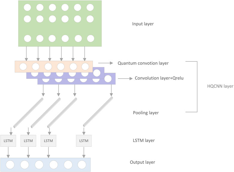
Figure 1. Model structure diagram.

2.1 Quantum classical convolutional neural networks

In the field of weather prediction, the application of time-series prediction usually requires the analysis of large data containing multiple sets of dynamic variables and a high demand for real-time prediction. However, this also poses the challenge that classical computers [38] cannot keep up with changing weather conditions in a real-time manner. In order to improve the accuracy of air quality prediction, this study proposes a quantum classical convolutional neural network (HQCNN) as shown in Figure 2, where a part of the neural network is made into a quantum, and the function of the quantum convolutional layer is consistent with the classical convolutional neural network. In the architecture of the quantum classical convolutional neural network, the network starts with an input layer, followed by a quantum convolutional layer, followed by a classical convolutional layer, then a pooling layer and a fully-connected layer, and finally ends with an output layer, forming a complete processing flow. This design allows the model to extract features from the temporal and spatial dimensions separately, effectively realizing the capture of spatial distribution characteristics of air quality over different time periods. Through this spatio-temporal feature fusion mechanism, the network is able to perform air quality prediction more accurately.

Figure 2

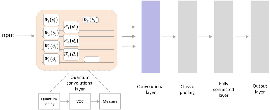
Figure 2. Quantum classical convolutional neural network.

In a quantum neural network, the first task is to transform the input data X into a quantum state. Once the encoding of the information is completed, a series of quantum gates are acted on one or more quantum bits. These quantum gates are responsible for manipulating the input quantum state and converting it into another quantum state through operations such as entanglement and rotation. This process, X → H, i.e., performing quantum feature mapping, where H stands for Hilbert space, is a key step in quantum computation. Specifically, the process of converting a one-dimensional classical vector $x={(x_1,x_2,\dots ,x_n)}^T$ into a quantum state code can be described as shown in Eq. 1 below:

${\mathrm{U}}_{\varphi }(\mathrm{x}):\mathrm{x}\in {\mathbb{R}}^{\mathrm{N}}\to |\varphi \rangle ={\otimes }_{\mathrm{j}=\mathrm{1}}^{\mathrm{N}}{\mathrm{V}}_{\mathrm{j}}\left({\mathrm{c}}_{\mathrm{j}}\left({\mathrm{x}}_{\mathrm{j}}\right)\right)|{\mathrm{0}\rangle }^{\otimes \mathrm{N}}(1)$

When the initial quantum states are all |1⟩ and R_y as V_j, then the quantum state corresponding to x_j is shown in Eq. 2 below:

$|{\varphi }_j\rangle =\cos \left(\frac{x_i}{2}\right)|0\rangle +\sin \left(\frac{x_i}{2}\right)|1\rangle (2)$

The specific representation of the quantum state represented by the array x in tensor product form is shown in Eq. 3 below:

$|\varphi \rangle ={\otimes }_{j=1}^N\cos \left(\frac{x_i}{2}\right)|0\rangle +\sin \left(\frac{x_i}{2}\right)|1\rangle (3)$

The quantum convolutional layer extracts the features or patterns of quantum bits and can be constructed using the unitary gates of any two quantum bits. The quantum convolution kernel designed using VQC performs the unitary transformation U_i on the quantum state, and the U_i operation acts against a pair of neighboring quantum bits as shown in Figure 3.

Figure 3

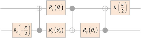
Figure 3. Circuit diagram of quantum convolutional layer.

The design of the baseline VQC is based on the creation of an optimal circuit for the computation of N(α, β, γ) in order to implement the two-qubit VQC from U(4). Here, each unitary matrix in U ∈ (4) can be decomposed in the following way (Eq. 4):

$U=\left(A_1\otimes A_2\right)\cdot N\left(\alpha ,\beta ,\gamma \right)\cdot \left(A_3\otimes A_4\right)(4)$

Where A_j ∈ U(2), ⊗ is the tensor product, and $N(\alpha ,\beta ,\gamma )=\exp \left(i\left[\alpha {\sigma }_x\otimes {\sigma }_x+\beta {\sigma }_y\otimes {\sigma }_y+\gamma {\sigma }_z\otimes {\sigma }_z\right]\right)$. The parameters $\alpha ,\beta ,\gamma \in \mathbb{R}$ are defined as $\alpha =\frac{\pi }{2}-2\theta$, $\beta =2Ø-\frac{\pi }{2}$, and $\gamma =\frac{\pi }{2}-2\lambda$. By using the circuit design illustrated in Figure 3 in conjunction with the regular decomposition technique, it is possible to realize the unitary operations for U ∈ U(4), i.e., VQC. The first quantum convolutional layer can express its output is shown in Eq. 5 below:

$|{\phi }_i\left(\theta \right)\rangle \langle {\phi }_i\left(\theta \right)|=T{r}_{G_i}\left(U_i\left({\theta }_i\right)|{\phi }_{i-1}\rangle \langle {\phi }_{i-1}|U_i{\left({\theta }_i\right)}^{\text{t}}\right)(5)$

Where $T{r}_{G_i}(\cdot )$ denotes the subsystem G_i, U_i is the VQC operation (i.e., quantum convolution), and θ_i is the parameter of the VQC of the ith quantum convolutional layer.

After the quantum transformation of the data, it needs to be measured so that the output quantum state is converted to classical information so that the subsequent part of the classical neural network can process it accordingly. At the end of the variational quantum circuit is the measurement layer, which is used to perform the measurement operation on the quantum bits, and the output quantum states measure the expectation value of each quantum bit. The expectation value is obtained by measuring each quantum bit using the Pauli matrix Z-gate, which is given in the following Eq. 6:

$Z=\left(\begin{array}{cc}\hfill 1\hfill & \hfill 0\hfill \\ \hfill 0\hfill & \hfill -1\hfill \end{array}\right)=|0\rangle \langle 0|-|1\rangle \langle 1|(6)$

After the features X are processed in the quantum convolutional layer, the quantum bits are collapsed into computer-processable bit states. Next, these states are combined with the classical convolutional layer and acted upon by an activation function to generate the output feature map X. This feature map is then fed into the pooling layer, which has the ability to shrink in size for feature compression and refinement. After spreading the feature map X into one-dimensional vectors, the output AQI values are obtained using a fully connected layer decoding. At this stage, the network extracts the key features of the actual data by compressing the two-dimensional input matrix, which ensures that the network is able to accurately transform the input data into the corresponding air quality index and establish an effective mapping from input to output. When the network reaches the expectation, the first phase of network training stops and the next phase of training starts.

2.2 Quantum activation function

In air quality prediction studies, the gradient problem [39] usually arises, making accurate prediction a challenging task. Although existing activation functions [40] have made progress in solving the proposed problem, they often ignore the “dying ReLU problem” of activation functions. In order to solve the problem that gradients in long time series are difficult to propagate in the network and the model cannot effectively learn the long time dependence, this study introduces a quantum activation function (QRELU) in the convolutional layer of the quantum classical convolutional neural network, so that it evaluates the output of the convolution operator, the bias term, and the feature information of the consecutive layers, thus avoiding the gradient problem better and improving the prediction accuracy.

The Quantum Activation Function utilizes a quantum computing approach to provide an innovative solution to the “dying ReLU problem” of the traditional ReLU activation function, ensuring that neurons remain active. By integrating the core principles of quantum computing - superposition and entanglement - the function helps the network to reach a global optimum in the solution process. Utilizing the proposed Leaky RELU method as a baseline, the quantum concepts of superposition and entanglement are incorporated on this basis, thus enabling the function to provide not only positive but also negative solutions. By strategically choosing positive solutions to avoid negative ones, the “dying ReLU” problem is solved in a precisely controlled manner, realizing that only the positive results are retained while the negative effects are eliminated.

Positive solutions of the ReLU function and negative values of the LReLU are chosen as starting points for improvement. Using the principle of quantum entanglement, tensor product operations are performed on the candidate Hilbert state spaces of these two ReLUs (i.e., HRELU) and LReLUs (i.e., HLRELU) as follows Eq. 7:

$H_{\mathit{ReLU}}\otimes H_{\mathit{LReLU}}(7)$

With the Hilbert ReLU-based system in state |α⟩_ReLU and the Hilbert LReLU-based system in state |α⟩_LReLU, the resulting state in the hybrid system will be described by the following Eq. 8:

$|{\alpha \rangle }_{\text{Re}LU}\otimes |{\alpha \rangle }_{L\text{Re}LU}(8)$

In entangled or nonseparable states, the formulas for these product states can be generalized to obtain the following Eq. 9:

$|{\alpha \rangle }_{\mathit{QReLU}}={\displaystyle \sum _{\mathit{ReLU,LReLU}}}{k}_{\mathit{ReLU,LReLU}}|0|{1\rangle }_{\mathit{ReLU}}\otimes |0|{1\rangle }_{\mathit{LReLU}}(9)$

The entangled state of the quantum-based solution is shown in Eq. 10 below:

$|{1\rangle }_{L\text{Re}LU}\otimes |{0\rangle }_{\text{Re}LU}-2|{0\rangle }_{\text{Re}LU}\otimes |{1\rangle }_{L\text{Re}LU}(10)$

In the classical form, the following Eq. 11: can be derived:

$R{\left(\upsilon \right)}_{Q\text{Re}LU}=\phi \times \upsilon -2\upsilon ,\forall \upsilon \le 0(11)$

For positive values (_υ>0), keeping $\mathsf{R}(\upsilon )=\upsilon$, as shown in ReLU, and for negative values, increasing the novelty of the entanglement solution, avoiding the “death of ReLU” by keeping the solution positive with this new quantum state.

2.3 LSTM networks

In this study, according to the encoder-decoder [41] architecture, the HQCNN (Hybrid Quantum Convolutional Neural Network) assumes the role of an encoder, which is responsible for encoding the input data, and the LSTM (Long Short-Term Memory) serves as a decoder to receive these encoded features and interpret them. In a long short-term memory network (LSTM), the forgetting gate is responsible for deciding, with a certain probability, the amount of information that the cell should forget about the state of the hidden unit. Meanwhile, the input gate is responsible for processing the neuron input at the current time step. The output gate, on the other hand, controls the output that the neuron should produce at the current moment. Specifically, the input of the current moment and the hidden unit state of the previous moment together update the cell state through the influence of the forgetting gate and the input gate. The cell then passes the cell state along the time axis in channels with little information decay, allowing the network to effectively preserve long-term time-dependent information, i.e., preserve long-term memory. As for the specific content of the neuron’s output at the current moment, it is selectively controlled by the output gate. In the quantum convolutional classical network, the output produced by the pooling layer will be used as input to the LSTM layer for further processing. The input matrix is compressed and then the extracted features are converted into highly concentrated one-dimensional vectors with time series features. The values of $O_{(t,\dots ,t-D)}^c$ and $O_{(t,\dots ,t-D)}^f$ for the D days between time t are the model inputs, and the prediction target is the AQI for the N days after the time t (D and N are the set time windows). w is the weight, h is the hidden layer information, and b is the bias. Figure 4 of the classical LSTM network is shown below and the following equations are used to represent the training process of the LSTM.

i. The LSTM first selectively forgets some past AQI data information and other factors as shown in Eq. 12 below:

$f_t=\sigma \left(W_f\left[h_{t-1},x_t\right]+b_f\right)(12)$

ii. The new information selected to be deposited during the update of the cell state comes from two parts, as shown in Eq. 13 below. The sigmoid layer of the “input threshold” is responsible for filtering out the information that needs to be updated, while the tanh layer generates a new vector of candidate values as shown in Eq. 14 below:

$i_t=\sigma \left(W_i\left[h_{t-1},x_t\right]+b_i\right)(13)$

$C_t^{\prime }=\tanh \left(W_C\left[h_{t-1},x_t\right]+b_t\right)(14)$

iii. Update the previous state as shown in Eq. 15 below:

$C_t=f_t{c}_{t-1}+i_t{C}_t^{\prime }(15)$

iv. Finally, the output information is determined as shown in Eqs 16, 17 below, i.e., the predicted AQI:

$o_t=\sigma \left(W_o\left[h_{t-1},x_t\right]+b_0\right)(16)$

$h_t=o_t\tanh \left(C_t\right)(17)$

Figure 4

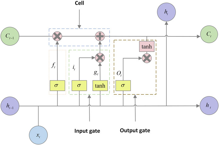
Figure 4. LSTM cell.

2.4 Algorithmic flow

In this study, an algorithm for optimizing quantum hybrid neural networks with quantum activation functions is proposed, which integrates a quantum classical hybrid network with a long short-term memory (LSTM) network to create a novel hybrid model. In this model, it is mainly composed of two parts: feature extraction and air quality prediction. The algorithm accelerates the learning rate of the neural network by quantizing part of the convolutional layer of the convolutional neural network, taking full advantage of the efficient parallel processing capability of quantum computing as well as the deep extraction of features. The long and short-term memory network can retain useful feature information for a long time by utilizing forgetting gates, input gates, and output gates, and has good time series data processing capability. Therefore, the Hybrid Quantum Convolutional Neural Network (HQCNN) partially serves the purpose of automatic extraction of features which are subsequently passed to the LSTM network for accurate air quality prediction.

The feature extraction stage consists of an input layer, a quantum convolutional layer, a classical convolutional layer, and a classical pooling layer. Among them, the convolution filter of the quantum convolution layer consists of a VQC, in which a four-quantum-bit variational circuit is used instead of a convolution kernel to realize the extraction of features, and the variational circuit layer of the VQC is used to perform a quantum state you transformation on the encoded data, and then this result is output to form the corresponding output feature data after measurement. Then after the classical convolutional layer of convolutional calculation, the convolutional kernel is slid with the data in steps for the convolutional operation, and then this result is summed with the bias of this convolutional layer to realize the nonlinear output using the quantum activation function. This is then followed by a pooling layer using maximum pooling method for data reduction and further feature extraction.

Among them, the convolution part of the classical convolutional layer uses the “QRELU” activation function to evaluate the result of the convolution operation, the bias term and the feature information of the successive layers, and the output feature information of the convolutional layer is evaluated as shown in Eqs 18, 19 below:

$a_k^i=Qrelu\left(z_k^i\right)=\left\{\begin{array}{c}{z}_k^i,z_k^i\ge 0\hfill \\ \alpha z_k^i-2z_k^i,z_k^i\le 0\end{array}\right.(18)$

$\left\{\begin{array}{c}{a}_k^i=Qrelu\left(z_k^i\right)\hfill \\ z_k^i={\sum }_{k=1}{a}_k^{i-1}\otimes r_{mk}^i+b_k^i\end{array}\right.(19)$

where $a_k^{i-1}$is the input of the convolution filter, $a_k^i$ is the output, r is the convolution kernel, b is the bias term, and ⊗ denotes the convolution operator.

These features are then passed to the LSTM network in a one-to-one fashion, thus entering the air quality prediction part in order to further exploit the time-dependent features. At the end of the network, a deep neural network containing a single hidden layer is used as a fully-connected layer that constitutes the output layer of the HQCNN-LSTM network model, responsible for the final fitting and prediction of the data. The output of the model is the predicted value at time point t, giving the framework a higher sequential prediction capability. Figure 5 illustrates the specific flow of the method.

Figure 5

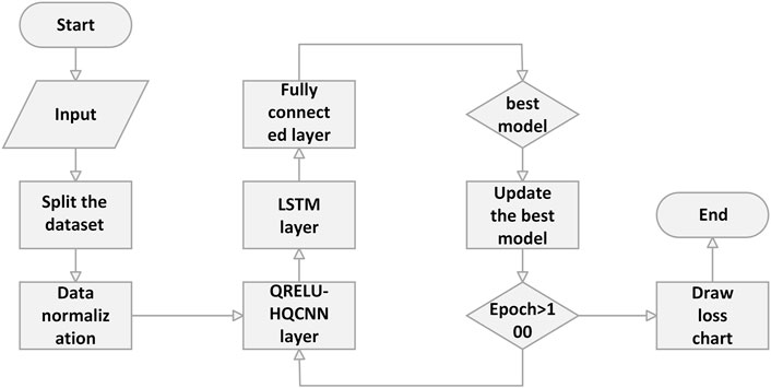
Figure 5. Presentation of model flow charts.

The specific stages of the air quality prediction algorithm based on quantum activation function optimization hybrid quantum neural network (QRELU-HQCNN-LSTM) are as follows:

Step 1: The air quality time series dataset is input, containing daily measured data related to PM2.5, PM10, SO2, CO, NO2, O3, etc.

Step 2: Dividing the dataset, in this paper, 76% of the dataset is used as the training set and 24% is used as the test set.

Step 3: Data normalization [42]. In order to eliminate the influence of different dimensions, Min-Max Scalering normalization is used to scale the data to the range [0,1].

Step 4: HQCCN layer, which sends the processed data to the quantum convolutional layer for feature extraction, prepares the quantum state, and obtains the training set and test set; constructs a hybrid quantum-classical convolutional neural network and uses the QRELU activation function in the convolutional layer; and sets the values of the batch size, epoch, and the learning rate; the quantum system undergoes the You transformation; and then goes through the classical part of the output to obtain the data output1.

Step 5: The LSTM layer, which inputs the data output1 to the LSTM layer and uses its hidden state to compute the time series to get the output data output2. Meanwhile, the optimal model best-model. h5 is automatically saved during the training process and the optimal model is called when in the subsequent prediction.

Step 6: The fully connected layer, which inputs the data output2 computed by the LSTM layer to the fully connected layer to get output3.

Step 7: To determine whether to end, where the end condition is to complete the set epoch. If the number of times reaches the standard, then end the model training, otherwise, continue to train the model in accordance with step 4.

Step 8: End.

3 Experimentation and analysis

3.1 Experimental data and indicators

The data for this study were obtained from the historical air quality data of Shanghai, Chengdu, Shenzhen and Hangzhou published by Weatherpost.com, and the samples were selected from the three air pollutant datasets of Shanghai, Chengdu, and Shenzhen from 2015-01-01 2016-12-31, and the air pollutant dataset of Hangzhou from 2022-01-01 2023-12-31. Among them, the Shanghai, Chengdu and Shenzhen datasets each have 731 sets of data, and the Hangzhou dataset has a total of 720 sets of data, in which the daily measured PM2.5, PM10, SO2, CO, NO2, O3, and AQI indexes are used as the input parameters, whereas the AQI indexes are used as the prediction targets of the model.

Since the time series data was collected manually, missing data, data redundancy and some unforeseen problems inevitably occurred during the data collection process. The air quality data collected for these cities showed the same problems, therefore, data preprocessing was done before the experiment started.

i. Handling of missing values

During the collection of air quality data, some dates corresponding to the various indices were missing, and the mean-filling approach was adopted for continuous variables, and the median-filling approach was adopted for discrete variables, in which the missing data were filled accordingly. For some irrelevant or obviously low relevance feature variables, such as the AQI data of the day, air quality level data, etc., a direct deletion method was adopted so as not to affect the learning and generalization ability of the subsequent model.

ii. Handling of outliers

In the process of data analysis, it is common to encounter data points that are outside the predefined reasonable range or exhibit significant outliers. By applying the method based on the median absolute deviation and combining it with the calculation of the sum of the distances of each observation from the mean, we are able to effectively identify and deal with the outliers, thus ensuring the robustness and reliability of the data analysis.

The trend of air quality index (AQI) and air pollutant concentration over time for each dataset collected in this paper after the above two steps of preprocessing is shown in Figure 6 below.

Figure 6

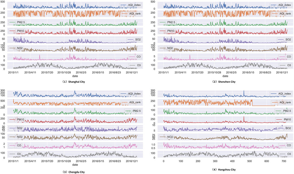
Figure 6. Trend map of data sets.

After pre-preprocessing the air quality time-series dataset of the four cities, the QRELU-HQCNN-LSTM model has a high sensitivity to the data scale due to the different orders of magnitude of the air quality data. In order to avoid problems such as slow convergence speed of the model affected by large data variations, normalization of the dataset according to Eq. 20 is necessary.

$X_n=\frac{X-X_{\min }}{X_{\max }-X_{\min }}(20)$

Air quality prediction is essentially a regression problem [43]. In order to effectively evaluate the performance of the prediction model, three key metrics were selected in this study: root mean square error (RMSE), mean absolute error (MAE), and mean absolute percentage error (MAPE). These metrics are used to quantify the accuracy of the model’s predictions; the smaller their value, the more accurate the model’s predictions. The relevant equations are shown in Eqs 21–23 below:

$RMSE=\sqrt{\frac{1}{N}{\displaystyle \sum _{n=1}^N}{\left(y_n-\stackrel{\wedge }{y}n\right)}^2}(21)$

$MAE=\frac{1}{N}{\displaystyle \sum _{n=1}^N}\left|y_n-\stackrel{\wedge }{y}n\right|(22)$

$MAPE=\frac{1}{N}{\displaystyle \sum _{n=1}^N}\frac{\left|\begin{array}{c}\hfill \hfill \\ \hfill y_n-\stackrel{\wedge }{y}n\hfill \end{array}\right|}{y_n}(23)$

where n represents the number of samples in the time series, y_n represents the actual observations in the time series forecast, and ${\widehat{y}}_n$ represents the corresponding predicted values in the time series forecast.

3.2 Data correlation analysis

In this experiment, Pearson correlation coefficient [44] (p = 0.05) was used to correlate the data characteristics of the four air quality datasets, and from the correlation coefficient plots of each factor of the air quality data (Figure 7), it can be seen that there are positive correlations between various pollutants, and these relationships can be quantified to obtain specific correlation coefficient values. These correlation coefficient values can help us understand the degree of correlation between different pollutants and provide important references for further air quality studies. After the preprocessed data were evaluated for feature importance and correlation analysis, a total of 731 data from Shanghai, Chengdu and Shenzhen datasets and 720 data from Hangzhou dataset used in this study were screened, and the first 76% of the dataset was divided as the training set with the remaining 24% as the test set.

Figure 7

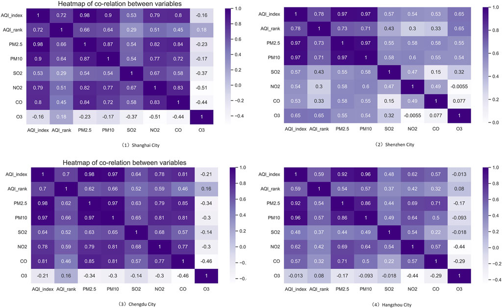
Figure 7. Plot of correlation coefficients.

3.3 Experimental environment and parameters

In this section, we evaluate the performance of the proposed QRELU-HQCNN-LSTM model against other models such as CNN-LSTM; the parameters of the QRELU optimization model are set as follows: the model combines a convolutional layer for the QRELU activation function and an LSTM layer for the Tanh activation function, with a number of filters of 16, a learning rate of 0.004, and a number of training rounds of 100. The batch training size is 256, the optimizer is Adam and the loss function used is RMSE (Root Mean Square Error). The parameter selection method is grid search method. All experiments were performed on a 12th Gen Intel(R) Core(TM) i9-12900H, 2.50 GHz, GTX1660Ti GPU computer. All models were built on the Keras 2.2.4 framework and the code was edited using the Python 3.9 based Juypter Notebook.

3.4 Experimental results and analysis

Firstly, in order to prove the effectiveness of the QRELU-HQCNN-LSTM algorithm for predicting air quality, it is compared and then tested in detail, which is based on quantum theory and re-optimized on the basis of classical neural networks. The performance of the QRELU-HQCNN-LSTM algorithm under the same conditions on different datasets is then carefully verified and proved that it does have some advantages. In this section of experiments the corresponding models and their variant network CNN-LSTM models are built on the datasets of Shanghai, Chengdu, Shenzhen and Hangzhou for comparison. LSTM, CNN-LSTM, QRELU-CNN-LSTM and QRELU-HQCNN-LSTM models are selected for predicting the air quality and the prediction results are compared and analyzed, and the prediction results of Shanghai City, Chengdu City, Shenzhen City, and Hangzhou City are shown in Figures 8–11, respectively.As can be seen from the above figure, the overall trend of the predicted and actual values of each prediction model is the same, when the data curve has a large downward trend, the other models can not fit well, and the predicted values of the QRELU-HQCNN-LSTM model proposed in this paper are closer to the real values. The main reason is that HQCNN can learn better from the original input sequence, thus avoiding the error caused by manual extraction of features; adding QRELU activation function to HQCNN can more effectively avoid the “death” problem, thus the QRELU-HQCNN-LSTM algorithm has a higher prediction accuracy, higher output curve fitting, and higher prediction accuracy. The QRELU-HQCNN-LSTM algorithm has higher prediction accuracy and higher output curve fit.

Figure 8

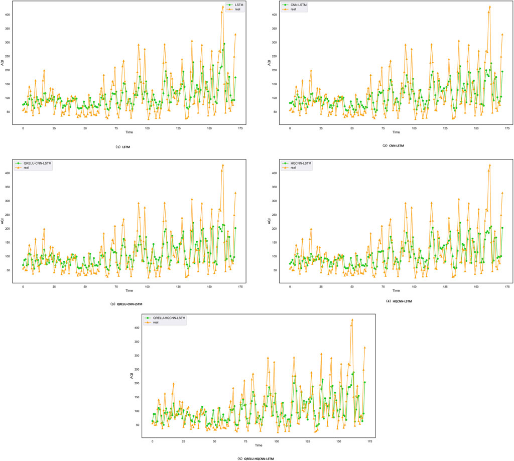
Figure 8. Prediction effect of different models in Shanghai, the yellow curve indicates the trend of the actual air quality data in the Shanghai dataset, and the green curve indicates the prediction trend of different models; when the trend of the predicted data in the yellow line and the trend of the actual data in the green line are close to each other, it means that the model is more accurate and the prediction effect is more excellent.

Figure 9

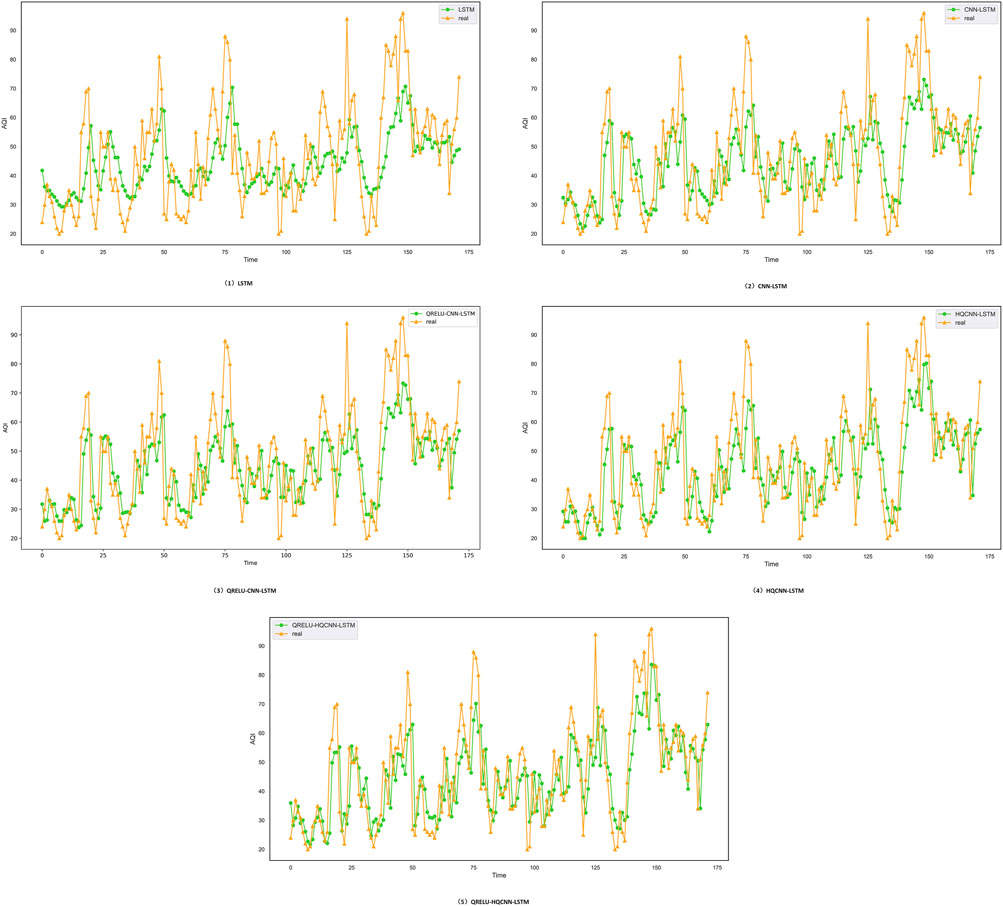
Figure 9. Prediction effect of different models in Shenzhen, the yellow curve indicates the trend of the actual air quality data in the Shenzhen dataset, and the green curve indicates the prediction trend of different models; when the trend of the predicted data in the yellow line and the trend of the actual data in the green line are close to each other, it means that the model is more accurate and the prediction effect is more excellent.

Figure 10

Figure 10. Prediction effect of different models in Chengdu, where: the yellow curve indicates the trend of the actual air quality data in the dataset of Chengdu, and the green curve indicates the predictive trend of different models; when the predictive data trend of the yellow line and the trend of the actual data of the green line are close to each other, then it means that the model is more accurate, and the prediction effect is more excellent; in short, the closer the predictive data is to the actual data, the higher the accuracy of the model. In short, the closer the predicted data are to the actual data, the higher the accuracy of the model.

Figure 11

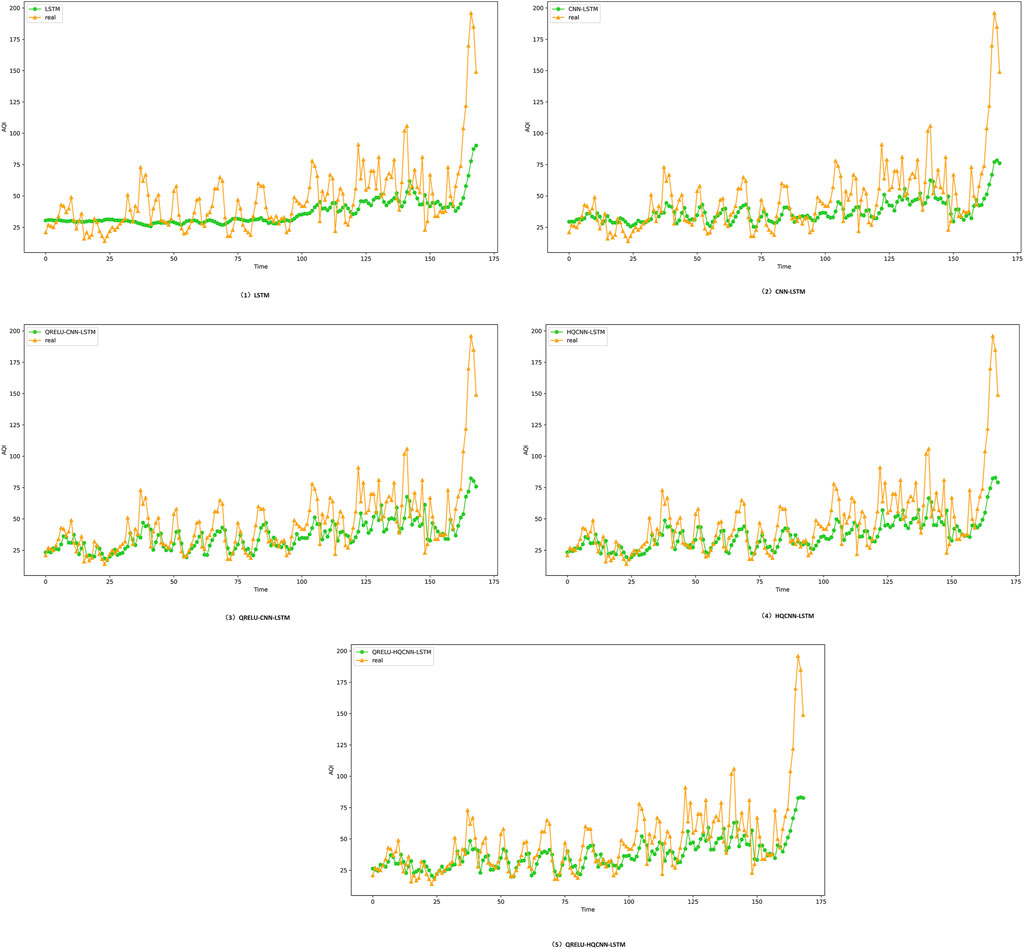
Figure 11. Prediction effect of different models in Hangzhou, where: the yellow curve indicates the trend of the actual air quality data in the dataset of Hangzhou, and the green curve indicates the predictive trend of different models; when the predictive data trend of the yellow line and the trend of the actual data of the green line are close to each other, then it means that the model is more accurate, and the prediction effect is more excellent; in short, the closer the predictive data is to the actual data, the higher the accuracy of the model. In short, the closer the predicted data are to the actual data, the higher the accuracy of the model.

In order to better reflect the superiority of the prediction accuracy of the QRELU-HQCNN-LSTM model proposed in this paper, the RMSE, MAPE and MAE of the different models on the corresponding datasets are listed in Table 1, Table 2, Table 3, and Table 4, respectively. The RMSE, MAE, and MAPE stand for the root-mean-square-error, the mean-absolute error, and the mean-absolute-percentage-error of the prediction, respectively. By comparing the data in the three tables, it is clear that the HQCNN-LSTM model outperforms the CNN-LSTM model in terms of performance. Specifically, in Table 1, the HQCNN-LSTM model reduces the RMSE by 0.5223, the MAPE by 0.0158 percentage points, and the MAE by 0.5423 accordingly; Table 2 shows that the model reduces the RMSE by 1.1718, the MAPE by 0.0169 percentage points, and the MAE by 0.9521; and in Table 3, the RMSE is reduced by 0.4212, the MAPE is reduced by 0.0063 percentage points, and the MAE is reduced by 0.4874; while in Table 4, the RMSE is reduced by 1.1992, the MAPE is reduced by 0.0248 percentage points, and the MAE is reduced by 0.8288. This suggests that quantum entanglement enhances the performance of CNN-LSTM models in extracting localized data important features, which improves the prediction effect and accuracy of the model. Compared with the HQCNN-LSTM model, the QRELU-HQCNN-LSTM model exhibits a more significant enhancement, with a reduction of 0.7407 in RMSE, 0.0116% in MAPE, and 0.5091 in MAE in Table 1; in Table 2, a reduction of 1.5597 in RMSE, 0.0598% in MAPE, and 2.1794; in Table 3, RMSE decreased by 1.3227, MAPE decreased by 0.0024%, and MAE decreased by 0.4311; and in Table 4, RMSE decreased by 0.0997, MAPE decreased by 0.003%, and MAE decreased by 0.1275. This indicates that the QRELU-HQCNN-LSTM model is better in fitting the anomalies and It also improves the model’s ability to fit and predict the true value of AQI. Compared with the CNN-LSTM model, the QRELU-HQCNN-LSTM model shows significant improvement in prediction accuracy. The reason behind this achievement is that the QRELU-HQCNN-LSTM algorithm is more capable of optimization, which helps the model to obtain a better network structure and learning speed.

Table 1

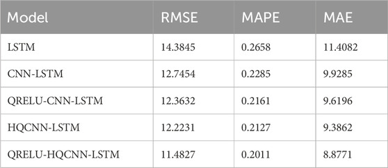
Table 1. Shenzhen city - comparison of prediction results of different models.

Table 2

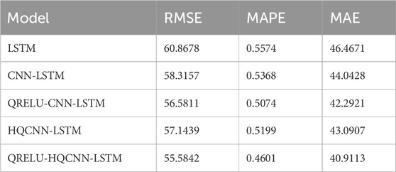
Table 2. Shanghai - comparison of prediction results of different models.

Table 3

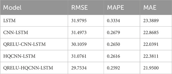
Table 3. Chengdu city-comparison of prediction results of different models.

Table 4

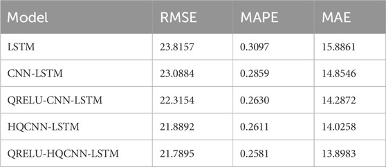
Table 4. Hongzhou city-comparison of prediction results of different models.

In order to further demonstrate the superiority of the quantum activation function optimized prediction model proposed in this paper, which can perform air quality prediction more accurately, four datasets, namely, Shanghai City, Chengdu City, Shenzhen City, and Hangzhou City, are selected for demonstration. The effect of activation function on the performance of the HQCNN-LSTM algorithm is explored, and it is observed that the selection of different activation functions for the optimization of the quantum hybrid neural network will present different results. In this section, the performance of the QRELU activation function under the same conditions is carefully verified using different datasets, and it is proved that it does have certain advantages and can effectively solve the “death problem” of the RELU function. By looking at Figure 12, the predicted values and the true values of the Shanghai dataset are compared with those of the Shenzhen, Chengdu and Hangzhou datasets, as shown in Figures 13–15, respectively.

Figure 12

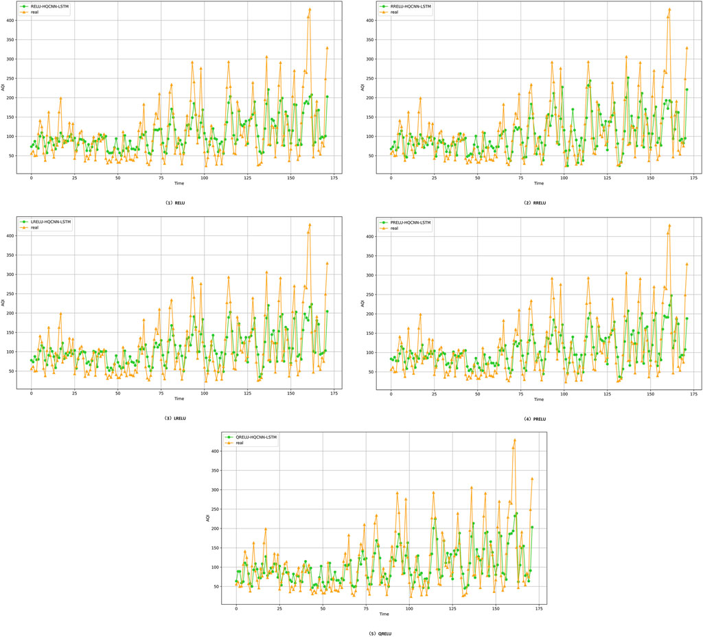
Figure 12. Prediction results of optimization model with different activation functions in Shanghai city, the yellow curve indicates the trend of the actual air quality data in the Shanghai dataset, and the green curve indicates the trend of the data prediction using different activation function optimization HQCNN-LSTM models; when the trend of the predicted data in the yellow line is closer to the trend of the actual data in the green line, it means that the model is more accurate, and the prediction results are more excellent. In short, the closer the predicted data is to the actual data, the higher the accuracy of the model.

Figure 13

Figure 13. Prediction results of optimization model with different activation functions for Shenzhen city, the yellow curve indicates the trend of the actual air quality data in the Shenzhen dataset, and the green curve indicates the trend of the data prediction using different activation function optimization HQCNN-LSTM models; when the trend of the predicted data in the yellow line is closer to the trend of the actual data in the green line, it means that the model is more accurate and the prediction results are better. In short, the closer the predicted data is to the actual data, the higher the accuracy of the model.

Figure 14

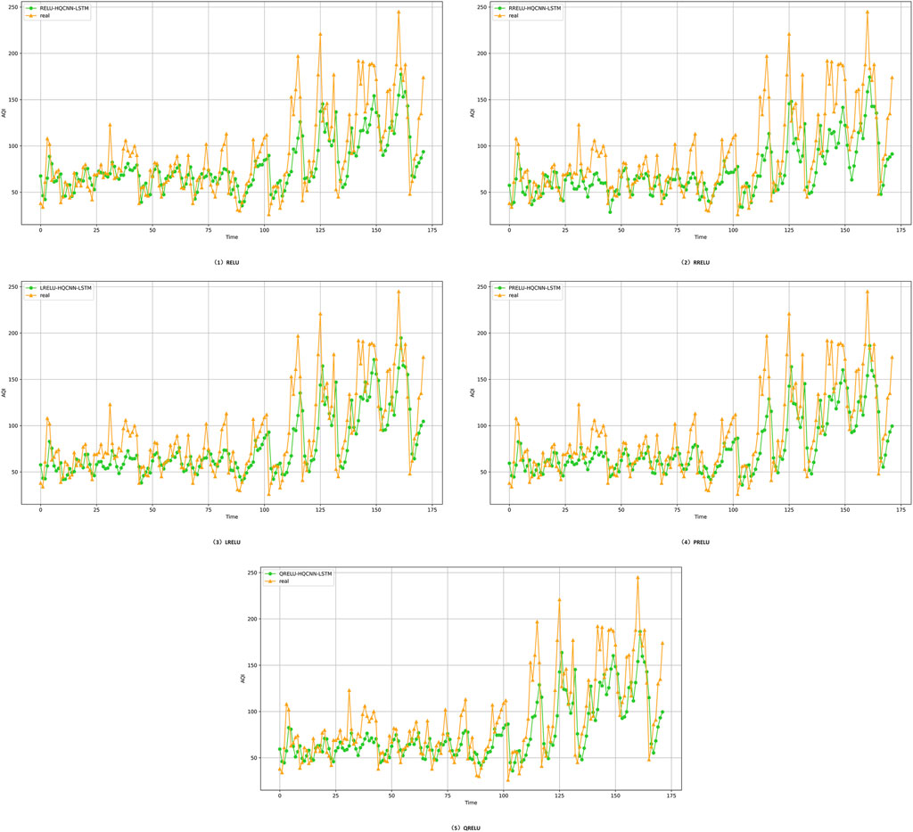
Figure 14. Prediction results of optimization model with different activation functions for Chengdu city, the yellow curve indicates the trend of the actual air quality data in the dataset of Chengdu city, and the green curve indicates the trend of the data prediction using different activation functions of the optimized hybrid quantum neural network model; when the trend of the predicted data in the yellow line is closer to the trend of the actual data in the green line, it means that the model is more accurate and the prediction is more excellent. In short, the closer the predicted data are to the actual data, the higher the accuracy of the model.

Figure 15

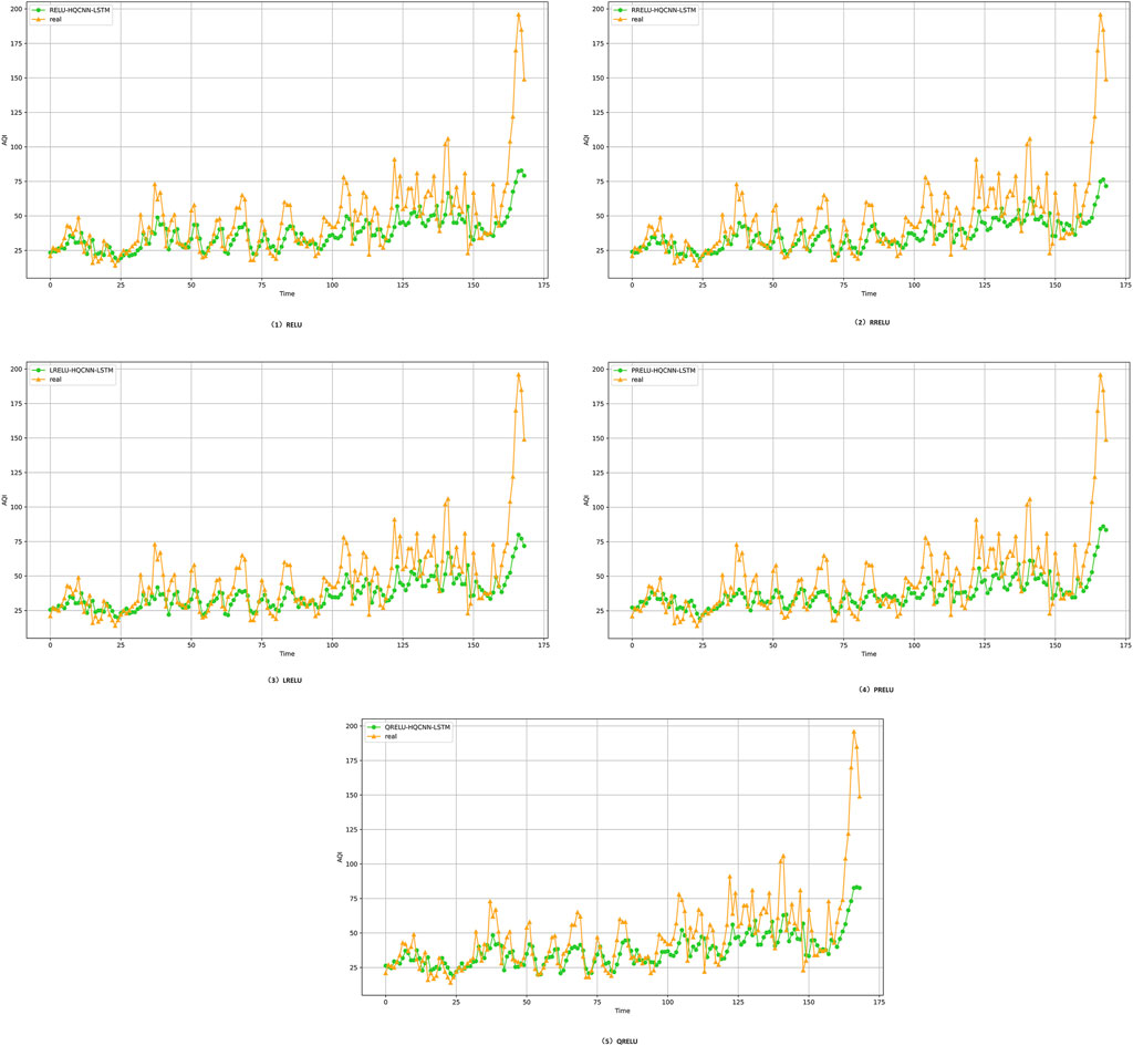
Figure 15. Prediction results of different activation function optimization models in Hangzhou, where: the yellow curve indicates the trend of the actual air quality data in the Hangzhou dataset, and the green curve indicates the trend of the data prediction using different activation functions to optimize the hybrid quantum neural network model; when the trend of the predicted data in the yellow line is closer to the trend of the actual data in the green line, it means that the model is more accurate and the prediction is better. In short, the closer the predicted data are to the actual data, the higher the accuracy of the model.

From the data in Tables 5–8, it is obvious that the QRELU activation function shows the best performance in all the indexes, in Table 5, the RMSE, MAPE, and MAE reach 11.4827,0.2011%,8.8771 respectively; in Table 6, the RMSE, MAPE, and MAE reach 55.5842, 0.4601%, and 40.9113; in Table 7, RMSE, MAPE, and MAE reach 29.7534, 0.2592%, and 21.9500, respectively; and in Table 8, RMSE, MAPE, and MAE reach 21.7895, 0.2581%, and 13.8983, respectively; in comparison, the model optimized by QRELU activation function performs optimally in these indicators. Among the various activation functions, the QRELU-HQCNN-LSTM model has the highest prediction accuracy, and most of its predicted values match with the actual values, and the QRELU activation function obviously has a more obvious impact on the improvement of model performance. This indicates that the QRELU activation function solves the “dying problem” in the traditional activation function to a certain extent, and improves the fitting ability of the HQCNN-LSTM model to the real value of the air quality, which further improves the accuracy and stability of the model.

Table 5

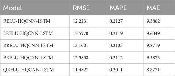
Table 5. Shenzhen City—comparison of the results of indicators with different activation functions.

Table 6

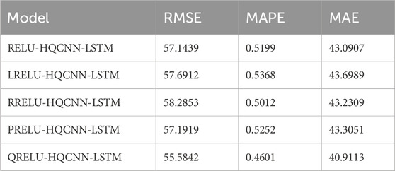
Table 6. Shanghai—comparison of indicator results for different activation functions.

Table 7

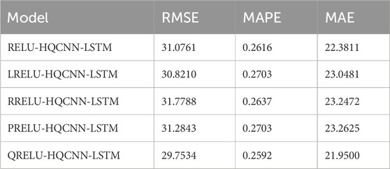
Table 7. Chengdu city—comparison of indicator results for different activation functions.

Table 8

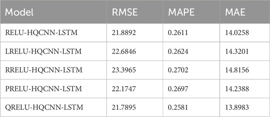
Table 8. Hangzhou city - comparison of indicator results for different activation functions.

The QRELU-HQCNN-LSTM model highlights the advantages of quantum computing in handling complex data and problems. The superiority of hybrid quantum neural networks is demonstrated when dealing with real data, and although it may be more time-consuming at runtime, the advanced features of quantum computing enable higher prediction accuracy and stronger data processing. When dealing with air quality data, the quantum superposition and entanglement states of quantum computing give the HQCNN-LSTM model a unique advantage in parallel processing and complex problem solving, and it can more accurately fit the real values; at the same time, the introduction of the quantum activation function not only solves the “dying problem” of the traditional activation function, but also improves the performance of the hybrid quantum neural network on the data. At the same time, the introduction of quantum activation function not only solves the “dying problem” of traditional activation function, but also improves the sensitivity of hybrid quantum neural network to the data and the depth of feature extraction, which further enhances the accuracy and stability of the model.

4 Conclusion

This paper focuses on the prediction of a typical air quality index, i.e., the prediction of future AQI based on historical air quality data. In this paper, a HQCNN-LSTM model based on QRELU activation function is proposed, aiming at extracting the spatial features of the air quality index over different time periods using quantum convolutional neural network. The model is improved by the quantum activation function, which effectively avoids the dead ReLU problem and improves the stability and performance performance of the model. Subsequently, the temporal features of the air quality index are extracted using LSTM network, which realizes the effective fusion of spatio-temporal information. By simulating the datasets of three cities, this paper demonstrates that the proposed model can significantly improve the prediction accuracy of the AQI. By comparing the error metrics RMSE, MAPE and MAE, it is clearly demonstrated that the QRELU-HQCNN-LSTM model outperforms the LRELU-HQCNN-LSTM, RRELU-HQCNN-LSTM and PRELU-HQCNN-LSTM models in terms of prediction performance. This demonstrates the significant value and practical significance of the model used in this paper in air quality prediction.

Data availability statement

The datasets presented in this article are not readily available because This dataset is suitable for air quality prediction. Requests to access the datasets should be directed to http://www.tianqihoubao.com/.

Author contributions

YD: Supervision, Writing–original draft. FL: Methodology, Writing–original draft, Writing–review and editing. TZ: Formal Analysis, Investigation, Writing–review and editing. RY: Writing–review and editing.

Funding

The author(s) declare that financial support was received for the research, authorship, and/or publication of this article. This work was supported by National Natural Science Foundation of China (No. 61772295), Key Projects of Chongqing Natural Science Foundation Innovation Development Joint Fund (CSTB2023NSCQ-LZX0139), Open Fund of Advanced Cryptography and System Security Key Laboratory of Sichuan Province (Grant No. SKLACSS–202208) and Technology Research Program of Chongqing Municipal Education Commission (Grant no. KJZD-M202000501).

Acknowledgments

The authors are grateful for the important technical help given by colleagues in the laboratory and the fund support.

Conflict of interest

The authors declare that the research was conducted in the absence of any commercial or financial relationships that could be construed as a potential conflict of interest.

Publisher’s note

All claims expressed in this article are solely those of the authors and do not necessarily represent those of their affiliated organizations, or those of the publisher, the editors and the reviewers. Any product that may be evaluated in this article, or claim that may be made by its manufacturer, is not guaranteed or endorsed by the publisher.

References

1. Kyrkilis G, Chaloulakou A, Kassomenos PA. Development of an aggregate air quality index for an urban mediterranean agglomeration: relation to potential health effects. Environ Int (2007) 33:670–6. doi:10.1016/j.envint.2007.01.010

PubMed Abstract | CrossRef Full Text | Google Scholar

2. Poursafa P, Mansourian M, Motlagh M-E, Ardalan G, Kelishadi R. Is air quality index associated with cardiometabolic risk factors in adolescents? the caspian-iii study. Environ Int (2014) 134:105–9. doi:10.1016/j.envres.2014.07.010

PubMed Abstract | CrossRef Full Text | Google Scholar

3. Wen X-J, Balluz L, Mokdad A. Association between media alerts of air quality index and change of outdoor activity among adult asthma in six states, brfss, 2005. J. Community Health (2007) 33:670–676. doi:10.1007/s10900-008-9126-4

CrossRef Full Text | Google Scholar

4. Akimoto H. Global air quality and pollution. Science (2003) 302:1716–9. doi:10.1126/science.1092666

PubMed Abstract | CrossRef Full Text | Google Scholar

5. Jones A. Indoor air quality and health. Atmos Environ (1999) 33:4535–64. doi:10.1016/S1352-2310(99)00272-1

CrossRef Full Text | Google Scholar

6. Jones A. The impact of air quality on tourism: the case of Hong Kong. Pac Tourism Rev (2001) 5:69–74.

Google Scholar

7. Dinda S, Coondoo D, Pal M. Air quality and economic growth: an empirical study. Ecol Econ (2000) 34:409–23. doi:10.1016/S0921-8009(00)00179-8

CrossRef Full Text | Google Scholar

8. Hui Z, Bin L, Zhuo-qun Z. Short-term wind speed forecasting simulation research based on arima-lssvm combination method. In: 2011 International Conference on Materials for Renewable Energy I& Environment (IEEE); 20-22 May 2011; Shanghai, China (2011). p. 20–2.

Google Scholar

9. Russo A, Raischel F, Lind PG. Air quality prediction using optimal neural networks with stochastic variables. Atmos Environ (2013) 79:822–30. doi:10.1016/j.atmosenv.2013.07.072

CrossRef Full Text | Google Scholar

10. Yang W, Deng M, Xu F, Wang H. Prediction of hourly pm2. 5 using a space-time support vector regression model. Atmos Environ (2018) 181:12–9. doi:10.1016/j.atmosenv.2018.03.015

CrossRef Full Text | Google Scholar

11. Tian Y, Xu Y-P, Wang G. Agricultural drought prediction using climate indices based on support vector regression in xiangjiang river basin. Sci Total Environ (2018) 622:710–20. doi:10.1016/j.scitotenv.2017.12.025

PubMed Abstract | CrossRef Full Text | Google Scholar

12. Chen H, Guan M, Li H. Air quality prediction based on integrated dual lstm model. IEEE Access (2021) 9:93285–97. doi:10.1109/ACCESS.2021.3093430

CrossRef Full Text | Google Scholar

13. Kareva Z, Suykens JA. Transductive lstm for time-series prediction: an application to weather forecasting. Neural Networks (2020) 125:1–9. doi:10.1016/j.neunet.2019.12.030

PubMed Abstract | CrossRef Full Text | Google Scholar

14. Zhang J, Li S. Air quality index forecast in beijing based on cnn-lstm multi-model. Chemosphere (2022) 308:136180. doi:10.1016/j.chemosphere.2022.136180

PubMed Abstract | CrossRef Full Text | Google Scholar

15. Frolov AV. Can a quantum computer be applied for numerical weather prediction? Russ Meteorology Hydrol (2017) 42:545–53. doi:10.3103/s1068373917090011

CrossRef Full Text | Google Scholar

16. Shapiro J. Genetic algorithms in machine learning. Choice Rev Online (1989) 27:27–0936.

Google Scholar

17. Dunjko V, Briegel HJ. Machine learning and artificial intelligence in the quantum domain: a review of recent progress. Rep Prog Phys (2018) 81:074001. doi:10.1088/1361-6633/aab406

PubMed Abstract | CrossRef Full Text | Google Scholar

18. Flurin E, Hacohen-Gourgy S, Siddiqi I. Using a recurrent neural network to reconstruct quantum dynamics of a superconducting qubit from physical observations. Phys Rev X (2020) 10:011006. doi:10.1103/PhysRevX.10.011006

CrossRef Full Text | Google Scholar

19. Panchi L, Shiyong L. Learning algorithm and application of quantum bp neural networks based on universal quantum gates. J Syst Eng Elect (2018) 19:167–74. doi:10.1016/S1004-4132(08)60063-8

CrossRef Full Text | Google Scholar

20. Khellal A, Ma H, Fei Q. Convolutional neural network based on extreme learning machine for maritime ships recognition in infrared images. Sensors (2018) 18:1490. doi:10.3390/s18051490

PubMed Abstract | CrossRef Full Text | Google Scholar

21. Sharma K, Cerezo M, Cincio L, Coles PJ. Trainability of dissipative perceptron-based quantum neural networks. Phys Rev Lett (2022) 128:180505. doi:10.1103/PhysRevLett.128.180505

PubMed Abstract | CrossRef Full Text | Google Scholar

22. Jeswal SK, Chakraverty S. Recent developments and applications in quantum neural network: a review. Arch Comput Methods Eng (2019) 26:793–807. doi:10.1007/s11831-018-9269-0

CrossRef Full Text | Google Scholar

23. Chen SY-C, Yoo S, Fang Y-LL. Quantum long short-term memory. In: ICASSP 2022 - 2022 IEEE International Conference on Acoustics, Speech and Signal Processing (ICASSP) (IEEE); 22-27 May 2022; Singapore (2022). p. 1748.

CrossRef Full Text | Google Scholar

24. Mitarai K, Negoro M, Kitagawa M, Fujii K. Quantum circuit learning. Phys Rev A (2018) 98:032309. doi:10.1103/PhysRevA.98.032309

CrossRef Full Text | Google Scholar

25. Gong C, Zhou N, Xia S, Huang S. Quantum particle swarm optimization algorithm based on diversity migration strategy. Future Generation Comp Syst (2024) 157:445–58. doi:10.1016/j.future.2024.04.008

CrossRef Full Text | Google Scholar

26. Gong L-H, Ding W, Li Z, Wang Y-Z, Zhou N-R. Quantum k-nearest neighbor classification algorithm via a divide-and-conquer strategy. Adv Quan Tech (2024):2300221. doi:10.1002/qute.202300221

CrossRef Full Text | Google Scholar

27. Zhou N-R, Zhang T-F, Xie X-W, Wu J-Y. Hybrid quantum–classical generative adversarial networks for image generation via learning discrete distribution. Signal Processing: Image Commun (2022) 605:116891. doi:10.1016/j.image.2022.116891

CrossRef Full Text | Google Scholar

28. Cong I, Choi S, Lukin MD. Quantum convolutional neural networks. Nat Phys (2019) 15:1273–8. doi:10.1038/s41567-019-0648-8

CrossRef Full Text | Google Scholar

29. Herrmann J, Llima SM, Remm A, Zapletal P, McMahon NA, Scarato C, et al. Realizing quantum convolutional neural networks on a superconducting quantum processor to recognize quantum phases. Nat Commun (2022) 13:4144. doi:10.1038/s41467-022-31679-5

PubMed Abstract | CrossRef Full Text | Google Scholar

30. Gong L-H, Pei J-J, Zhang T-F, Zhou N-R. Quantum convolutional neural network based on variational quantum circuits. Opt Commun (2024) 550:129993. doi:10.1016/j.optcom.2023.129993

CrossRef Full Text | Google Scholar

31. Paquet E, Soleymani F. Quantumleap: hybrid quantum neural network for financial predictions. Expert Syst Appl (2022) 195:116583. doi:10.1016/j.eswa.2022.116583

CrossRef Full Text | Google Scholar

32. Ceschini A, Rosato A, Panella M. Hybrid quantum-classical recurrent neural networks for time series prediction. In: 2022 International Joint Conference on Neural Networks (IJCNN) (IEEE); 18-23 July 2022; Padua, Italy (2022). p. 353.

CrossRef Full Text | Google Scholar

33. Hong Y-Y, Rioflorido CLPP, Zhang W. Hybrid deep learning and quantum-inspired neural network for day-ahead spatiotemporal wind speed forecasting. Expert Syst Appl (2024) 241:122645. doi:10.1016/j.eswa.2023.122645

CrossRef Full Text | Google Scholar

34. Cerezo M, Arrasmith A, Babbush R, Benjamin SC, Endo S, Fujii K, et al. Variational quantum algorithms. Nat Rev Phys (2021) 3:625–44. doi:10.1038/s42254-021-00348-9

CrossRef Full Text | Google Scholar

35. Bravo-Prieto C. Quantum autoencoders with enhanced data encoding. Machine Learn Sci Tech (2021) 2:035028. doi:10.1088/2632-2153/ac0616

CrossRef Full Text | Google Scholar

36. Greff K, Srivastava RK, Koutník J, Steunebrink BR, Schmidhuber J. Lstm: a search space odyssey. IEEE Trans Neural Networks Learn Syst (2016) 28:2222–32. doi:10.1109/TNNLS.2016.2582924

CrossRef Full Text | Google Scholar

37. Li J, Yang X, Peng X, Sun C-P. Hybrid quantum-classical approach to quantum optimal control. Phys Rev Lett (2017) 118:150503. doi:10.1103/PhysRevLett.118.150503

PubMed Abstract | CrossRef Full Text | Google Scholar

38. McCaskey A, Dumitrescu E, Liakh D, Chen M, Feng W, Humble T. A language and hardware independent approach to quantum–classical computing. SoftwareX (2021) 7:245–54. doi:10.1016/j.softx.2018.07.007

CrossRef Full Text | Google Scholar

39. Liu M, Chen L, Du X, Jin L, Shang M. Activated gradients for deep neural networks. IEEE Trans Neural Networks Learn Syst (2021) 34:2156–68. doi:10.1109/TNNLS.2021.3106044

CrossRef Full Text | Google Scholar

40. Ding B, Qian H, Zhou J. Activation functions and their characteristics in deep neural networks. In: 2018 Chinese Control And Decision Conference (CCDC) (IEEE); 09-11 June 2018; Shenyang, China (2018). p. 5006.

CrossRef Full Text | Google Scholar

41. Zhang B, Zou G, Qin D, Lu Y, Jin Y, Wang H. A novel encoder-decoder model based on read-first lstm for air pollutant prediction. Sci Total Environ (2021) 765:144507. doi:10.1016/j.scitotenv.2020.144507

PubMed Abstract | CrossRef Full Text | Google Scholar

42. Nawi NM, Atomi WH, Rehman M. The effect of data pre-processing on optimized training of artificial neural networks. Proced Tech (2013) 11:32–9. doi:10.1016/j.protcy.2013.12.159

CrossRef Full Text | Google Scholar

43. Mahanta S, Ramakrishnudu T, Jha RR. Urban air quality prediction using regression analysis. In: TENCON 2019 - 2019 IEEE Region 10 Conference (TENCON) (IEEE); October 17-20, 2019; Kochi, India (2019). p. 793.

CrossRef Full Text | Google Scholar

44. Benesty J, Chen J, Huang Y, Cohen I. Pearson correlation coefficient. Springer Top Signal Process (2009) 2:1–4. doi:10.1007/978-3-642-00296-0_5

CrossRef Full Text | Google Scholar