Introducing a new approach for modeling stock market prices using the combination of jump-drift processes

The stock price data are sampled at discrete times (e.g., hourly, daily, weekly, etc). When data are sampled at discrete times, they appear as a sequence of discontinuous jump events, even if they have been sampled from a continuous process. On the other hand, distinguishing between discontinuities due to finite sampling of the continuous stochastic process and real jump discontinuities in the sample path is often a challenging task. Such considerations, led us to the question: Can discrete data (e.g., stock price) be modeled using only jump-drift processes, regardless of whether the sampled time series originally belongs to the class of continuous processes or discontinuous processes? To answer this question, we built a stochastic dynamical equation in the general form $dy\left(t\right)=\overline{\mu }dt+{\sum }_{i=1}^N{\xi }_{i}d{J}_i\left(t\right)$, which includes a deterministic drift term ($\overline{\mu }dt$) and a combination of stochastic terms with jumpy behaviors (${\xi }_{i}d{J}_i\left(t\right)$), and used it to model the log-price time series $y\left(t\right)$. In this article, we first introduce this equation in its simplest form, including a drift term and a stochastic term, and show that such a jump-drift equation is capable of reconstructing stock prices in Black-Scholes diffusion markets. Afterwards, we extend the equation by considering two jump processes, and show that such a drift-jump-jump equation enables us to reconstruct stock prices in jump-diffusion markets more accurately than the old jump-diffusion model. To demonstrate the practical applications of the proposed method, we analyze real-world data, including the daily stock price of two different shares and gold price data with two different time horizons (hourly and weekly). Our analysis supports the practical applicability of the methodology. It should be noted that the presented approach is expandable and can be used even in non-financial research fields.

1 Introduction

The stock price is known as a highly volatile variable in a stock market. Price fluctuations, which occur randomly and frequently and sometimes include sudden jumps, increase investment risk and cause concern for investors and company owners who want to increase their capital. Therefore, researchers are propelled to study the fluctuating behavior of the market to find a way to model prices (or improve existing models) to advise investors looking for the best investments [1–5]. So far, significant progress has been made in this field, the most important of which is stock price modeling via continuous stochastic processes and discontinuous jump processes. The “arithmetic Brownian motion” model was the first mathematical model of stock prices, presented by Louis Bachelier in [6]. In his proposed model, Bachelier assumed that the discount rate is zero and the stochastic differential equation (SDE) governing the stock price is as follows:

$dS\left(t\right)=\sigma dW\left(t\right)(1)$

where $S\left(t\right)$ is the spot stock price at time $t$, $\sigma$ is diffusion coefficient (known as volatility), and $\left\{W\right.\left(t\right)\left.,t\ge 0\right\}$ is a scalar Wiener process (a standard Brownian motion). Integration of Eq. 1 over ($t$, $t+∆t$) yields the stochastic solution of the equation:

$∆S\left(t\right)=\sigma ∆W\left(t\right)$

where $∆S\left(t\right)=S\left(t+∆t\right)-S\left(t\right)$ is the relative change in the price during a time lag $∆t$, and $∆W\left(t\right)=W\left(t+∆t\right)-W\left(t\right)$ is the increment of the wiener process which is computed as $∆W\left(t\right)=\eta \sqrt{\Delta t}$, where $\eta$ is a random variable that follows a normal (Gaussian) distribution with zero mean and unit variance, i.e., $\eta \sim N\left(0,1\right)$. Therefore, the following can be written:

$S\left(t+∆t\right)=S\left(t\right)+\sigma \eta \sqrt{∆t}(2)$

The main shortcoming of Bachelier’s model is that it assumes that the future value of the assets follows a normal distribution. Based on this assumption, Eq. 2 can lead to a negative stock price with a positive probability, which is not possible in reality. In [7] Osborn demonstrated that the future value of the stock should follow a log-normal distribution, but the log-return of the stock follows a normal distribution. Shortly, the Bachelier model was modified by Samuelson in [8], where he introduced the “geometric Brownian motion” model (also known as Black-Sholes model). In this model, it is assumed that the price of the risky stock evolves according to the following SDE:

$dS\left(t\right)=\mu S\left(t\right)dt+\sigma S\left(t\right)dW\left(t\right)(3)$

where µ and $\sigma$ are the drift and diffusion coefficients, and again $\left\{W\right.\left(t\right)\left.,t\ge 0\right\}$ is a scalar Wiener process. The field of mathematical finance has gained significant attention since Black and Scholes published their work in [9, 10]. They contributed to the world of finance via the introduction of Itô calculus to financial mathematics, and also the Black-Scholes formula. By choosing $y\left(t\right)=\ln \left[\mathrm{S}\left(\mathrm{t}\right)\right]$ and applying Itô’s lemma [11, 12], Eq. 3 becomes:

$dy\left(t\right)=\left(\mu -\frac{{\sigma }^2}{2}\right)dt+\sigma dW\left(t\right)(4)$

Integration of Eq. 4 over ($t$, $t+∆t$) gives us:

$∆y\left(t\right)=\left(\mu -\frac{{\sigma }^2}{2}\right)∆t+\sigma ∆W\left(t\right)$

where $∆y\left(t\right)=y\left(t+∆t\right)-y\left(t\right)=\ln \left[\frac{S\left(t+∆t\right)}{S\left(t\right)}\right]$ represents the logarithmic increment of stock price data (known as log-return), $∆t$ is the length of time interval between two consecutive trading periods, and $∆W\left(t\right)=\eta \sqrt{\Delta t}$, $\eta \sim N\left(0,1\right)$. Therefore, the following can be written:

$∆y\left(t\right)=\left(\mu -\frac{{\sigma }^2}{2}\right)∆t+\sigma \eta \sqrt{\Delta t}(5)$

In turn, the stock price can be determined from Eq. 5 as:

$S\left(t+∆t\right)=S\left(t\right)e^{\left[\left(\mu -\frac{{\sigma }^2}{2}\right)∆t+\sigma \eta \sqrt{\Delta t}\right]}(6)$

Eq. 6 enables one to simulate the possible stock price trajectories with time step $∆t$, through the Black-Sholes model. For this purpose, one must first find the parameters $\mu$ and ${\sigma }^2$ from historical log-returns data based on the following relations:

$M_1=<∆y\left(t\right)>=\left(\mu -\frac{{\sigma }^2}{2}\right)∆t$

$M_2=<{\left(∆y\left(t\right)-<∆y\left(t\right)>\right)}^2>={\sigma }^2∆t(7)$

where $<\dots >$ denotes averaging over the data, so that $M_1$ and $M_2$ in Eq. 7 are the mean and variance of the historical log-returns data, respectively. Having $M_1$ and $M_2$, first ${\sigma }^2$ is obtained:

${\sigma }^2=\frac{1}{∆t}{M}_2$

once ${\sigma }^2$ is identified, the parameter $\mu$ is obtained from the first moment $M_1$.

The main disadvantage of the Black-Scholes model is its constant volatility assumption, while it is widely believed and empirically confirmed that stock prices do not have constant volatility, rather it varies during time [13–15]. This shortcoming and unsatisfactory performance of the Black-Scholes model caused researchers look for better alternatives and improve the classic Black-Scholes model in two directions:

1- Adding a term with jumpy behavior to the Black-Scholes equation to allow for random jumps in the stock price process (jump-diffusion model e.g., Merton model [16])

2- Considering stochastic volatility for the stock price (e.g., Heston model [17] or GARCH model [18]).

Here we only focus on the first option and describe the jump-diffusion model. Merton in [16] presented one of the first models in which jump processes were used in financial modeling. To take into account price discontinuities, Merton added a Poisson jump process to the log-price while preserving the independence and stationarity of log-returns. A jump-diffusion equation is generally written as:

$dy\left(t\right)=\overline{\mu }dt+\sigma dW\left(t\right)+\xi dJ\left(t\right)(8)$

where $\overline{\mu }$ and $\sigma$ are the drift and diffusion coefficients, $W\left(t\right)$ is a wiener process, and $J\left(t\right)$ is a Poisson jump process with rate $\lambda$ and distributed size $\xi$ which Merton assumed follows a Gaussian distribution with zero mean and variance ${\sigma }_{\xi }^2$, i.e., $\xi \sim N\left(0,{\sigma }_{\xi }^2\right)$. It was also assumed that Poisson process, jump size $\xi$ and Wiener process in Eq. 8 are three independent processes.

Integration of Eq. 8 over ($t$, $t+∆t$), leads to:

$∆y\left(t\right)=\overline{\mu }∆t+\sigma ∆W\left(t\right)+\xi ∆J\left(t\right)$

here $∆J\left(t\right)=J\left(t+∆t\right)-J\left(t\right)$ follows a Poisson distribution with mean $\lambda ∆t$, and $∆W\left(t\right)=\eta \sqrt{\Delta t}$, $\eta \sim N\left(0,1\right)$. Therefore, the following can be written:

$∆y\left(t\right)=\overline{\mu }∆t+\sigma \eta \sqrt{\Delta t}+\xi ∆J\left(t\right)(9)$

In turn, the stock price can be determined from Eq. 9 as:

$S\left(t+∆t\right)=S\left(t\right)e^{\left(\overline{\mu }∆t+\sigma \eta \sqrt{\Delta t}+\xi ∆J\left(t\right)\right)}(10)$

Eq. 10 enables one to simulate the possible stock price trajectories with time step $∆t$, via the jump-diffusion model. For this purpose, one must find the parameters $\overline{\mu }$, ${\sigma }^2$, ${\sigma }_{\xi }^2$ and $\lambda ∆t$ from the historical log-returns data based on the following relations:

$M_1=<∆y\left(t\right)>=\overline{\mu }∆t$

$M_2=<{\left(∆y\left(t\right)-\overline{\mu }∆t\right)}^2>={\sigma }^2∆t+{\sigma }_{\xi }^2\lambda ∆t$

$M_4=<{\left(∆y\left(t\right)-\overline{\mu }∆t\right)}^4>=3{\sigma }_{\xi }^4\lambda ∆t$

$M_6=<{\left(∆y\left(t\right)-\overline{\mu }∆t\right)}^6>=15{\sigma }_{\xi }^6\lambda ∆t(11)$

where $M_1$, $M_2$, $M_4$ and $M_6$ are the statistical moments of the historical log-returns data. Having these moments, first the jump characteristics ${\sigma }_{\xi }^2$ and $\lambda ∆t$ are obtained from Eq. 11:

${\sigma }_{\xi }^2=\frac{M_6}{5M_4}$

$\lambda ∆t=\frac{M_4}{3{\sigma }_{\xi }^4}$

once ${\sigma }_{\xi }^2$ and $\lambda ∆t$ are identified, the parameter ${\sigma }^2$ is identified from the second moment $M_2$ and the parameter $\overline{\mu }$ is obtained from the first moment $M_1$.

The main shortcoming of the jump-diffusion model is that the jumps reconstructed by the model have larger amplitudes than the jumps in the actual data. Let us demonstrate how this problem occurs. Suppose we want to model the daily prices of a stock via jump-diffusion model. As mentioned, first we need to determine the parameters $\overline{\mu }$, ${\sigma }^2$, ${\sigma }_{\xi }^2$ and $\lambda ∆t$ from the historical log-returns data. Since in the Poisson jump process, the probability of occurrence of more than one jump in any small time interval $∆t$ is zero, so $∆J$ in Eq. 9 takes only the values ​​of one (one jump) or 0 (no jump) with the probabilities $\lambda ∆t$ and $1-\lambda ∆t$, respectively [19]. Given these probabilities, the data points can be reconstructed by one of the following sub-equations:

If $∆J=0$, meaning that no jump occurs at that $∆t$, then the data point is reconstructed by:

$∆y\left(t\right)=\overline{\mu }∆t+\sigma \eta \sqrt{\Delta t}(12)$

If $∆J=1$, meaning that a jump occurs at that $∆t$, then the data point is reconstructed by:

$∆y\left(t\right)=\overline{\mu }∆t+\sigma \eta \sqrt{\Delta t}+\xi (13)$

As can be seen from Eqs 12, 13, the diffusion term $\sigma \eta \sqrt{\Delta t}$ appears in both equations and is involved in the reconstruction of all data points, even jumpy data points. Since the random variables ($\sigma \eta \sqrt{\Delta t}$) and ($\xi$) are two independent zero mean normally distributed variables with variances ${\sigma }^2∆t$ and ${\sigma }_{\xi }^2$, respectively, their sum in Eq. 13 is also a normally distributed variable, i.e., $\left(\sigma \eta \sqrt{\Delta t}+\xi \right)\sim N\left(0,{{\sigma }_{\xi }^2+\sigma }^2∆t\right)$. The variance of this distribution (${\sigma }^2∆t+{\sigma }_{\xi }^2$) represents the amplitude of the reconstructed jumps, which is larger than the amplitude of the jumps in the historical data (${\sigma }_{\xi }^2$) that was originally obtained. Obviously, if ${\sigma }^2∆t\ll {\sigma }_{\xi }^2$, so that ${\sigma }^2∆t$ can be neglected compared to ${\sigma }_{\xi }^2$, then the data reconstructed by the jump-diffusion model will be similar to the original data in the statistical sense, otherwise the model will fail. This shortcoming led us to modify the jump-diffusion equation in such a way that, if necessary, we can discard the contribution of the diffusion term in Eq. 9 so that it does not interfere with the reconstruction of the jumps. For this purpose, we replace the diffusion term in Eq. 9 by a term with jumpy behavior. This idea is supported by the fact that when data are sampled at discrete times, they appear as a sequence of discontinuous jump events, even if they have been sampled from a continuous diffusion process [20]. This is precisely why distinguishing between discontinuities due to discrete sampling of continuous process and real discontinuities in a jump-diffusion process is itself a challenging task [21]. Based on the above considerations, we modify Eq. 9 by considering two jump process with different distributed sizes ${\xi }_1$ and ${\xi }_2$ and different rates ${\lambda }_1∆t$ and ${\lambda }_2∆t$ as follows:

$∆y\left(t\right)=\overline{\mu }∆t+{\xi }_1∆J_1\left(t\right)+{\xi }_2∆J_2\left(t\right)$

where ${\xi }_1∆J_1\left(t\right)$ has replaced diffusion term in Eq. 9, and ${\xi }_2∆J_2\left(t\right)$ has the same role as $\xi ∆J$. Each of $∆J_1\left(t\right)$ and $∆J_2\left(t\right)$ take the values of 1 and 0, but to avoid their simultaneous occurrence, we stipulate that if $∆J_1\left(t\right)=1$, then $∆J_2\left(t\right)=0$ and vice versa. Applying this condition causes each data point to be reconstructed by only one of the jump events. The procedure is as follows:

If $∆J_1\left(t\right)=1$, and $∆J_2\left(t\right)=0$, then the data point is reconstructed by:

$∆y\left(t\right)=\overline{\mu }∆t+{\xi }_1$

If $∆J_1\left(t\right)=0$, and $∆J_2\left(t\right)=1$, then the data point is reconstructed by:

$∆y\left(t\right)=\overline{\mu }∆t+{\xi }_2$

With this modification, the shortcoming of the jump-diffusion model can be solved. In this model, we assume that ${\xi }_1$ and ${\xi }_2$ are two zero mean Gaussian random variables with variances ${\sigma }_{{\xi }_1}^2$ and ${\sigma }_{{\xi }_2}^2$, i.e., ${\xi }_1\sim N\left(0,{\sigma }_{{\xi }_1}^2\right)$ and ${\xi }_2\sim N\left(0,{\sigma }_{{\xi }_2}^2\right)$. These two random variables produce fluctuations that are additively superimposed on the trajectory generated by the deterministic dynamics. In the following, we will describe the model in detail and demonstrate that all the unknown parameters of this modeling can be derived directly from the historical stock price.

2 Model description

In [22] we have introduced a general dynamical stochastic equation as follows, which includes a deterministic drift term ($\overline{\mu }dt$) and a combination of stochastic terms with jumpy behaviors (${\xi }_{i}d{J}_i\left(t\right)$):

$dy\left(t\right)=\overline{\mu }dt+{\displaystyle {\sum }_{i=1}^N}{\xi }_{i}d{J}_i\left(t\right)(14)$

where $\overline{\mu }dt$ indicates the deterministic part of the process and $J_1\left(t\right),J_2\left(t\right),etc$ are Poisson jump processes. The jumps have rates ${\lambda }_1,{\lambda }_2,etc$ and sizes ${\xi }_1,{\xi }_2,etc$, which we assume they have zero mean Gaussian distributions with variances ${\sigma }_{\xi 1}^2,{\sigma }_{\xi 2}^2,etc$, respectively. In this article, we intend to use this equation specifically to simulate asset prices. For this purpose, we first start with the simplest form of Eq. 14, which includes a drift term and only a jump process. We will demonstrate that such a jump-drift equation is able to describe the discrete-time evolution of price time series in the Black-Scholes markets. Since the real markets are usually jump-diffusion markets, in the second section, we extend modeling by considering two jump processes with different rates (${\lambda }_1$, ${\lambda }_2$) and different distributed sizes (${\xi }_1$, ${\xi }_2$) and use it to model prices in actual markets. In each stage, we will demonstrate that all unknown parameters involved in the model can be derived non-parametrically from the historical price data. It should be noted that due to the small number of data points in the price time series, or the lack of diversity in the distributed sizes of fluctuations, we will model prices only by considering two jump processes. However, depending on the number of available data points and the variety of amplitudes, one can extend the proposed model.

2.1 Jump-drift modeling

In the first step, we consider Eq. 14 in its simplest form including a drift term and a stochastic term with jumpy behavior, and show that it can be used to reconstruct prices data of the diffusion markets (e.g., Black-Scholes markets). The general form of a jump-drift equation is as follows:

$dy\left(t\right)=\overline{\mu }dt+\xi dJ\left(t\right)(15)$

where $y\left(t\right)=\ln \left(S\left(t\right)\right)$ is the log-price and $\overline{\mu }\text{dt}$ denotes the deterministic drift part of the dynamics and $J\left(t\right)$ is a Poisson jump process characterized by the rate $\lambda$ and the size $\xi$. We assume that $\xi$ is a random variable with zero mean Gaussian distribution, i.e., $\xi \sim N\left(0,{\sigma }_{\xi }^2\right)$. Also, we assume that Poisson-distributed jumps $dJ\left(t\right)$ and jump size $\xi$ are two independent processes.

Integration of Eq. 15 over ($t$, $t+∆t$) gives us:

$∆y\left(t\right)=\overline{\mu }∆t+\xi ∆J\left(t\right)(16)$

where $∆y\left(t\right)=y\left(t+∆t\right)-y\left(t\right)=\ln \left[\frac{S\left(t+∆t\right)}{S\left(t\right)}\right]$ is the log-return, $∆t$ is the length of time interval between two consecutive points and $∆J\left(t\right)=J\left(t+∆t\right)-J\left(t\right)$ follows a Poisson distribution with mean $\lambda ∆t$.

In turn, the stock price can be determined as:

$S\left(t+∆t\right)=S\left(t\right)e^{\left(\overline{\mu }∆t+\xi ∆J\left(t\right)\right)}$

To reconstruct prices data with the above relation, we must find three parameters $\overline{\mu }$, ${\sigma }_{\xi }^2$ and $\lambda ∆t$. We now show that all these parameters can be estimated directly from the log-return time series $∆y\left(t\right)$. For this purpose, we derive the statistical moments of $∆y\left(t\right)$ from Eq. 16 (note that $∆J\left(t\right)$ and $\xi$ are two independent processes):

$M_1=<∆y\left(t\right)>=<\overline{\mu }∆t>+<\xi ><∆J\left(t\right)>$

$M_2={<{\left(∆y\left(t\right)-\overline{\mu }∆t\right)}^2>=<\xi }^2><(∆J{\left.\left(t\right)\right)}^2>$

$M_4{=<{\left(∆y\left(t\right)-\overline{\mu }∆t\right)}^4>=<\xi }^4><(∆J{\left.\left(t\right)\right)}^4>$

where $<\dots >$ denotes averaging over the data, so that $M_1$ is the mean of log-returns, and $M_2$, $M_4$ and $M_6$ are the other statistical moments of log-returns about the mean. Since for small $∆t$, all of the statistical moments of jumps are proportional to $\lambda ∆t$, i.e., $<{\left(∆J\left(t\right)\right)}^m>=\lambda ∆t$ [19, 20], as well as for a zero mean Gaussian random variable $\xi$ with variance ${\sigma }_{\xi }^2$, all of the even order statistical moments are obtained by $<{\xi }^{2l}>=\frac{2l!}{2^{l}l!}<{\xi }^2{>}^l$ , the above relations become (note that $<\xi >=0$ and $<{\xi }^2>={\sigma }_{\xi }^2$):

$M_1=\overline{\mu }∆t$

$M_2={\sigma }_{\xi }^2\lambda ∆t$

$M_4=3{\sigma }_{\xi }^4\lambda ∆t(17)$

According to the first relation in Eq. 17, the mean of log-returns ($M_1$) gives us the drift parameter $\overline{\mu }$, and the second and fourth-order moments ($M_2$, $M_4$) identify the jump characteristics, namely,:

$\overline{\mu }=\frac{1}{∆t}{M}_1$

${\sigma }_{\xi }^2=\frac{M_4}{3M_2}$

$\lambda ∆t=\frac{M_2}{{\sigma }_{\xi }^2}(18)$

We claim that the proposed jump-drift dynamics enable us to model diffusion processes such as the Black-Scholes process. We will check the validity of this claim by reconstructing a Black-Scholes process via the new dynamics using the parameters determined from Eq. 18. But before that, let us provide the following two criteria for evaluating the reconstructed process:

1) We know from Wick’s theorem that for the time series of the Black-Scholes process, the statistical moments of the data satisfy the relation $\frac{M_4}{3M_2^2}\approx 1$, which follows from the fact that the short-time propagator of the Black-Scholes dynamics is a Gaussian distribution. Therefore, if the proposed jump-drift dynamics be capable of reconstructing a time series which is statistically similar to the original Black-Scholes time series, then the statistical moments of the reconstructed data should satisfy the Wick’s relation, i.e., ${\left(\frac{M_4}{3M_2^2}\right)}_{rec}\approx 1$.

2) In continuation of the previous point, we find the ratio $\frac{M_4}{3M_2^2}$ from relations (17):

$\frac{M_4}{3M_2^2}=\frac{3{\sigma }_{\xi }^4\lambda ∆t}{3{\left(\sigma \right.}_{\xi }^2{\left.\lambda ∆t\right)}^2}=\frac{1}{\lambda ∆t}$

by comparing this relation with Wick’s relation, i.e., $\frac{M_4}{3M_2^2}\approx 1$, we expect that $\lambda ∆t=1$. On the other, if $\lambda ∆t=1$, then the second moment in Eq. 17 becomes:

$M_2={\sigma }_{\xi }^2$

this is while, the second moment in original Black-Scholes process is $M_2={\sigma }^2∆t$ (Eq. 7). Therefore, it can be concluded that if the new model works correctly, the estimation of jumps amplitude ( ${\sigma }_{\xi }^2$) should be equal to the variance of the original data (${\sigma }^2∆t$), namely,

${\sigma }_{\xi }^2={\sigma }^2∆t$

In the following, we reconstruct a Black-Scholes process with known drift and volatility parameters via the jump-drift equation, and then evaluate the reconstructed data.

Example 1. First, we generate a synthetic time series $∆y\left(t\right)$ with ${10}^6$ data points via Black-Scholes dynamics (Eq. 5) and using preset parameters $\mu =1.5$ and $\sigma =1$ with $∆t=0.004$. In Figure 1, we have shown the trajectory of 1,500 data points out of ${10}^6$ generated data points so that the fluctuations can be clearly seen (blue graph). By obtaining the statistical moments $M_n$ for $n=1,2,4$ from the generated data, and substituting in relations (18), we determine the parameters required for the new modeling. The results are as follows:

Figure 1

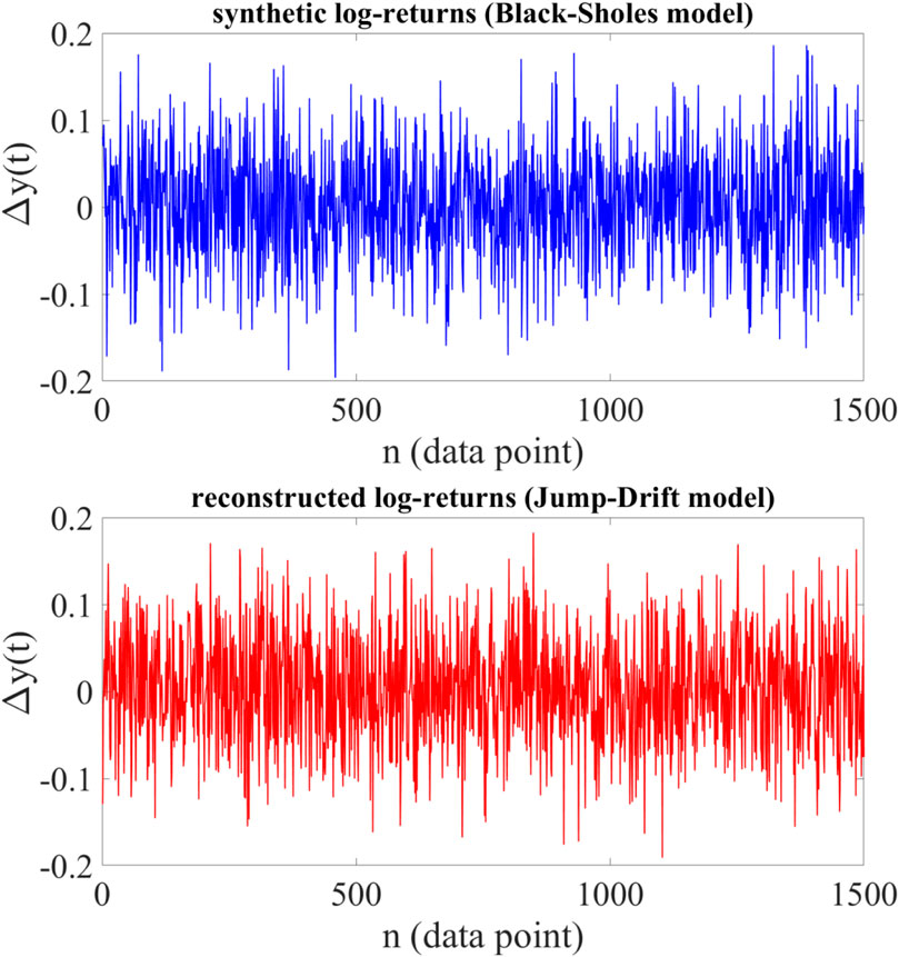
Figure 1. Upper panel: A sample path of synthetic log-returns generated via Black-Scholes dynamics using the preset parameters $\mu =1.5$, $\sigma =1$ and $∆t=0.004$. Lower panel: A sample path of log-returns reconstructed via jump-drift dynamics.

Statistical moments determined from generated data:

$M_1=0.004,M_2=0.004,M_4=4.8121\ast {10}^{-5},\frac{M_4}{3M_2^2}=1.002$

Required parameters for new modeling:

$\overline{\mu }=\frac{1}{∆t}{M}_1=1$

${\sigma }_{\xi }^2=\frac{M_4}{3M_2}=0.00401\left(\text{In\hspace{0.17em}agreement\hspace{0.17em}with\hspace{0.17em}}{\sigma }^2∆t=0.004\right)$

$\lambda ∆t=\frac{M_2}{{\sigma }_{\xi }^2}=0.997\approx 1$

In the second step, we reconstruct a time series $∆y\left(t\right)$ via the jump-drift equation (Eq. 16) with ${10}^6$ data points. For comparison with the original data, a sample path including 1,500 reconstructed data points is shown in Figure 1 (red graph). Finally, to ensure that the two time series (generated and reconstructed) are statistically equivalent, we obtain the statistical moments of the reconstructed data, and check the establishment of ${\left(\frac{M_4}{3M_2^2}\right)}_{rec}\approx 1$. The results are as follows:

Statistical moments of reconstructed data:

$M_1=0.004,M_2=0.004,M_4=4.8172*{10}^{-5},{\left(\frac{M_4}{3M_2^2}\right)}_{rec}=0.9985\approx 1$

As can be seen, the reconstructed data are statistically similar to original data with high accuracy, and there is a very good agreement between these results and the theory.

2.2 Jump-jump-drift modeling

In the previous section we modeled a continuous diffusion process through the jump-drift equation. Since real markets are usually jump-diffusion markets, the generalizing of jump-drift modeling to a jump-jump-drift modeling improves the characterization of real markets dynamics beyond a continuous process. The general form of a jump-jump-drift equation is as follows:

$dy\left(t\right)=\overline{\mu }dt+{\xi }_{1}d{J}_1\left(t\right)+{\xi }_{2}d{J}_2\left(t\right)(19)$

where $\overline{\mu }dt$ indicates the deterministic part of the process and $J_1\left(t\right)$ and $J_2\left(t\right)$ are Poisson jump processes. The jumps have rates ${\lambda }_1$ and ${\lambda }_2$, and sizes ${\xi }_1$ and ${\xi }_2$, which we assume have zero mean Gaussian distributions, i.e., ${\xi }_1\sim N\left(0,{\sigma }_{\xi 1}^2\right)$ and ${\xi }_2\sim N\left(0,{\sigma }_{\xi 2}^2\right)$. We call ${\sigma }_{\xi 1}^2$ and ${\sigma }_{\xi 2}^2$ the jump amplitudes.

Integration of Eq. 19 over ($t$, $t+∆t$) gives us:

$∆y\left(t\right)=\overline{\mu }∆t+{\xi }_1∆J_1\left(t\right)+{\xi }_2∆J_2\left(t\right)(20)$

Furthermore, the stock price can be determined from Eq. 20 as:

$S\left(t+∆t\right)=S\left(t\right)e^{\left(\overline{\mu }∆t+{\xi }_1∆J_1\left(t\right)+{\xi }_2∆J_2\left(t\right)\right)}(21)$

In modeling the stock price via Eq. 21, we also assume that two jumps do not occur simultaneously, which means that in the time interval $\left(t,t+∆t\right]$, if, for example, $∆J_1\left(t\right)$ occurs and takes the value of 1, $∆J_2\left(t\right)$ does not occur and its value is 0, and vice versa. Let ${\lambda }_1∆t$ and ${\lambda }_2∆t$ be the probabilities of occurrence of $∆J_1\left(t\right)$ and $∆J_2\left(t\right)$ in a small time step $∆t$, if we assume only one of the jumps ($∆J_1\left(t\right)$ or $∆J_2\left(t\right)$) occurs in each time step, then we can write:

${\lambda }_1∆t+{\lambda }_2∆t=1(22)$

According to this condition, we can discard one of the jump events at each time step, and reconstruct the corresponding data point by another jump event.

To model the stock prices via Eq. 20, we must find the five unknown parameters $\overline{\mu }$, ${\mathrm{\lambda }}_1∆t$, ${\mathrm{\lambda }}_2∆t$, ${\sigma }_{\xi 1}^2$ and ${\sigma }_{\xi 2}^2$. We now show that all these parameters can be estimated directly from the log-returns time series $∆y\left(t\right)$. For this purpose, we derive the statistical moments of $∆y\left(t\right)$ from Eq. 20 (note that ${\xi }_1$ and ${\xi }_2$ are two Gaussian random variables independent from the jumps, and $∆J_1\left(t\right)$ and $∆J_2\left(t\right)$ do not occur simultaneously):

$M_1=<∆y\left(t\right)>=<\overline{\mu }∆t>+<{\xi }_1><∆J_1\left(t\right)>+<{\xi }_2><∆J_2\left(t\right)>$

$M_2=<{\left(∆y\left(t\right)-\overline{\mu }∆t\right)}^2>=<{{\xi }_1}^2><{\left(∆J_1\left(t\right)\right)}^2>+{<{\xi }_2}^2><\left({\left(∆J_2\left(t\right)\right)}^2\right)>$

$M_4=<{\left(∆y\left(t\right)-\overline{\mu }∆t\right)}^4>=<{{\xi }_1}^4><{\left(∆J_1\left(t\right)\right)}^4>+<{{\xi }_2}^4><\left({\left(∆J_2\left(t\right)\right)}^4\right)>$

$M_6=<{\left(∆y\left(t\right)-\overline{\mu }∆t\right)}^6>=<{{\xi }_1}^6><{\left(∆J_1\left(t\right)\right)}^6>+<{{\xi }_2}^6><\left({\left(∆J_2\left(t\right)\right)}^6\right)>$

By using the relations $<{\left(∆J_1\left(t\right)\right)}^m>={\lambda }_1∆t$ and $<{\left(∆J_2\left(t\right)\right)}^m>={\lambda }_2∆t$ for the statistical moments of jump processes, and the relations $<{\xi }_1^{2l}>=\frac{2l!}{2^{l}l!}<{\xi }_1^2{>}^l$ and $<{\xi }_2^{2l}>=\frac{2l!}{2^{l}l!}<{\xi }_2^2{>}^l$ for the even order statistical moments of zero mean Gaussian random variables ${\xi }_1$ and ${\xi }_2$ with variances ${\sigma }_{{\xi }_1}^2$ and ${\sigma }_{{\xi }_2}^2$, we will have (note that $<{\xi }_1>=<{\xi }_2>=0$, $<{\xi }_1^2>={\sigma }_{{\xi }_1}^2$, and $<{\xi }_2^2>={\sigma }_{{\xi }_2}^2$):

$M_1=\overline{\mu }∆t$

$M_2={\sigma }_{{\xi }_1}^2{\lambda }_1∆t+{\sigma }_{{\xi }_2}^2{\lambda }_2∆t$

$M_4=3{\sigma }_{{\xi }_1}^4{\lambda }_1∆t+3{\sigma }_{{\xi }_2}^4{\lambda }_2∆t$

$M_6=15{\sigma }_{{\xi }_1}^6{\lambda }_1∆t+15{\sigma }_{{\xi }_2}^6{\lambda }_2∆t$

To find the five unknowns $\overline{\mu }$, ${\mathrm{\lambda }}_1∆t$, ${\mathrm{\lambda }}_2∆t$, ${\sigma }_{\xi 1}^2$ and ${\sigma }_{\xi 2}^2$, we need to add one more equation to the above relations. For this purpose, we use Eq. 22 as ${\lambda }_1∆t=1-{\lambda }_2∆t$, and reduce the number of unknowns, so we will have:

$M_1=\overline{\mu }∆t$

$M_2={\sigma }_{{\xi }_1}^2+\left({\sigma }_{{\xi }_2}^2-{\sigma }_{{\xi }_1}^2\right){\lambda }_2∆t$

$M_4=3{\sigma }_{{\xi }_1}^4+3\left({\sigma }_{{\xi }_2}^4-{\sigma }_{{\xi }_1}^4\right){\lambda }_2∆t$

$M_6=15{\sigma }_{{\xi }_1}^6+15\left({\sigma }_{{\xi }_2}^6-{\sigma }_{{\xi }_1}^6\right){\lambda }_2∆t(23)$

Having the statistical moments $M_1,M_2,M_4$ and $M_6$ from the log-return time series and solving the above system of equations numerically, the four unknown parameters $\overline{\mu }$, ${\mathrm{\lambda }}_2∆t$, ${\sigma }_{\xi 1}^2$ and ${\sigma }_{\xi 2}^2$ are determined. Once ${\mathrm{\lambda }}_2∆t$ is identified, ${\lambda }_1∆t$ is obtained from Eq. 22.

We claim that the proposed dynamics enables us to model time series with jump discontinuities more accurately than the classic jump-diffusion dynamics. We will check the validity of this claim by reconstructing a jump-diffusion process via the jump-jump-drift equation. But before that, let us prove this claim by showing that the new relations in Eq. 23 are generalizations of the old jump-diffusion relations in Eq. 11. For this purpose, we consider the case in which ${\sigma }_{{\xi }_1}^2\ll {\sigma }_{{\xi }_2}^2$, so that ${\sigma }_{{\xi }_1}^2$ can be ignored compared to ${\sigma }_{{\xi }_2}^2$, and at the same time ${\sigma }_{{\xi }_1}^2$ be so small that ${\sigma }_{{\xi }_1}^4={\sigma }_{{\xi }_1}^6=0$. Under these special conditions, relations (23) can be written as follows:

$M_1=\overline{\mu }∆t$

$M_2={\sigma }_{{\xi }_1}^2+{\sigma }_{{\xi }_2}^2{\lambda }_2∆t$

$M_4=3{\sigma }_{{\xi }_2}^4{\lambda }_2∆t$

$M_6=15{\sigma }_{{\xi }_2}^6{\lambda }_2∆t$

As can be seen, these relations are similar to relations of jump-diffusion model (Eq. 11), so that ${\sigma }_{{\xi }_1}^2$ has replaced ${\sigma }^2∆t$, and identifies the diffusion part, and ${\sigma }_{{\xi }_2}^2{\lambda }_2∆t$ has the same role as ${\sigma }_{\xi }^2\lambda ∆t$. This means that under these special conditions $\left({\sigma }_{{\xi }_1}^2\ll {\sigma }_{{\xi }_2}^2\right.$ and ${\sigma }_{{\xi }_1}^4={\sigma }_{{\xi }_1}^6=0$), the new model works like the jump-diffusion model and the parameters obtained from the data are the same in both models. But if the data fluctuations are such that these conditions are not satisfied, it is clear that the proposed model will lead to more accurate estimates than the jump-diffusion model. By analyzing stock prices, we found that although the release of exciting news in the market causes sudden jumps in log-returns, the amplitude of these jumps is not so much larger than the amplitude of the fluctuations in normal days. Therefore, it seems that the new model has a better performance for modeling and forecasting prices.

In the following, to demonstrate the reliability of the new model, we test it on synthetic data. Furthermore, to ensure the effectiveness of the proposed approach in different conditions, we test the model with different synthetic data.

Example 2:. First, we test the model with data generated through the Black-Scholes process in Example 1. By obtaining the statistical moments $M_n$ for $n=1,2,4,6$ from the generated data, and replacing them in relations (23), we determine the parameters required for the new modeling via the numerical solution of the obtained system of equations. Since the data generated in example 1 are diffusive data, and we have already modeled it through the jump-drift equation, we expect the occurrence rate of one of the jumps to be zero when we model the same data through the jump-jump-drift equation. The following results, confirm our opinion:

$\overline{\mu }=1$

${\sigma }_{\xi 1}^2=0.004$

${\lambda }_1∆t=0.9999\approx 1$

${\sigma }_{\xi 2}^2=0.0007$

${\lambda }_2∆t=0.0001\approx 0$

The value of ${\lambda }_2∆t\approx 0$ show that when the time series belongs to the class of continuous diffusion processes (e.g., Black-Scholes process), the jump-jump-drift dynamics, models it by using only one jump process and completely omitting the second jump process. In the next step, we test the model on two synthetic log-return time series generated via jump-diffusion Equation 9 with preset parameters. Each time series contains $3\times {10}^6$ data points which generated by considering $\overline{\mu }=5$ and $\sigma =2$ with a sampling interval $∆t=0.0001$, so that ${\sigma }^2∆t=0.0004$. The jumps in both time series have the same jump rate $\lambda ∆t=0.3$ (jump rate per data point), but the amplitude of the jumps are ${\sigma }_{\xi }^2=0.1$ and ${\sigma }_{\xi }^2=0.001$, respectively. We deliberately choose these jump amplitudes with different orders of magnitude to observe the effect of their amplitude in retrieving the coefficients. Note that in the first case $\frac{{\sigma }_{\xi }^2}{{\sigma }^2∆t}=250$ and in the second case $\frac{{\sigma }_{\xi }^2}{{\sigma }^2∆t}=2.5$, that is, in the first case, the variance of diffusion part (${\sigma }^2∆t$) is negligible compared to the amplitude of jumps (${\sigma }_{\xi }^2$), and as mentioned earlier, we expect both models show almost the same results, but in the second case, we expect the estimates of the new model to be more accurate than the jump-diffusion model.

By obtaining the statistical moments $M_n$ for $n=1,2,4,6$ from the generated data, and substituting in relations (11) and (23), we determine the parameters of the two models. The following results are estimated from the numerical solution of the corresponding system of equations:

Case1:. Preset parameters:

$\overline{\mu }=1,{\sigma }^2∆t=0.0004,{\sigma }_{\xi }^2=0.1,\lambda ∆t=0.3$

Estimated parameters via jump-diffusion model:

$\overline{\mu }=1,{\sigma }^2∆t=0.00031,{\sigma }_{\xi }^2=0.1005,\lambda ∆t=0.299$

Estimated parameters via jump-jump-drift model:

$\overline{\mu }=1,{\sigma }_{{\xi }_1}^2=0.00045,{\sigma }_{{\xi }_2}^2=0.1005,{\lambda }_2∆t=0.299,{\lambda }_1∆t=0.701$

Case2:. Preset parameters:

$\overline{\mu }=1,{\sigma }^2∆t=0.0004,{\sigma }_{\xi }^2=0.001,\lambda ∆t=0.3$

Estimated parameters via jump-diffusion model:

$\overline{\mu }=1,{\sigma }^2∆t=0.00013,{\sigma }_{\xi }^2=0.0012,\lambda ∆t=0.5$

Estimated parameters via jump-jump-drift model:

$\overline{\mu }=1,{\sigma }_{{\xi }_1}^2=0.00040,{\sigma }_{{\xi }_2}^2=0.0014,{\lambda }_2∆t=0.302,{\lambda }_1∆t=0.698$

The above results show that in the first case, both models lead to almost the same results, but in the second case, the proposed model leads to more accurate results (note that in the new model, ${\sigma }_{{\xi }_1}^2$ is an estimate for the variance of the diffusive data, i.e., ${\sigma }_{{\xi }_1}^2={\sigma }^2∆t$, and ${\sigma }_{{\xi }_2}^2$ is an estimate for the variance of the jumpy data, i.e., ${\sigma }_{{\xi }_2}^2={\sigma }_{\xi }^2$).

3 Data and methodology

Our dataset comprises the daily closing prices of the Apple and IBM stocks, as well as gold prices with two different time horizons (weekly and hourly). For Apple and IBM stocks, the historical data that will be used are daily closing prices from 1 June 2020 to 1 June 2023, which are obtained from Yahoo Finance source. For gold, the historical data that will be used are weekly gold prices from 5 January 2004 to 3 January 2022, as well as hourly gold prices from 11 March 2022 to 11 November 2022, which are obtained from dukascopy historical data source.

For each of the collected data, we will obtain log-returns time series $∆y\left(t\right)$ by:

$∆y\left(t\right)=\ln \left[\frac{S\left(t+∆t\right)}{S\left(t\right)}\right],t=1,2,\dots \dots$

where $S\left(t\right)$ and $S\left(t+1\right)$ are consecutive prices in the price time series. Afterwards, we will determine the statistical moments of log-returns data as follows:

$M_1=\overline{∆y}=\frac{1}{N}{\displaystyle \sum _{t=1}^N}∆y\left(t\right)$

$M_n=\frac{1}{N}{\displaystyle {\sum }_{t=1}^N}(∆y\left(t\right)-\overline{∆y}{)}^n,\text{for\hspace{0.17em}}n=2,4,6$

where $N$ is the number of log-returns data points. By determining these statistical moments and replacing them in relations (23), we will identify the required parameters of the model, i.e., $\overline{\mu }$, ${\sigma }_{\xi 1}^2$, ${\sigma }_{\xi 2}^2$, ${\lambda }_1∆t$, ${\mathrm{\lambda }}_2∆t$. Using these parameters, we will reconstruct the log-returns data by the following equation:

$∆y\left(t\right)=\overline{\mu }∆t+{\xi }_1∆J_1\left(t\right)+{\xi }_2∆J_2\left(t\right)$

In addition, we will use the following equation to forecast prices for several time steps after the chosen historical period:

$S\left(t+1\right)=S\left(t\right)e^{\left(\overline{\mu }∆t+{\xi }_1∆J_1\left(t\right)+{\xi }_2∆J_2\left(t\right)\right)}$

To determine the forecasts accuracy, we will use “Mean Absolute Percentage Error” (MAPE) calculation as follows:

$\text{MAPE}=\frac{1}{N}{\displaystyle {\sum }_{t=1}^N}\frac{\left|F\left(t\right)-S\left(t\right)\right|}{S\left(t\right)}$

where $F\left(t\right)$ is the forecasted price at time $t$, $S\left(t\right)$ is the actual stock price at time $t$, and $N$ is the number of predicted data points. We will use MAPE values to evaluate our forecasting method. A scale for judging model accuracy based on the MAPE criterion was presented by Lawrence et al. [23], and is shown in Table 1.

Table 1

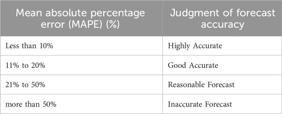
Table 1. A scale of judgment of forecast accuracy.

3.1 Research output and discussion

In the following, considering the elements described in the methodology, we first model Apple and IBM stocks and predict their prices for a period of 30 days. Historical data used are daily closing stock prices from 1 June 2020 to 1 June 2023. For daily prices, the trading period is $∆t=\frac{1}{252}$ years (based on a year with an average of 252 stock trading days). The parameters obtained from the model are presented in Table 2. Based on this table, in both stocks, ${\sigma }_{{\xi }_2}^2$ is not more than one order of magnitude larger than ${\sigma }_{{\xi }_1}^2$, so that for Apple stock we have $\frac{{\sigma }_{{\xi }_2}^2}{{\sigma }_{{\xi }_1}^2}=4.34$, and for IBM stock this ratio is $\frac{{\sigma }_{{\xi }_2}^2}{{\sigma }_{{\xi }_1}^2}=4.2$. As mentioned earlier, in this situation, the new model has better performance. Furthermore, for the Apple stock, the jump rates are ${\lambda }_1∆t=0.8248$ and ${\lambda }_2∆t=0.1752$, which means that, in the data reconstruction stage, 82.48% of the data points are reconstructed by using a Gaussian random variable with smaller variance ${\sigma }_{{\xi }_1}^2$, and 17/52% of the data points are reconstructed by using a Gaussian random variable with larger variance ${\sigma }_{{\xi }_2}^2$. This is while, these rates for the IBM stock are ${\lambda }_1∆t=0.6790$ and ${\lambda }_2∆t=0.3210$, respectively.

Table 2

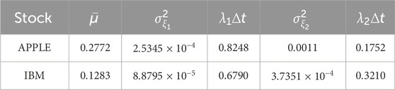
Table 2. values of the drift, jump amplitudes, and jump rates obtained from historical daily prices of Apple and IBM stocks using the jump-jump-drift modeling.

To reconstruct log-return data through proposed model, we use the equation $∆y\left(t\right)=\overline{\mu }∆t+{\xi }_1∆J_1\left(t\right)+{\xi }_2∆J_2\left(t\right)$ and reconstruct a time series for $∆y\left(t\right)$ that is statistically similar to the original ones. Figures 2, 3 show the actual and reconstructed log-returns of Apple and IBM stocks, respectively.

Figure 2

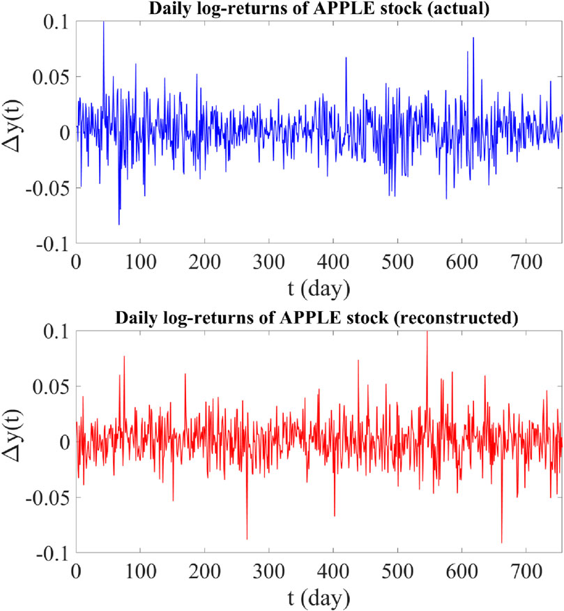
Figure 2. Upper panel: Time plot of actual daily log-returns of Apple stock from 1 June 2020 to 1 June 2023 (756 data points). Lower panel: Time plot of reconstructed daily log-returns of Apple stock using the proposed jump-jump-drift model.

Figure 3

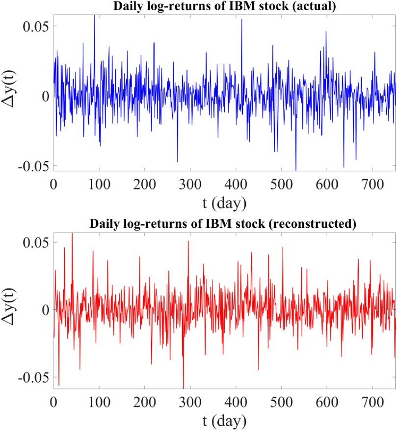
Figure 3. Upper panel: Time plot of actual daily log-returns of IBM stock from 1 June 2020 to 1 June 2023 (756 data points). Lower panel: Time plot of reconstructed daily log-returns of IBM stock using the proposed jump-jump-drift model.

To predict stock prices, we use parameters estimated from historical data. The forecast period is 30 days and is related to the days after the selected historical period. Simulation of predictions is done by 1,000 realization of the trajectory. Each trajectory is realized using the equation $S\left(t+1\right)=S\left(t\right)e^{\left(\overline{\mu }∆t+{\xi }_1∆J_1\left(t\right)+{\xi }_2∆J_2\left(t\right)\right)}$ with 30 iterations. Figures 4, 5 show the daily forecasts of Apple and IBM stock prices, respectively. In order to compare the predictions with the actual prices, the graph of realized prices in the same 30 days is also shown in each figure (cyan graph). As can be seen, in both stocks, the actual prices are located within the predicted trajectories. In addition, the data analysis shows that all 1,000 predicted trajectories of Apple stock price have MAPE values less than 20% (with the smallest MAPE = 1.4%, the largest MAPE = 19.8% and the average MAPE = 5.84%). Meanwhile, the corresponding values obtained through the jump-diffusion model are as follows:

Figure 4

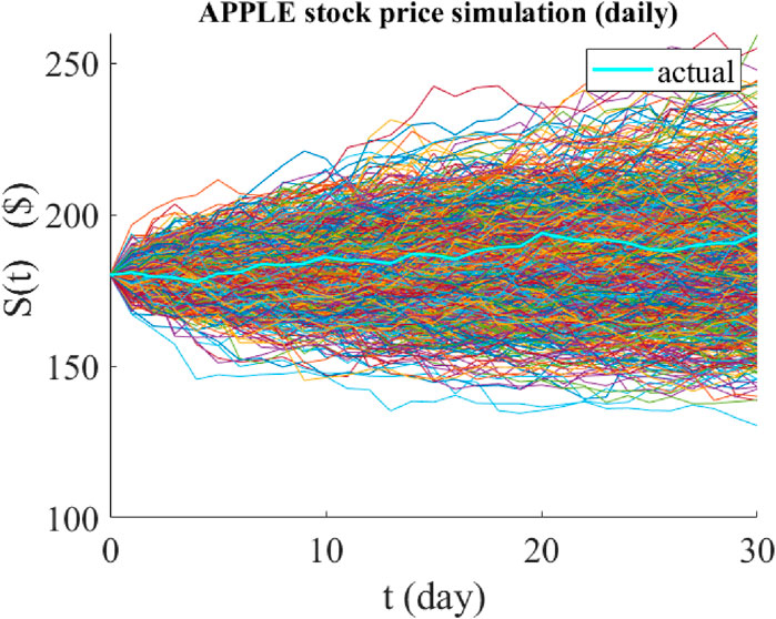
Figure 4. Graphical representation of the predicted paths of the daily price of Apple stock using jump-jump-drift modeling. The time period of all predictions is 30 days and their starting point is 1 June 2023. The cyan graph is the actual price path realized over the same 30 days, and the colored graphs are the 1,000 possible paths predicted by the model.

Figure 5

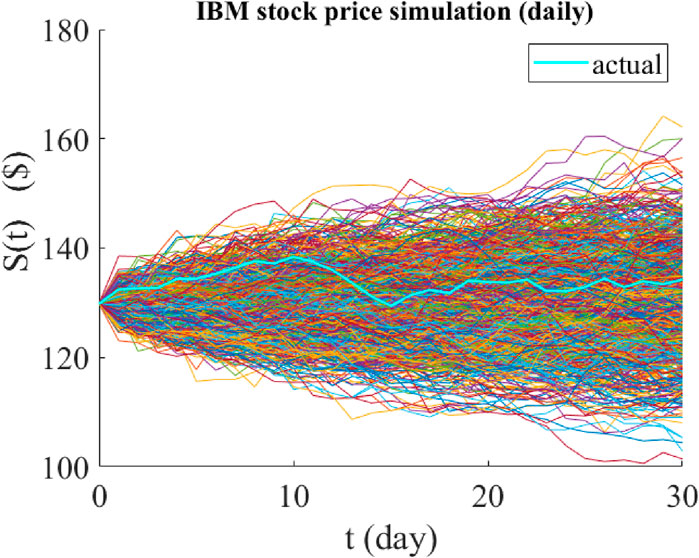
Figure 5. Graphical representation of the predicted paths of the daily price of IBM stock using jump-jump-drift modeling. The time period of all predictions is 30 days and their starting point is 1 June 2023. The cyan graph is the actual price path realized over the same 30 days, and the colored graphs are the 1,000 possible paths predicted by the model.

The smallest MAPE = 1.51%, the largest MAPE = 24.3%, and the average MAPE = 6.32%. These results show that the jump-jump-drift model has a better performance than the jump-diffusion model, and if the time period of the forecasts becomes larger (e.g., in annual forecasts), the difference between the forecasts of the two models becomes more visible.

The results of IBM stock price predictions are even more surprising than Apple stock. Analysis of IBM stock simulation outputs shows that all 1,000 predicted trajectories have MAPE values ​​less than 15% (with the smallest MAPE = 1.22%, the largest MAPE = 14.02% and the average MAPE = 4.62%), indicating good accuracy of the model predictions. The corresponding values obtained through jump-diffusion model are as follows:

The smallest MAPE = 1.62%, the largest MAPE = 20.7%, and the average MAPE = 5.12%.

Finally, to see the effectiveness of the proposed approach for different time horizons, we simulate gold prices with two different time horizons. Historical data used are weekly gold price from 5 January 2004 to 3 January 2022, as well as hourly gold prices from 11 March 2022 to 11 November 2022. For weekly prices, the trading period is $∆t=\frac{1}{52}$ years (based on a year with an average of 52 trading weeks), while for hourly prices, the trading period is $∆t=\frac{1}{5916}$ years (based on 2022 with 5,916 trading hours). The parameters obtained from the model are presented in Table 3. Based on this table, in both cases, ${\sigma }_{{\xi }_2}^2$ is not more than one order of magnitude larger than ${\sigma }_{{\xi }_1}^2$, so that for weekly data we have $\frac{{\sigma }_{{\xi }_2}^2}{{\sigma }_{{\xi }_1}^2}=4.6$, and for hourly data this ratio is $\frac{{\sigma }_{{\xi }_2}^2}{{\sigma }_{{\xi }_1}^2}=11.7$.

Table 3

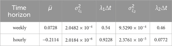
Table 3. values of the drift, jump amplitudes, and jump rates obtained from historical gold prices (weekly and hourly) using jump-jump-drift modeling.

To reconstruct log-return data through proposed model, we use the equation $∆y\left(t\right)=\overline{\mu }∆t+{\xi }_1∆J_1\left(t\right)+{\xi }_2∆J_2\left(t\right)$ and reconstruct a time series for $∆y\left(t\right)$ that is statistically similar to the original ones. Figures 6, 7 show the actual and reconstructed log-returns of weekly and hourly prices of gold, respectively.

Figure 6

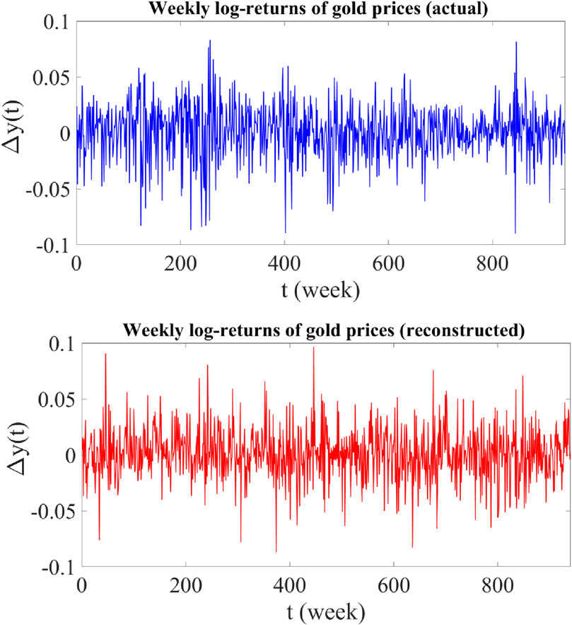
Figure 6. Upper panel: Time plot of actual weekly log-returns of gold prices from 5 January 2004 to 3 January 2022 (940 data points). Lower panel: Time plot of reconstructed weekly log-returns of gold prices using the proposed jump-jump-drift model.

Figure 7

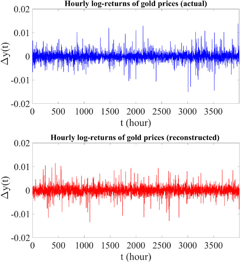
Figure 7. Upper panel: Time plot of actual hourly log-returns of gold prices from 11 March 2022 to 11 November 2022 (3,999 data points). Lower panel: Time plot of reconstructed hourly log-returns of gold prices using the proposed jump-jump-drift model.

To predict gold prices, we use parameters estimated from historical data. The forecast period for weekly price is 30 weeks and for hourly price is 300 h and related to the times after historical periods. Simulation of predictions is done by 1,000 realization of the trajectory. Each trajectory is realized using the equation $S\left(t+1\right)=S\left(t\right)e^{\left(\overline{\mu }∆t+{\xi }_1∆J_1\left(t\right)+{\xi }_2∆J_2\left(t\right)\right)}$ with 30 iterations for weekly gold price and 300 iterations for hourly gold price. Figures 8, 9 show the weekly and hourly gold price forecasts, respectively. As can be seen, in both cases, the actual prices are located within the trajectories predicted by the model. Furthermore, the data analysis shows that all 1,000 predicted trajectories of weekly gold price have MAPE values ​​less than 30% (with the smallest MAPE = 2.1%, the largest MAPE = 29.43% and the average MAPE = 7.57%), which are acceptable forecasts. The corresponding values obtained by jump-diffusion model are as follows:

Figure 8

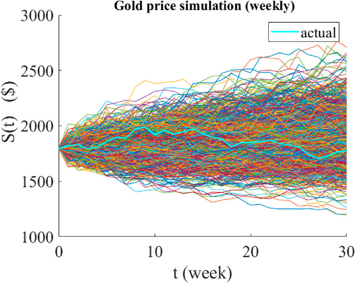
Figure 8. Graphical representation of the predicted paths of the weekly price of gold using jump-jump-drift modeling. The time period of all predictions is 30 weeks and their starting point is 3 January 2022. The cyan graph is the actual price path realized over the same 30 weeks, and the colored graphs are the 1,000 possible paths predicted by the model.

Figure 9

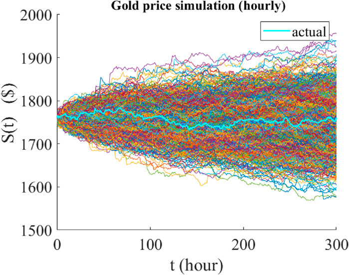
Figure 9. Graphical representation of the predicted paths of the hourly price of gold using jump-jump-drift modeling. The time period of all predictions is 300 h and their starting point is 11 November 2022. The cyan graph is the actual price path realized over the same 300 h, and the colored graphs are the 1,000 possible paths predicted by the model.

The smallest MAPE = 2.3%, the largest MPAE = 35.7%, and the average MAPE = 7.85%.

Analysis of hourly gold prices shows that all 1,000 predicted paths have MAPE values ​​less than 10% (with the smallest MAPE = 0.51%, the largest MPAE = 7.17% and the average MAPE = 1.82%), indicating very high accuracy of the model predictions for hourly time horizons. The corresponding values obtained by jump-diffusion model are as follows:

The smallest MAPE = 0.8%, the largest MPAE = 10.3%, and the average MAPE = 2.15%.

4 Conclusion

We discussed that when data are sampled at discrete times (e.g., stock prices), they appear as a sequence of discontinuous jump events, even if they have been sampled from a continuous process. This issue gave us the idea to propose a new modeling in which random variations in the sample path of a measured time series are attributed to jump events, even if the time series belongs to the class of diffusion processes. Based on this, we introduced a new dynamical stochastic equation including a deterministic drift term and a combination of several stochastic terms with jumpy behaviors. The general form of this equation is as follows:

$dy\left(t\right)=\overline{\mu }dt+{\displaystyle \sum _{i=1}^N}{\xi }_{i}d{J}_i\left(t\right)$

In this modeling we also assumed that the jump events do not occur simultaneously so that the jumps have no overlap. We started with the simplest form of equation including a deterministic drift term and a jump process as the stochastic component, and argued that it can be used to describe the discrete-time evolution of a diffusion process, e.g., Black-Scholes process. Afterwards, we extended the equation by considering two jump processes with different distributed sizes, and used it to model assets such as stock prices and gold prices with different time horizons. We also demonstrated that in all cases the proposed model works better than the old jump model. It should be noted that, due to the small number of available price data and the lack of diversity in the amplitudes of jumps, in this article we modeled prices data only by considering two jump processes. However, depending on the number of data points and variation in the amplitudes of fluctuations, more stochastic terms can be kept in the equation to increase the accuracy of the modeling. But on the other hand, the more the number of terms in the equation, the need to solve the system of equations with more unknowns, the cost of which must be paid in the form of longer runtime.

Data availability statement

The original contributions presented in the study are included in the article/Supplementary Material, further inquiries can be directed to the corresponding author.

Author contributions

AM: Conceptualization, Data curation, Formal Analysis, Funding acquisition, Investigation, Methodology, Project administration, Resources, Software, Supervision, Validation, Visualization, Writing–original draft, Writing–review and editing. HN: Conceptualization, Data curation, Formal Analysis, Funding acquisition, Investigation, Methodology, Project administration, Resources, Software, Supervision, Validation, Visualization, Writing–original draft, Writing–review and editing.

Funding

The author(s) declare that no financial support was received for the research, authorship, and/or publication of this article.

Conflict of interest

The authors declare that the research was conducted in the absence of any commercial or financial relationships that could be construed as a potential conflict of interest.

Publisher’s note

All claims expressed in this article are solely those of the authors and do not necessarily represent those of their affiliated organizations, or those of the publisher, the editors and the reviewers. Any product that may be evaluated in this article, or claim that may be made by its manufacturer, is not guaranteed or endorsed by the publisher.

References

1. Reddy K, Clinton V. Simulating stock prices using geometric Brownian motion: evidence from Australian companies. Australas Account Business Finance J (2016) 10(3):23–47. doi:10.14453/aabfj.v10i3.3

CrossRef Full Text | Google Scholar

2. Synowiec D. Jump-diffusion models with constant parameters for financial log-return processes. Comput Math Appl (2008) 56(8):2120–7. doi:10.1016/j.camwa.2008.02.051

CrossRef Full Text | Google Scholar

3. Azizah M, Irawan M, Putri E. Comparison of stock price prediction using geometric Brownian motion and multilayer perceptron. In: AIP conference proceedings: Depok, Indonesia. AIP Publishing (2020).

CrossRef Full Text | Google Scholar

4. Mota PP, Esquível ML. Model selection for stock prices data. J Appl Stat (2016) 43(16):2977–87. doi:10.1080/02664763.2016.1155205

CrossRef Full Text | Google Scholar

5. Benninga S. Financial modeling, fourth edition By Simon Benninga Hardcover. The MIT press (2014).

Google Scholar

6. Bachelier L. Théorie de la spéculation. In: Annales scientifiques de l’École normale supérieure (1900).

CrossRef Full Text | Google Scholar

7. Osborne MF. Brownian motion in the stock market. Operations Res (1959) 7(2):145–73. doi:10.1287/opre.7.2.145

CrossRef Full Text | Google Scholar

8. Samuelson PA. Economic theory and mathematics--an appraisal. Am Econ Rev (1952) 42(2):56–66.

Google Scholar

9. Black F, Scholes M. The pricing of options and corporate liabilities. J Polit economy (1973) 81(3):637–54. doi:10.1086/260062

CrossRef Full Text | Google Scholar

10. Black F, Karasinski P. Bond and option pricing when short rates are lognormal. Financial Analysts J (1991) 47(4):52–9. doi:10.2469/faj.v47.n4.52

CrossRef Full Text | Google Scholar

11. Risken H. Springer series in synergetics (1996).

Google Scholar

12. Bouchaud J-P, Cont R. A Langevin approach to stock market fluctuations and crashes. Eur Phys J B-Condensed Matter Complex Syst (1998) 6:543–50. doi:10.1007/s100510050582

CrossRef Full Text | Google Scholar

13. Hull J, White A. The pricing of options on assets with stochastic volatilities. J Finance (1987) 42(2):281–300. doi:10.1111/j.1540-6261.1987.tb02568.x

CrossRef Full Text | Google Scholar

14. Mercurio D, Spokoiny V. Estimation of time dependent volatility via local change point analysis (2005).

Google Scholar

15. Goldentayer L, Klebaner F, Liptser RS. Tracking volatility. Probl Inf Transm (2005) 41:212–29. doi:10.1007/s11122-005-0026-2

CrossRef Full Text | Google Scholar

16. Merton RC. Option pricing when underlying stock returns are discontinuous. J financial Econ (1976) 3(1-2):125–44. doi:10.1016/0304-405x(76)90022-2

CrossRef Full Text | Google Scholar

17. Heston SL. A closed-form solution for options with stochastic volatility with applications to bond and currency options. Rev financial Stud (1993) 6(2):327–43. doi:10.1093/rfs/6.2.327

CrossRef Full Text | Google Scholar

18. Nelson DB. ARCH models as diffusion approximations. J Econom (1990) 45(1-2):7–38. doi:10.1016/0304-4076(90)90092-8

CrossRef Full Text | Google Scholar

19. Anvari M, Tabar MRR, Peinke J, Lehnertz K. Disentangling the stochastic behavior of complex time series. Scientific Rep (2016) 6(1):35435. doi:10.1038/srep35435

PubMed Abstract | CrossRef Full Text | Google Scholar

20. Tabar R. Analysis and data-based reconstruction of complex nonlinear dynamical systems, 730. Springer (2019).

Google Scholar

21. Lehnertz K, Zabawa L, Tabar MRR. Characterizing abrupt transitions in stochastic dynamics. New J Phys (2018) 20(11):113043. doi:10.1088/1367-2630/aaf0d7

CrossRef Full Text | Google Scholar

22. Movahed AA, Noshad H. Introducing a new approach for modeling a given time series based on attributing any random variation to a jump event: jump-jump modeling. Scientific Rep (2024) 14(1):1234. doi:10.1038/s41598-024-51863-5

CrossRef Full Text | Google Scholar

23. Excel FOFU. Fundamentals of forecasting using excel (2019).

Google Scholar