 G. Martini
 E. Tentori
 M. Mirigliano
 D. E. Galli1*‡
 P. Milani
 F. Mambretti
- 1CIMAINA and Department of Physics, University of Milan, Milan, Italy
- 2Padova Neuroscience Center, Università degli Studi di Padova, Padova, Italy
- 3Dipartimento di Fisica e Astronomia, Università degli Studi di Padova, Padova, Italy
- 4Atomistic Simulations group, Italian Institute of Technology, Genova, Italy
Amid efforts to address energy consumption in modern computing systems, one promising approach takes advantage of random networks of non-linear nanoscale junctions formed by nanoparticles as substrates for neuromorphic computing. These networks exhibit emergent complexity and collective behaviors akin to biological neural networks, characterized by self-organization, redundancy, and non-linearity. Based on this foundation, a generalization of n-inputs devices has been proposed, where the associated weights depend on all the input values. This model, called receptron, has demonstrated its capability to generate Boolean functions as output, representing a significant breakthrough in unconventional computing methods. In this work, we characterize and present two actual implementations of this paradigm. One approach leverages the nanoscale properties of cluster-assembled Au films, while the other utilizes the recently introduced Stochastic Resistor Network (SRN) model. We first provide a concise overview of the electrical properties of these systems, emphasizing the insights gained from the SRN regarding the physical processes within real nanostructured gold films at a coarse-grained scale. Furthermore, we present evidence indicating the minimum complexity level required by the SRN model to achieve a stochastic dynamics adequate to effectively model a novel component for logic systems. To support our argument that these systems are preferable to conventional random search algorithms, we discuss quantitative criteria based on Information-theoretic tools. This suggests a practical means to steer the stochastic dynamics of the system in a controlled way, thus focusing its random exploration where it is most useful.
1 Introduction
The urgent need of a substantial improvement in environmental footprint, associated with the capability of performing complex tasks with ever-increasing amounts of data, has raised the interest on Unconventional Computing Systems (UCS) as a viable alternative to data processing based on CMOS technology and von Neumann architecture [1, 2]. One of the common traits of UCS is the exploitation of the complexity emerging from generic underlying physical substrates for computation. Among several approaches, we just recall molecular, optical, chemical and in materia computing [3–12]. To this end, a new paradigm recently emerged in this field is the receptron (reservoir perceptron), a generalization of perceptron [13, 14]. While perceptron’s weights associated with each input are independent and must be individually adjusted to give the desired output [15], in the receptron model a network of highly interconnected nonlinear objects adjusts its conduction pathway topology depending on the input stimuli, such that the weighting process is not just responding separately to each stimulus but is sensitive to their co-location. Network’s weights are, then, functions of a convolution of the spatial location of the input topology. Thus, a receptron can be used as a binary classification tool to map the inputs from different electrodes in two possible sets labeled by 0 and 1. If the inputs are also binary, the device can be employed as a Boolean function generator [16]. The potential of such a device resides in its capability to generate a complete set of Boolean functions (including those non-linearly separable) of n variables for classification tasks [17], without having been explicitly programmed for that. Practical realizations of the receptron include devices made of a nanostructured metallic film interconnecting a generic pattern of electrical contacts. In particular, a promising hardware implementation of the receptron is represented by cluster-assembled nanostructured Au films, which have recently been shown to have a complex resistive switching activity together with potentiation behavior [17–21]. Such devices, which have been extensively characterized experimentally, are here discussed - together with an abstract model of receptron - as a relevant example of this new computing paradigm. The internal nanostructure of these gold films is repeatedly altered by the application of input stimuli, and we anticipate that this property candidates such objects as suitable devices for computation.
The Boolean function generation is designed as a dynamic process, thanks to the possibility of a plastic rearrangement of the nanostructured conductive medium: the nanojunctions’ network that constitute the film can be reconfigured via the administration of stimuli of amplitude larger than a threshold voltage Vth, during the device reprogramming [20, 22, 23]. The specific modification of the conductive paths will then depend on the particular electrode configuration [17]. Subsequently, in the compute step, the sample resistance is probed via the application of sub-threshold voltage input signals, which do not alter the structure and topology of the conduction paths. Thanks to the extremely large number of conductive states available to the system, the device can be effectively used as a binary classifier: it behaves as a nonvolatile, reconfigurable function generator without any previous training [16]. The stochasticity of the output calls for the identification of a few hyperparameters of the experimental setup that can be tuned to improve the predictability of the Boolean outputs.
An abstract model known as Stochastic Resistor Network (SRN) enables a thorough examination of the electrical properties of this nanostructured system, via a large three-dimensional (3D) regular resistor network [18]. The conductance of a small portion of the film is represented as an edge in an abstract graph conceptualization. Each edge weight can evolve to a new discretized conduction value, according to stochastic local physical rules, shaping the collective dynamics of the system. Probabilistic updates are deduced from empirical effects, including local thermal dissipation and nonlinear conduction mechanisms. Going beyond one-to-one mapping of all the conductive junctions between gold nanoparticles, the SRN offers a coarse-grained representation of the intricate dynamics within the film’s internal structure. Integrating the network with very high conductive edges that act as electrodes readily provides an implementation of the receptron model. The system inherently exhibits diverse dynamic behaviors tailored to different magnitudes of external electrical stimulation.
Here we formally define the problem of characterizing and governing the receptron stochasticity, striving to gain improved performances, together with a detailed description of its implementation. With the insights provided by the SRN model, we assess the susceptibility to the parameters that regulate the main dynamical features of the receptron reprogramming dynamics. The comparison between the simulations and the experimental system suggests the constructive characteristics that are needed for a receptron to sample the Boolean function space with increased efficiency. Using tools derived from Information theory, we prove that, to some extent, the effectiveness of the receptron in generating Boolean functions can be boosted via specific reprogramming protocols.
2 Materials and methods
2.1 The receptron
The digital receptron [13] is a reprogrammable, nonlinear threshold logic gate. Digital inputs
where
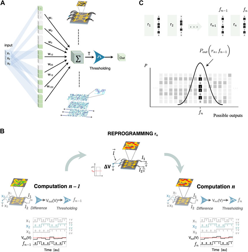
Figure 1. (A) Schematic representation of computation taking place in the receptron with three Boolean inputs (
While the additional possibilities offered by the nonlinearity have already been discussed elsewhere [13], little attention has been given to the reprogramming procedure itself, especially in relation to common experimental limits, like intrinsic long-term dynamics and sample-to-sample variability. The two experimental receptron implementations proposed so far, optical [13] and electrical [17], both rely on substrates for the weighting of the inputs, that cannot be reconfigured in a deterministic manner: such complex weighting media evolve according to a stochastic dynamics that cannot be completely captured by a set of differential equations. Here we focus on the electrical implementation [16] of a 3-bit (input) receptron to show how an intrinsically random reprogramming of a complex system can still be controlled and characterized to improve the performance of the computing device. Even if complete randomicity may only be an extreme case scenario, the results presented here can be used to deal with all systems whose complicated modeling prevents a controlled and precise tailoring of the internal state or where sample to sample variability exceeds the tolerance of such a mathematical description.
2.2 Experimental and simulated receptrons
As anticipated, in this work we make use of an experimental and an in silico implementation of an electrical receptron (see Eq. 1), each featuring a three-channel input. Both realizations exploit a central non-ohmic conducting medium for the weighting process: two electrical currents I1 and I2 flowing out such a complex network are subtracted to obtain an analog value which is then thresholded (performed at the software level). The internal set of weights is encoded as the resistive state of the experimental/simulated nanostructured network: these can be reprogrammed by triggering a resistive switching phenomenon, i.e., a plastic rearrangement of the resistive network through the delivery of high voltage pulses [17].
2.2.1 Experimental receptron implementation
In the experimental implementation of the receptron [17], a three-input configuration exploits the electrical behavior of a multi-electrode nanostructured Au film. The assembly of nanoscopic (mean size around 6 nm) clusters of gold atoms on a flat silicon-oxide substrate results in a defect-rich (mainly grain boundaries) film whose intricated conductive paths result from the interaction of several branched aggregates, which grow as thickness is increased until the formation of spanning aggregates when the percolation threshold is exceeded [20, 21, 24]. The significant decrease in electrical conductivity resulting from such a high number of defects is accompanied by a multitude of resistance states that can be reached by inducing rearrangements of the nanostructure. As local temperature increases due to joule heating, cluster aggregates can experience significant morphological changes leading to macroscopically different current pathways [22, 25].
The electrical setup (Figure 1B) consists of three relays on the left, connected to respective electrodes, enabling the switching between voltage supply and open circuit. Two relays, connected to the extremal output electrodes on the right, allow the switching between ground terminals, via a digital multimeter for current measurement, and open circuit. As for many memristive systems [27], the reprogramming and computation are both the result of electrical stimuli, which only differ in magnitude. When computing, a low voltage (
2.2.2 In-silico simulation of the receptron
The simulated network uses the SRN model [18], which involves a stochastic evolution of resistors to represent the distribution of conductive regions within a cluster-assembled gold film [17, 27]. Each link represents a coarse-grained portion of the percolating network which can assume one of four possible conductance levels: an insulating one or three distinct conductive ones. At each simulation step, every link can stochastically switch to another level using Monte Carlo (MC) moves (see Supplementary Material and Ref. [18]): these mimic local thermal dissipation near crystalline orientation mismatches and nonlinear phenomena across the band gap described for the experimental system [17, 20, 21, 28]. Briefly, each link conductance
After each MC move, Kirchoff’s equations are used to solve the network [29, 30]. Note that in our SRN complex physical phenomena arise from probabilistic update rules, which draw inspiration from microscopic-scale physics. This key aspect distinguishes our system’s evolution from other models that directly replicate potentiation mechanisms (see, e.g., [31]). The SRN shares some common features (the regular grid, the way the network is solved, the local Joule effect) with other models like the simpler Random Fuse Model (RFM) [32], which was nonetheless conceived to study only the breaking process of materials traversed by current. Conversely, the stochastic evolution of the SRN, the ability to reproduce more physical effects than just the breaking and reforming of connections [33] and the easy adaptability to mimic a real experimental setup constitute major differences with respect to the old RFM.
Here, the simulated network exploits three electrode-nodes (ENs) to establish connections between the source and the network through as many groups of permanent-conductive links (ELs). These ELs are strategically positioned to mimic three input electrodes and can be connected to the source node through three permanent switch-links (SLs). SLs serve as switches between ENs and the source, allowing different configurations. The network’s multi-channel setup, together with its 3D structure, is represented in Supplementary Figure S1, which also features two output electrodes for connection to the ground. At each simulation step, it is consistently feasible to measure the resistance of every network component and the current passing through each edge, particularly the current exiting the network during computation (as illustrated in Figure 3A). This setup enables the simulation of computation and reprogramming phases, both of which adhere to the same logic as the experimental implementation of the receptron (see Supplementary Material for the definition of the threshold voltage Vth in the simulated case).
Note that our analyses benefit from the regularity of the network, which has a simpler geometry if compared with recently introduced models for nanowire networks [34]. Such models feature a much more complex organization of the nodes and links, but we do believe that this choice would not modify our findings since those are not related in any way to the peculiar adjacency matrix of the simulated network.
2.3 Receptron reprogramming
The experimental and simulated receptron reprogramming is the result of current flow during the application of high voltage stimuli. Here we identify a series of control parameters that, by shaping the distribution of electrical currents, are instrumental in influencing the evolution of the physical system and, consequently, the dynamics of the weights. Overall, the effect of reprogramming is determined by the complex interplay of the voltage stimulus magnitude, polarity, and localization (that is, the boundary conditions that constrain the current flow). We will refer to these parameters with
Being ∆V ∈ [
As a first order approximation, we assume that the state transition process is Markovian [35]: this ansatz is validated by the decay of the autocorrelation function for the output (see Supplementary Material) which has a characteristic low correlation step, between 1 and 4. Given this assumption, the output function
as schematically represented in Figure 1C.
We will determine which parameters contained in
2.4 Calculating mutual information between reprogramming parameters and receptron outputs
The goal of identifying the most effective reprogramming hyper-parameters can be achieved by a specific reprogramming protocol, wherein alternating cycles of reprogramming and output computation are conducted.
We quantify the receptron susceptibility to diverse reprogramming protocols by computing the Mutual Information between the reprogramming sequence R and output functions sequence F, MI (
quantifies the amount of reduction in uncertainty about the output given knowledge of the input [36], and a significantly non-vanishing ratio of MI(R,F)/H(F) would imply that it is possible to extract relevant information about the output based on the chosen reprogramming scheme. This approach allows for efficient characterization of the device’s functioning, as it avoids the need for extensive grid-search experiments that could be difficult to perform on a statistically significant batch of devices, due to inter-device variability.
In our study, we want to verify that the following is significantly true:
To compute the entropies, we have used the natural logarithm and applied the correction term proposed by [37]. This correction term is given by:
where “ ⋅ ” is a generic observable,
In experiments and analogously in simulations we have estimated pi using a frequentist approach. F is defined to be implemented output function represented as a decimal number, and it depends on the specific thresholding that is implemented, while H(
2.4.1 Significant Mutual Information test
Statistically dependent input and output sets are expected to have higher Mutual Information than would occur by chance. To determine the significance of the Mutual Information measured, we used a standard
3 Results
3.1 Internal dynamics of the Stochastic Resistor Network
SRN simulations offer an important perspective on what is happening to the complex network during reprogramming. In the forthcoming example, we explore the effect on the analog weighted output,
Figure 2 illustrates the relationship between the outputs and the network restructuring. Figure 2A presents an example (focusing on 110 MC steps) of
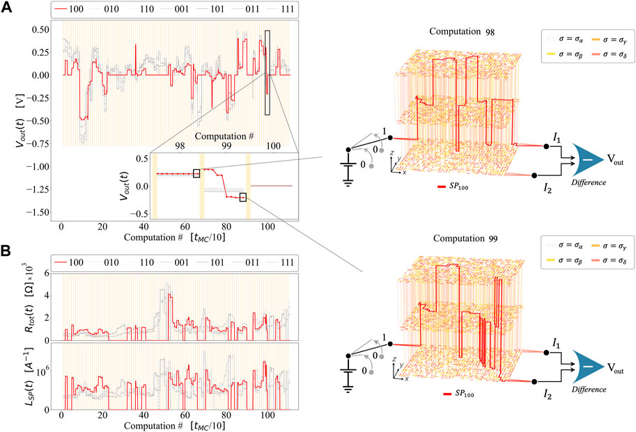
Figure 2. Simulation of the SRN model, in which each reprogramming is followed by a computation, repeating the process in series 110 times. During the simulation, the polarity and localization of the input channels in the reprogramming remain constant. Each computation lasts 10 MC steps. (A) Left panel: Evolution of
Shortest Paths, however, are not captured by their mere length: a visual inspection of their evolution is in fact quite instructive on the effects of specific reprogrammings and the topology of the induced network. An example is provided in the right panels of Figure 2A. Here we show how the reprogramming leaves the first section intact while inducing a notable change in the second part of the SPs for the (100) input combination configuration (red curve). It is precisely this latter variation that justifies the small difference between the outputs that decorate the overall trend. Even more interestingly, we observe a significant variability of SPs as a result of rearrangements. This indicates that extensive modifications of the inner structure are repeatedly occurring, in striking contrast to what is reported for a nanowire network (see, for example, [40]), where a single path was progressively strengthened. The repeated variation of outputs after reprogramming phases subtends a continuous change of the current SPs: such dynamics guarantees the reconfigurability of the device ad infinitum and preserves the variability of information processing resulting from such a ceaselessly mutating substrate.
Far from complete randomicity, however, such an evolution strongly depends on how the reprogramming is performed, thus on r. To prove this, we have analyzed, thanks to the Information Theory framework presented in [41, 42], the way in which reprogramming affects the information processing. The system is divided into 7 coarse-grained sub-regions (as shown in Figure 3A) to analyze the time-evolution of the electrical properties of each zone. Mutual Information (MI) associated with the electric current is used to describe the interactions among complementary areas of the system, while Integrated Information II) is exploited to evaluate the reciprocal integration among the building blocks of a sub-region [41, 42]. These measures are built on top of the entropy H, which is calculated from the discrete probability distribution of the average conductance in each sub-region (with 10 distinct states available to each coarse-grained zone; see Methods for details).
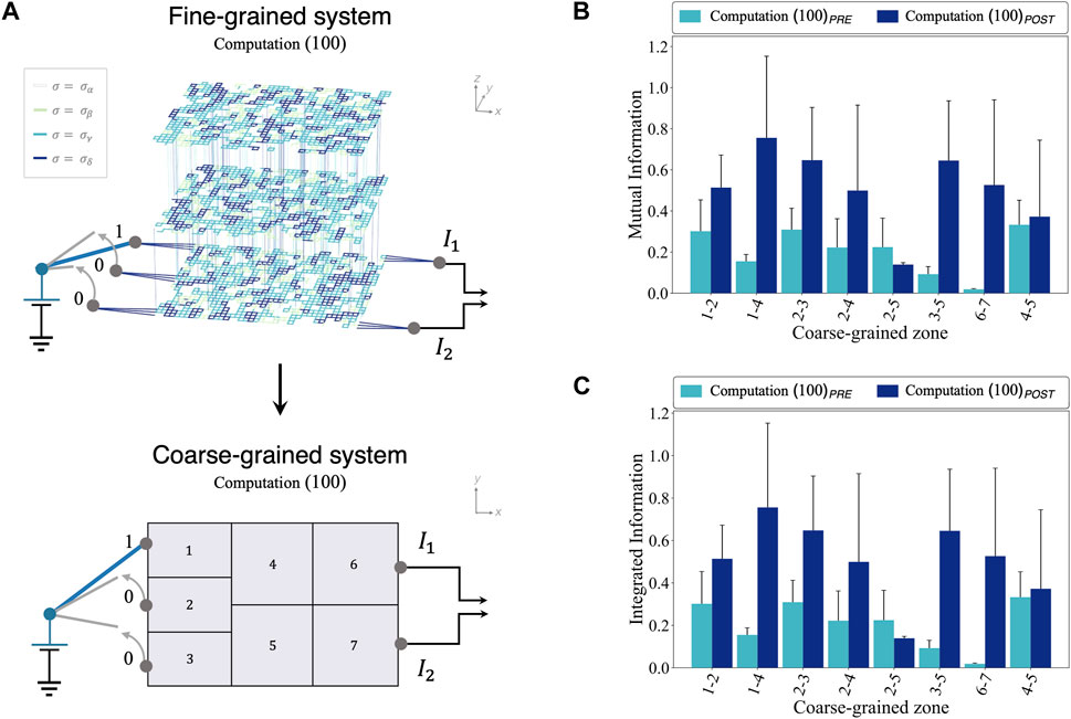
Figure 3. Left: network coarse-graining procedure (A). The coarse-grained system is obtained by dividing the network into seven parallelepipeds, each of which is mapped onto a two-dimensional sub-region. In both the schematic representations, the computation 100 is depicted. Right: The effect of a (1,0,0) reprogramming on Mutual Information MI (B) and Integrated Information II (C) between two or more coarse-grained sub-regions.
As shown in Figures 3A–C reprogramming with
On the other hand, since Mutual Information expresses the association between a part of the system and all the rest, we expect it to display a generalized growth after the reprogramming. This happens in most cases; the increase in 1–4 is marked, signaling an activation of such zones. Also 2–3, 2–5 and 3–5 exhibit a significant modification, probably because they are in closer contact with the 1–4 region where most of the variations in the electrical conduction happen. Supported by empirical evidence from this analysis, we can however state that different reprogramming input patterns result in partially altered levels of reciprocal correlations among sub-regions in the network, but more evidently in higher integration in the sub-regions closer to the open input channels. The spatial analysis of II and MI in the SRN can provide hints for the manipulation of hyperparameters of the reprogramming process, such as the amplitude, polarity, and localization of stimuli, in a way which is not applicable to the experimental electrical receptron.
3.2 Characterization of the receptron sampling efficiency
The indications provided by information theory can now be applied to the practical computation that we expect from receptron, finally analyzing its performances as a functional generator. To obtain a digitized output from an analog one, a thresholding procedure is exploited, where among a set of trial threshold values is retained the one which provides the greatest number of different generated functions [17]. The efficiency of the generation process will of course depend on the specific hardware implementation and on how the (stochastic) reprogramming is performed. We are first interested in determining which constructive characteristics have a higher impact on efficiency, while the effect of a specific reprogramming will be the object of the following section. A random exploration, where r is sampled from a uniform probability distribution stretching over the whole boundaries of the parameter space, allowed us to average out the contribution from the characteristics of the reprogramming.
The fact that a single receptron can generate any function [13], does not per se guarantee that it will do it quickly enough: such unconstrained opportunities would be useless if the device could not reach the desired target in a reasonable number of reprogrammings. In fact, the prohibitive scaling of the number of N-input Boolean functions (
We start by investigating which factors allow the maximization of the number of functions explored, while the next section will deal with targeting a specific area of the output functions space. The Boolean-function generation efficiency ε is a quantity already established for the experimental device [17], which for the case of 3 bits reduces to:
We have identified key mechanisms that influence this variability, acting on the evolution laws that are governing the dynamics of the computer-simulated receptron while using the physical one as a reference. Figure 4A compares distinct, i.e., regulated by a different dynamics, SRN-based implementations of a receptron, to be contrasted with the cyan experimental curve: the first type of network is composed of links that can explore 4 levels of conductance (blue curve), while in the second case only 2 states are possible (orange and red curves). In the latter cases, network’s links can access either a conductive level (respectively
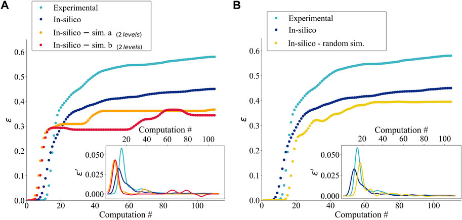
Figure 4. (A) Boolean function generation efficiencies (see Eq. 4) obtained for a an experimental receptron and different computer-simulated receptron, where we used a 4-levels SRN model (blue curve) and two 2-levels SRN model, each resulting by a random search process of a succession of 110 computations and reprogrammings. Inset: Derivatives of efficiency curves. (B) Efficiency and Derivatives computed for a physical receptron (turquoise curve), a computer-simulated receptron using an SRN model (blue curve), and a simulated receptron with randomly evolving topology (yellow curve) [29]. All curves have been smoothed using a 1D gaussian kernel.
The derivatives of the compared curves (inset) highlight that there is also a discrepancy between the saturation points and the different trends as a function of the computing step. While the qualitative behavior is shown to be insensitive to the details of the statistical evolution, some smaller quantitative differences arise in the shorter term for the derivative and in the longer term for the plateau value. These were used to settle the number of σ levels in simulations to 4 but also provides key insights into the functioning of such a system: its sampling efficiency strongly depends on the number of states accessible to each of the large number of conductances constituting the network.
Figure 4B compares the efficiency limiting values for both real and virtual receptrons: a physical receptron (cyan curve), a receptron simulated with the SRN model (blue curve), and a simulated receptron with randomly evolving topology - i.e., each link can be updated to one of the 4 conductance levels with uniform probability - (yellow curve). All the devices have similar efficiency trends, with an initial efficient exploration of the Boolean function space and a subsequent decrease of the variability and then of the curve slope. Even the simulated receptron with randomly evolving topology reaches a qualitatively comparable level of variability as the other two. Intuitively, the most significant differences between the various devices emerge after a few reprogramming steps: while it is relatively easy to generate new functions when only a tiny fraction of all the possibilities have already been visited, it becomes increasingly harder as reprogramming events start to accumulate. Thus, the key for a good receptron does not just lie in the number of degrees of freedom (which is enormous also in the case of the 2-level system) but rather in the availability of a wide set of local energy minima resulting in different outputs, in stark contrast with systems characterized by a Winner Takes it All dynamics [40], as we noted previously.
As discussed previously, however, the rate of generation of new functions is not a sufficient quantifier for the performance of this device: its ability to adapt to different reprogramming stimuli is critical if we are to limit its exploration to a much narrower target region of functional space. Being a global average, ε does not consider the second aspect, which is precisely where the physical behavior plays a crucial role, ensuring in principle the possibility to modify the statistical properties of the outputs: this is why we need to introduce controllability. We will now turn our attention to the quantification of this adaptability of the device, providing examples of parameters which determine different functional exploration.
3.3 Evaluation of the receptron controllability
Here we investigate the link between a specific reprogramming protocol and the resulting distribution of the outputs: as we anticipated,
A quantitative way to assess the receptron susceptibility to diverse reprogramming protocols consists in measuring the reprogramming/computing Mutual Information MI (R, F) [41, 42]: this will give indications on the effect of different stimuli sequences on the output function distributions. The Mutual Information between r and F,
We recall here that, while Eq. 2 well describes the possible ways to perform reprogramming in the experimental system, for the SRN model in its actual flavor the polarity is not a real degree of freedom: network configuration’s updates just depend on |
The results of this analysis are shown in Figure 5: the value of
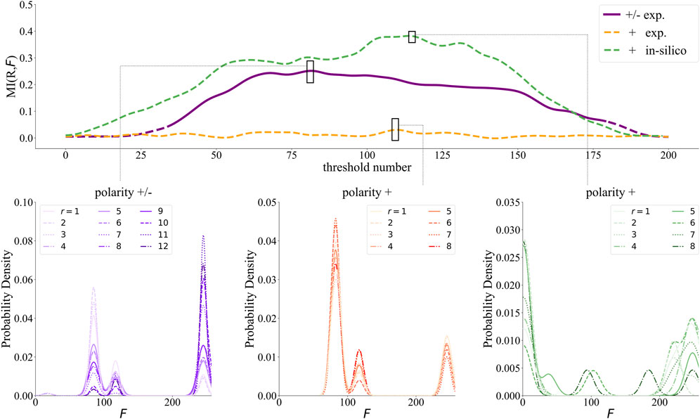
Figure 5. (Upper panel) Computation/reprogramming Mutual Information, MI (R, F) for different choices of r, indexed in an arbitrary way, on the same sample as a function of the chosen threshold (x-axis). The solid line indicates when MI is significant, while the dashed line indicates nonsignificance. For the experimental receptron the purple curve is obtained using positive and negative voltages during reprogramming steps, while the orange one (as the greenone for the SRN model) had the polarity fixed to just positive values. MI (R, F) curves have been smoothed with a Gaussian Kernel with
For a deeper understanding of what it does mean to have a non-significant MI (R, F) (i.e., vanishing), it is rather instructive to consider what happens for the extremal thresholds. Whenever the threshold lies very far from the analog weighted outputs’ mean, all thresholded outputs will be either 0 or 1, thus the output function will be forced to f = 0 ∨ f = 255 ∀ t (a Boolean function consisting of all zeros or ones, respectively): evidently, the specific series of reprogramming procedures, r, has no impact on the generated functions. Thus, even if the output function will be easily predicted, we have no control over the specific output function distribution: this first marks the distinction between our capability to predict
Intermediate thresholds allow the maximization of the MI curves. Notably, our experimental results reveal two different scenarios: the receptron consistently explores the same region within the space of Boolean functions for both fixed and variable polarity reprogramming protocols, resulting in non-significant and significant MI respectively. This is visually represented in Figure 5 - Bottom left and central panels, where we observe multimodal distributions with peaks precisely centered on the same output functions. We emphasize that the whole series of experimental measurements were conducted on the same device, with the primary difference being the random chronological order of the reprogrammings R) in each protocol. When we examine reprogramming protocols with a fixed positive polarity parameter (Figure 5 - Bottom central panel), our analysis shows that the output multi-mode distributions follows a consistent pattern, with the primary peaks reaching the same heights for each reprogramming mode. In this case, the output functions are not easily predicted (being the result of the system’s randomic dynamics), but still we cannot influence the outputs statistical likelihood by choosing specific reprogramming steps, which is rephrased in terms of a complete lack of controllability. More interestingly, when polarity truly makes a difference (Figure 5 - Bottom left panel), a different phenomenon emerges. In this case,
These examples highlight the difference between predictability and controllability: even if the system pertains to a degree of randomness (meaning it is not fully predictable), we can influence the statistics of the expected outcome via the specific features of reprogramming steps. The two quantities, however, evolve independently: as we have shown, we can have negligible controllability both in the case of high (for a trivial threshold setup) and low predictability (for positive-only polarity). Changing the polarity appears to be decisive for a nonzero controllability to emerge: this could be ascribed to a series of complex memory effects inside the cluster-assembled film, ranging from capacitive charge accumulation near the electrodes to bistable junction-switching, which are still under investigation. Conversely, we observe that the consequences of changing the reprogramming localization and the exact tension value have a smaller impact on the final outcome for different reasons. On the one hand, the numerical value of ∆V, beyond a given threshold, does not matter much (see also [18]); on the other hand, one expects a change in the reprogramming localization to be relevant but only limited to a sub-region of the system, as evidenced for the SRN by Figure 2. The results presented so far only allow us to limit the vast range of possible reprogramming protocols, but still, it is not feasible to quantitatively plan the reprogramming protocol to reach a specific target. To this extent, possible future improvements of the SRN, including an increased system responsivity after a polarity change, might help in further focusing on particular reprogramming protocols. All the analyses described so far leverage the Markovian hypothesis that a given reprogramming influences only the following one. However, we would expect higher levels of Mutual Information by considering as r the quantitative description of the reprogramming characteristics for n > 1 such steps: an analysis of this kind, however, requires further statistics, both in terms of the number of different reprogramming protocols and, fixing r, the number of reprogramming steps.
A future step will consist in the identification of a reasonable trade-off between increasing the accuracy of our predictions and the growing cost of such an approach. The analysis of temporal autocorrelation in our datasets suggests that the consequences of a reprogramming might, in principle, affect up to a few of the following readouts. The outputs’ trajectory in functional space is in fact the result (integral) of the contributions from several reprogramming steps: each one may be responsible for significant variations, but of course the starting point is itself dependent to some extent on the past history. In any case, the results presented so far, under assumption of Markovianity, already contribute to set some boundaries: we have underlined that only some hyperparameters are decisive to condition the system’s subsequent output. We argue the effect of such hyperparameters to have a larger relevance than the number of R sets explored.
4 Conclusion
We have successfully modeled the complex behavior of a physical receptron undergoing reprogramming and computing processes during the stochastic generation of Boolean functions. In particular, we have extended the characterization of the Boolean function generation process of a receptron to include not just efficiency measures but also a crucial controllability analysis. Aiming to quantitatively assess the effects of reprogramming on the network regions, we have employed Information Theory tools, highlighting the variable interacting strength with which different regions of the film react to external perturbations. We have discussed the requirements in terms of system size, thus number of junctions, for a sufficient level of complexity in the network: a large number of interconnected building blocks is needed together with the possibility for each of them to explore at least a few states (the discrete conductance levels). This complexity is reflected in the efficiency parameter, which captures the receptron intrinsic variability in generating Boolean output functions, together with the possibility to control its output, albeit in a statistical way.
Assessing the degree of controllability for a receptron is a key step in view of using it as a paradigm for innovative approaches to computing. Its inherent stochasticity, which lies at the heart of its flexibility and effectiveness, can in fact be limited by acting on the reprogramming process. We have identified reprogramming voltage polarity as a key parameter to steer the output functions distribution in the experimental receptron. The information obtained with this method provides the user with all the fundamental tools needed to calibrate the balance between predictability and controllability of the output values, with crucial influence on the device effectiveness as a Boolean function generator. Leveraging entropy-based measurements, we have developed a quantitative and robust criterion to determine which parameters allow the Mutual Information between the reprogramming protocol and the output to be significantly non-vanishing.
Even if qualitative, the agreement between the SRN model and the physical substrate is remarkable, the difference arising from the deep diversity of the two platforms, especially concerning fine details. Despite its considerable computational weight, the SRN is a coarse-grained physics-inspired abstract model, quite limited in size, much simpler than its experimental counterpart. Our simulations suggest that it is also more fragile upon repeated reprogramming steps: in the future, a systematic exploration of the grid of the SRN hyperparameters can undoubtedly help to increase the durability of the network.
Moreover, we plan to explore different strategies to implement a realistic dependence on the polarity of the applied tension in upcoming SRN developments, to better capture the experimentally assessed sensitivity to such hyperparameter. On the one hand, current SRN predictions concerning controllability provide generic indications about the relationship between a given reprogramming protocol and the resulting output vectors. On the other hand, while such results have a statistical robustness not comparable to the one typical of the experimental device, the simulation has a higher degree of reproducibility and often a lower cost than performing extensive experiments. Therefore, computational investigation can restrict the region of the phase space to be explored, allowing for more specific experimental campaigns. In addition, the simulations of the resistor network are useful to get insights about the experimental device functioning at a mesoscopic level: for instance, the visual inspection of current pathways, or the analysis of the reciprocal correlation among the different sub-regions. This kind of information is not retrievable from the mere analysis of the experimental receptron.
Data availability statement
The raw data supporting the conclusion of this article will be made available by the authors, without undue reservation.
Author contributions
ET: Conceptualization, Data curation, Formal Analysis, Funding acquisition, Investigation, Methodology, Software, Visualization, Writing–original draft. GM: Conceptualization, Data curation, Formal Analysis, Investigation, Methodology, Visualization, Writing–original draft. MM: Conceptualization, Methodology, Writing–review and editing. DG: Conceptualization, Funding acquisition, Methodology, Supervision, Writing–review and editing. PM: Conceptualization, Funding acquisition, Methodology, Software, Supervision, Writing–review and editing. FM: Conceptualization, Investigation, Methodology, Software, Supervision, Writing–original draft.
Funding
The author(s) declare that financial support was received for the research, authorship, and/or publication of this article. The study was also supported by the CINECA agreement with Università degli Studi di Milano 2019–2020, CINECA grants IscraC RENNA 2019 and IscraC iRENNA 2021 and INDACO-UNITECH 2020–2022. These organizations provided high-performance computing resources and technical support that were crucial for the successful completion of the research.
Acknowledgments
The authors thank Michele Allegra for his contributions during the development of this work, providing valuable insights and suggestions that helped shape the final product.
Conflict of interest
The authors declare that the research was conducted in the absence of any commercial or financial relationships that could be construed as a potential conflict of interest.
Publisher’s note
All claims expressed in this article are solely those of the authors and do not necessarily represent those of their affiliated organizations, or those of the publisher, the editors and the reviewers. Any product that may be evaluated in this article, or claim that may be made by its manufacturer, is not guaranteed or endorsed by the publisher.
Supplementary material
The Supplementary Material for this article can be found online at: https://www.frontiersin.org/articles/10.3389/fphy.2024.1400919/full#supplementary-material
References
1. Teuscher Christof. Unconventional computing catechism. Front Robotics AI (2014) 1:10. doi:10.3389/frobt.2014.00010
2. Dale M, Miller JF, Stepney S Advances in unconventional computing: volume 1: theory. Berlin, Heidelberg: Springer (2017).
3. Schrauwen B, Verstraeten D, Van Campenhout J. An overview of reservoir computing: theory, applications and implementations. In: ESANN 2007 Proceedings - 15th European Symposium on Artificial Neural Networks; April 25-27, 2007; Bruges, Belgium (2007).
4. Verstraeten D, Schrauwen B, D’Haene M, Stroobandt D. An experimental unification of reservoir computing methods. Neural Networks (2007) 20(3):391–403. doi:10.1016/j.neunet.2007.04.003
5. Tanaka G, Yamane T, Héroux JB, Nakane R, Kanazawa N, Takeda S, et al. Recent advances in physical reservoir computing: a review. Neural Networks (2019) 115:100–23. doi:10.1016/j.neunet.2019.03.005
6. Dale M, Miller JF, Stepney S, Trefzer MA. A substrate-independent framework to characterize reservoir computers. Proc R Soc A: Math Phys Eng Sci (2019) 475(2226):20180723. doi:10.1098/rspa.2018.0723
7. Banda P, Teuscher C, Lakin MR. Online learning in a chemical perceptron. Artif Life (2013) 19(2):195–219. doi:10.1162/ARTL_a_00105
8. Miller JF, Harding SL, Tufte G. Evolution-in-materio: evolving computation in materials. Evol Intelligence (2014) 7(1):49–67. doi:10.1007/s12065-014-0106-6
9. Larger L, Baylón-Fuentes A, Martinenghi R, Udaltsov VS, Chembo YK, Jacquot M. High-speed photonic reservoir computing using a time-delay-based architecture: million words per second classification. Phys Rev X (2017) 7(1):011015. doi:10.1103/PhysRevX.7.011015
10. Miller JF, Downing K. Evolution in materio: looking beyond the silicon box. In: Proceedings - NASA/DoD Conference on Evolvable Hardware, EH (2002).
11. Indiveri G. Introducing ‘neuromorphic computing and engineering. Neuromorphic Comput Eng (2021) 1(1):010401. doi:10.1088/2634-4386/ac0a5b
12. Li Q, Diaz-Alvarez A, Iguchi R, Hochstetter J, Loeffler A, Zhu R, et al. Dynamic electrical pathway tuning in neuromorphic nanowire networks. Adv Funct Mater (2020) 30(43). doi:10.1002/adfm.202003679
13. Paroli B, Martini G, Potenza MAC, Siano M, Mirigliano M, Milani P. Solving classification tasks by a receptron based on nonlinear optical speckle fields. Neural Networks (2023) 166:634–44. doi:10.1016/j.neunet.2023.08.001
14. Minsky M, Papert S Perceptron: an introduction to computational geometry, 19. Cambridge: The MIT Press (1969). expanded edition.
15. Lecun Y, Bengio Y, Hinton G. Deep learning. Nature (2015) 521(7553):436–44. doi:10.1038/nature14539
16. Martini G, Mirigliano M, Paroli B, Milani P. The Receptron: a device for the implementation of information processing systems based on complex nanostructured systems. Jpn J Appl Phys (2022) 61:SM0801. doi:10.35848/1347-4065/ac665c
17. Mirigliano M, Paroli B, Martini G, Fedrizzi M, Falqui A, Casu A, et al. A binary classifier based on a reconfigurable dense network of metallic nanojunctions. Neuromorphic Comput Eng (2021) 1(2):024007. doi:10.1088/2634-4386/ac29c9
18. Mambretti F, Mirigliano M, Tentori E, Pedrani N, Martini G, Milani P, et al. Dynamical stochastic simulation of complex electrical behavior in neuromorphic networks of metallic nanojunctions. Sci Rep (2022) 12(1):12234. doi:10.1038/s41598-022-15996-9
19. Minnai C, Bellacicca A, Brown SA, Milani P. Facile fabrication of complex networks of memristive devices. Sci Rep (2017) 7(1):7955. doi:10.1038/s41598-017-08244-y
20. Mirigliano M, Borghi F, Podestà A, Antidormi A, Colombo L, Milani P. Non-ohmic behavior and resistive switching of Au cluster-assembled films beyond the percolation threshold. Nanoscale Adv (2019) 1(8):3119–30. doi:10.1039/c9na00256a
21. Mirigliano M, Decastri D, Pullia A, Dellasega D, Casu A, Falqui A, et al. Complex electrical spiking activity in resistive switching nanostructured Au two-terminal devices. Nanotechnology (2020) 31(23):234001. doi:10.1088/1361-6528/ab76ec
22. Tarantino W, Colombo L. Modeling resistive switching in nanogranular metal films. Phys Rev Res (2020) 2(4):043389. doi:10.1103/PhysRevResearch.2.043389
23. López-Suárez M, Melis C, Colombo L, Tarantino W. Modeling charge transport in gold nanogranular films. Phys Rev Mater (2021) 5(12):126001. doi:10.1103/PhysRevMaterials.5.126001
24. Nadalini G, Borghi F, Košutová T, Falqui A, Ludwig N, Milani P. Engineering the structural and electrical interplay of nanostructured Au resistive switching networks by controlling the forming process. Sci Rep (2023) 13:19713. doi:10.1038/s41598-023-46990-4
25. Casu A, Chiodoni A, Ivanov YP, Divitini G, Milani P, Falqui A. In situ TEM investigation of thermally induced modifications of cluster-assembled gold films undergoing resistive switching: implications for nanostructured neuromorphic devices. ACS Appl Nano Mater (2024) 7(7):7203–12. doi:10.1021/acsanm.3c06261
26. Strukov DB, Stanley Williams R. Exponential ionic drift: fast switching and low volatility of thin-film memristors. Appl Phys A (2009) 94(3):515–9. doi:10.1007/s00339-008-4975-3
27. Durkan C, Welland ME, Welland ME. Analysis of failure mechanisms in electrically stressed Au nanowires. J Appl Phys (1999) 86(3):1280–6. doi:10.1063/1.370882
28. Mirigliano M, Milani P. Electrical conduction in nanogranular cluster-assembled metallic films. Adv Phys (2021) 6. doi:10.1080/23746149.2021.1908847
29. Kagan M. On equivalent resistance of electrical circuits. Am J Phys (2015) 83(1):53–63. doi:10.1119/1.4900918
30. Rubido N, Grebogi C, Baptista MS. General analytical solutions for DC/AC circuit-network analysis. Eur Phys J ST, Spec Top (2017) 9. doi:10.1140/epjst/e2017-70074-2
31. Montano M, Milano G, Ricciardi C. Grid-graph modeling of emergent neuromorphic dynamics and heterosynaptic plasticity in memristive nanonetworks. Neurom. Comput. Eng (2023) 2:014007. doi:10.1088/2634-4386/ac4d86
32. de Arcangelis L, Redner S, Herrmann HJ. A random fuse model for breaking processes. J de Physique Lettres (1985) 46(13):585–90. doi:10.1051/jphyslet:019850046013058500
33. Costagliola G, Boisa F, Pugno NM. Random fuse model in the presence of self-healing. New J Phys (2020) 22:033005. doi:10.1088/1367-2630/ab713f
34. Zhu R, Hochstetter J, Loeffler A, Diaz-Alvarez A, Nakayama T, Lizier JT, et al. Information dynamics in neuromorphic nanowire networks. Sci Rep (2021) 11:13047. doi:10.1038/s41598-021-92170-7
36. Cover TM, Thomas JA. Entropy, relative entropy, and mutual information. In: Elements of information theory (2005). doi:10.1002/047174882x.ch2
37. Roulston MS. Estimating the errors on measured entropy and Mutual Information. Physica D (1999) 125(3–4):285–94. doi:10.1016/S0167-2789(98)00269-3
38. Dijkstra EW. A note on two problems in connexion with graphs. Numer Math (Heidelb) (1959) 1(1):269–71. doi:10.1007/BF01386390
39. NetworkX. NetworkX. Available from: https://github.com/networkx/networkx (Accessed October 26, 2023).
40. Manning HG, Niosi F, da Rocha CG, Bellew AT, O’Callaghan C, Biswas S, et al. Emergence of winner-takes-all connectivity paths in random nanowire networks. Nat Commun (2018) 9(1):3219. doi:10.1038/s41467-018-05517-6
41. Sporns O, Tononi G, Kötter R. The human connectome: a structural description of the human brain. PLoS Comput Biol (2005) 1(4):e42. doi:10.1371/journal.pcbi.0010042
Keywords: receptron, stochastic resistor network, unconventional computing, boolean functions, nanostructured films
Citation: Martini G, Tentori E, Mirigliano M, Galli DE, Milani P and Mambretti F (2024) Efficiency and controllability of stochastic boolean function generation by a random network of non-linear nanoparticle junctions. Front. Phys. 12:1400919. doi: 10.3389/fphy.2024.1400919
Received: 20 March 2024; Accepted: 25 April 2024;
Published: 30 May 2024.
Edited by:
Matteo Cirillo, University of Rome Tor Vergata, ItalyReviewed by:
Paolo Moretti, University of Erlangen Nuremberg, GermanyThomas Cusick, University at Buffalo, United States
Copyright © 2024 Martini, Tentori, Mirigliano, Galli, Milani and Mambretti. This is an open-access article distributed under the terms of the Creative Commons Attribution License (CC BY). The use, distribution or reproduction in other forums is permitted, provided the original author(s) and the copyright owner(s) are credited and that the original publication in this journal is cited, in accordance with accepted academic practice. No use, distribution or reproduction is permitted which does not comply with these terms.
*Correspondence: P. Milani, cGFvbG8ubWlsYW5pQHVuaW1pLml0; D. E. Galli, ZGF2aWRlLmdhbGxpQHVuaW1pLml0
†These authors have contributed equally to this work
‡ORCID: P. Milani, orcid.org/0000-0001-9325-4963; D. E. Galli, orcid.org/0000-0002-1312-1181; M.Mirigliano, orcid.org/0000-0002-6435-8269