Poloidally asymmetric potential formation on plasma boundary in axisymmetric magnetic field

To study the symmetry of electrical potential, we model plasma transport in the edge region of a toroidal device with two spatial dimensions (2D) and three coordinates for velocities (3V) using a Particle-In-Cell (PIC) code. A two-dimensional magnetic field is applied, including poloidal and toroidal components, which are periodic in the poloidal direction. We discover relationships between the magnetic gradient drift and potential formation using PIC simulation, which has not been captured in other numerical models. We find that the inverse aspect ratio influences the asymmetry of the potential in an axisymmetric magnetic configuration.

1 Introduction

In magnetically confined plasmas, particles move along a magnetic field line, making a circular gyro motion with the Larmor radius. The magnetic field becomes one of the key factors influencing the particles’ orbit and transport. Generally, the magnetic field lines in the edge plasma region of fusion devices are changed from closed to open. Therefore, physical behaviors in the edge plasma are complicated. Moving along the open field lines, particles are lost at the material surface, which is connected directly with these field lines. Having higher thermal velocity and being lighter than ions, losses of electrons in the open field line are not the same as those of the ions. Based on this imbalance, the electric field is self-consistently generated, breaking the charge neutrality in the edge region. In a large aspect ratio limit system where strong toroidicity is included, the particles drift off the magnetic flux surface due to the presence of grad-B and curvature drifts [1]. The neoclassical effect, which includes the effects of the toroidal geometry, changes the plasma transport coefficients. When anomalous transport and turbulence effects are not considered, the grad-B drift induced by the toroidicity becomes a critical element affecting perpendicular particle transport. The velocity of the grad-B drift has the opposite signs for the electrons and ions. Subsequently, their movements are contradictory. As a result, the grad-B drift can be considered one of the candidates to break down the symmetric behavior of the particle transport in the axisymmetric magnetic field system. Several experimental and numerical studies have recently shown the relationship between the potential profile and magnetic field [2–7]. In these works, the fluid description was widely used to compute the electrical potential. However, none studied the asymmetry of the potential profile. It was mainly because the fluid theory could not precisely include drift effects. Finally, only symmetric potential profiles were obtained in these works.

$\mathbf{E}\times \mathbf{B}$ and $\mathbf{B}\times \mathbf{\nabla }\text{B}$ drifts are included in a fully kinetic description. This work uses a kinetic theory instead of the drifts theory to study the asymmetric potential formation in the axisymmetric system. The Particle-In-Cell (PIC) simulation, which uses the fully kinetic description, can deal with drift explicitly and compute particle gyro-motion exactly, compared with other fluid models [8]. The $\mathbf{E}\times \mathbf{B}$ and $\mathbf{B}\times \mathbf{\nabla }\text{B}$ drifts are treated in the equations of motion. Particles leave the plasma core by drifting outward from the Last Closed Flux Surface (LCFS). The physics of the edge plasma can be determined by ion orbit loss which affects the distribution of the particles and hence changes the physics properties [9]. Understanding the mechanisms of the ion orbit loss or particle loss helps explain the physics phenomenon in the edge plasma.

This paper discusses how the grad-B drift affects the symmetry of the potential profiles in the edge region. A flow of plasma in the edge region containing ions and electrons is modeled in two spatial and three velocity coordinates (2D3V) by using a PIC simulation. Different values of the inverse aspect ratio are applied to adjust the strength of the drift effects on particle motion. The scope of this study is to find a suitable explanation for the asymmetric potential formation in the presence of the axisymmetric magnetic field configuration.

The paper is organized as follows. The model and initial conditions for simulation setup are described in Section 2. A transformation of the cross-section of toroidal limiters to slab geometry is presented. This slab model is easier to use than torus geometry for numerical analysis of particle transport near the LCFS. We studied the influences of the inverse aspect ratio on the potential profiles. Our goal is to understand the formation of asymmetric potential in the axisymmetric magnetic field. Therefore, the boundary conditions at the core region and limiter wall have not been precisely included in this work compared with any realistic devices. Section 3 shows the effect of the grad-B drift on particle motion. The change in particle transport influences the formation of the potential. The dependencies of the asymmetric potential formation on the inverse aspect ratio are analyzed. A summary and conclusion of this work are discussed in the last section.

2 Simulation model

We aim to concentrate on the self-consistent formation of the electric field and electrical potential under the effects of toroidicity rather than the time evolution of the magnetic field. Therefore, in this work, the electrostatic model is preferable to use instead of the electromagnetic one. The electric field E is self-consistently computed, and the magnetic field B is constant in time. The main Equations 1–4 use in the electrostatic PIC simulation are given as [8, 10]:

$\frac{d\mathbf{x}}{dt}=\mathbf{v},(1)$

$m_s\frac{d\mathbf{v}}{dt}=q_s^{\text{c}}\left(\mathbf{E}+\mathbf{v}\times \mathbf{B}\right),(2)$

$\mathbf{E}=-\mathbf{\nabla }\varphi ,(3)$

${\mathbf{\nabla }}^2\varphi =-\frac{\rho }{{ϵ}_0}=-\frac{1}{{ϵ}_0}{\displaystyle \sum _s}{q}_s^{\text{c}}{n}_s,(4)$

where $\mathbf{x}$, $\mathbf{v}$, $q_s^{\text{c}}$, $n_s$ and $m_s$ are the position, velocity, charge, density, and mass of the species $s$, respectively. $\mathbf{E}$, $\mathbf{B}$, $\varphi$, and $\rho$ represent the electric field, the magnetic field, the electric potential, and the charge density, respectively. Particle positions and field quantities are considered in two-dimensional spaces ($x$, $y$) with three components of velocity $(v_x,v_y,v_z)$ (2D3V). These equations are solved by using the finite different method. The leap-frog scheme and Boris rotation are used in solving equations of motion [8]. The Poisson’s equation can be solved by applying the successive-over relaxation method. The field can be obtained in each spacial grid. We applied the numerical methods proposed by Birdsall for solving these equations, integrating the field and accumulating the charge [8, 10]. After assigning some initial values for particles’ velocities and positions, at each time-step, the simulation accumulates the charge and compute the field on each grid by solving the Poisson’s equation. Then, the electric and magnetic fields are used to calculate the force acting on each particle. Particles’ velocities and positions are updated by using this force. Boundary conditions is also checked in this step. These step are repeated until the simulation reaches the equilibrium stage where all of the fields remain stable.

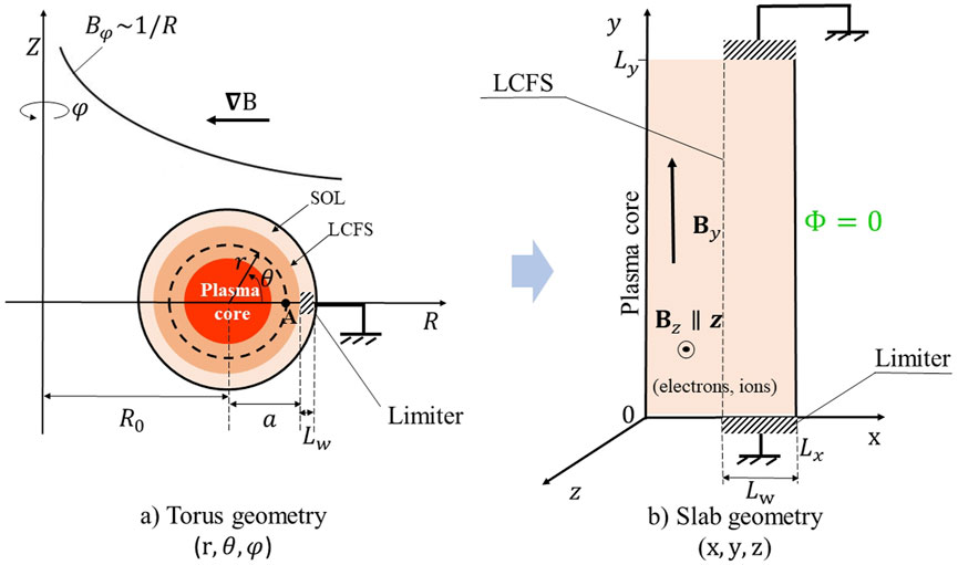
A single, flat-sided toroidal ring limiter plasma is considered. We study a small region near the LCFS, including the inside and outside regions of the LCFS. The magnetic field lines are closed inside the LCFS and opened in the Scrape-Off Layer (SOL) region. In the SOL region, they connect to the limiters. To be simpler in numerical analysis, the SOL has been straightened out; the torus geometry is transferred to a two-dimensional slab geometry, as shown in Figure 1 [11, 12]. Figure 1A) shows the poloidal cross-section of the torus geometry, while Figure 1B) illustrates the transferred slab geometry, which has been used in this work. The shape and materials of the limiter are ignored. The thickness of the studied domain is twice that of the limiter length. Point A in the torus geometry corresponds to the origin of the slab geometry. The size of the simulation domain is set up as $L_x=0.06$ m, including $L_{\text{w}}=0.03$ m, which is the length of the limiter, and $L_y=1.0$ m. We suppose the limiter is connected with the ground, and the electric potential at $x=L_x$ is zero. At $x=0$, the electric potential is assumed to satisfy floating potential conditions. For clarification, we define the left, right, bottom, and top boundaries as $x=0$, $x=L_x$, $y=0$, and $y=L_y$, respectively. Inside the LCFS where $x<x_{\text{w}}$ (where $x_{\text{w}}=L_x-L_{\text{w}}$), a periodic boundary condition is used at the top and bottom boundaries. A particle that quits the simulation domain from these periodic boundaries at the time $t$, has a new position $y_{\mathit{new}}^t=y_{\mathit{old}}^t-L_y$ for $y^t>L_y$ for $y_{\mathit{new}}^t=y_{\mathit{old}}^t+L_y$ for $y^t<0$, while keeping the $x$ position and its velocities the same. A real mass ratio of ions and electrons in a Hydrogen plasma, $m_i/m_e=1836$, is employed in this simulation. Therefore, the physics of electrons and ions are captured in our simulation more realistically. Several types of collisions may occur in the plasma edge, including those between charged particles, charged particles with neutrals, and charged particles with impurities. In this study, only electrons and ions are considered. No neutral particle or impurity has been included. Only the collision between charged particles is added, which is approximated by the Monte Carlo method. The Coulomb collision between ion-ion, electron-electron, and electron-ion is covered. We apply Nanbu’s theory to treat the Coulomb collision as a successive binary collision [13, 14]. The sufficiently short time step and sufficiently large number of the simulated particles are carefully chosen in the simulation to get the high accuracy when using Nanbu’s model. Values of the time step and number of the simulated particles per cell are given in the last paragraph of this section.

Figure 1

Figure 1. Simulation domain. Figure (A) shows the torus geometry of the toroidal limiter, while Fig. (B) displays the transferred two-dimensional slab geometry used in the simulation. The simulation domain is the region from the dashed line to the solid line in the torus geometry. The origin in the slab coordinates denotes a location at $R=(R_0+a+L_{\text{w}})-L_x$ in the torus coordinates (point A). The limiters are connected to the ground.

This work studies the asymmetry of potential formation in the axisymmetric magnetic field system. The simulation domain and magnetic profiles are set up to be symmetric via the mid-line $y=L_y/2$. The radial, poloidal and toroidal magnetic field ($B_r$, $B_{\theta }$, $B_{\phi }$) in a torus correspond to ($B_x$, $B_y$, $B_z$) in the two-dimensional slab geometry, respectively. Generally, in a torus, the field includes toroidal effects. A toroidal magnetic field is proportional to $1/R$. The toroidal magnetic field is strongest at the center of the torus and weakest on its outside. According to Figure 1A), the toroidal magnetic field is weaker from the left to the right-hand side and is equal for all locations with the same $R$. Subsequently, in the slab model, the magnetic field $B_z$ should be higher in the middle of the simulation box in the $y$ direction and smaller near the limiters. The poloidal magnetic field in the torus depends on the distance to the center of the plasma core. Consequently, the poloidal and toroidal magnetic field in the torus geometry can be approximately transferred to the slab system as:

$\begin{array}{c}\hfill B_{\theta }=\frac{r{B}_{\phi }}{R_0{q}_s}\to B_y=\frac{B_{0y}a}{2+2{\left(\frac{x+a-x_{\text{w}}}{a}\right)}^2},\\ \hfill B_{\phi }=B_{0z}\left(1-ϵ\cos \theta \right)\to B_z=B_{0z}\left[1-\frac{x+a-x_{\text{w}}}{R_0}\cos \left(\frac{2\pi y}{L_y}\right)\right],\end{array}(5)$

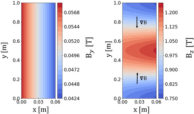
where $a$ and $R_0$ are the minor and major radii of the torus, $ϵ=a/R_0$ is the inverse aspect ratio, $B_{0y}$ and $B_{0z}$ are the applied magnetic field (choosing $B_{0y}=B_{0z}=1.0$ T). The safety factor $q_s$ is added in the poloidal magnetic field formula to include the toroidal current. In this simulation, the safety factor is set to be equal to 2. The transferred formulas of the magnetic field $B_y$ and $B_z$ are chosen to be the most related to the torus system. The radial or magnetic field in the $x$ direction is not included (i.e., $B_x=0$ T). We aim to see how particles can transport in the radial direction, even though no magnetic field occurs in this direction. Figure 2 illustrates the magnetic field profile. Since the poloidal magnetic field related to the safety factor is added to the simulation, the effect of the toroidal current on the poloidal field is included. The toroidal magnetic field $B_z$ is symmetric in the $y$ direction via the midline $y=L_y/2$. This magnetic field profile includes the toroidal gradient and curvature drift, similar to the torus geometry.

Figure 2

Figure 2. The poloidal (i.e., $B_y$) and toroidal magnetic field (i.e., $B_z$) in the simulation domain. These magnetic field profiles correspond with the poloidal and toroidal magnetic field in the torus geometry, in which the curvature drift and toroidal gradient are included. $B_y$ is dependent only on the $x$ position, while $B_z$ is symmetric in the $y$ direction from the mid-line $y=L_y/2$. The gradient of the toroidal magnetic field has the opposite direction via the mid-line.

Linked to the torus geometry, the left boundary is the closest to the plasma core compared to other regions. The particle densities and temperatures around this boundary should be higher than in other locations. The initial profiles of particle density $n_s$, and temperature $\text{k}{T}_s$ of species $s$ are proposed as:

$n_s\left(x\right)=n_{s,0}\exp \left(-\frac{x-x_{\text{w}}}{{\lambda }_n}\right),\text{k}{T}_s\left(x\right)=\text{k}{T}_{s,0}\exp \left(-\frac{x-x_{\text{w}}}{{\lambda }_{\text{k}T}}\right),(6)$

where ${\lambda }_n$ and ${\lambda }_{\text{k}T}$ are the scale lengths for the density and temperature profiles (choosing ${\lambda }_n=0.02$ m, ${\lambda }_{\text{k}T}=0.03$ m), and $n_0$ and $\text{k}{T}_0$ are the particle density and temperature at the LCFS, respectively. These equations depend only on the $x$ direction and have an exponential profile. This exponential profile is chosen to map the particle densities and temperatures in the simulation as similar to those in the H-mode [15–19]. Even though a simple simulation model has been established for the present numerical study, we try to include as much similarity in the particle profiles and drift effects as those covered in the theory and experiments as possible. Hence, although none of the exact values of any real devices is used in the simulation, the physics phenomena of particles obtained from this simple simulation system can still be used to analyze the basic physics phenomena near the LCFS. Taken from the initial temperature of particles, their initial velocities satisfying a fully Maxwellian distribution can be computed, based on the Box-Muller algorithm. We assign an equal density at the LCFS for electrons and ions in all the simulations in this study, choosing $n_0=4\times 10^{17}$ ${\text{m}}^{-3}$. Electrons and ions are assumed to have the same temperature at the LCFS, $\text{k}{T}_0=200$ $\text{eV}$. Given these initial values, at the region $x=0$ and $y=L_y/2$, the system size can be equivalent to $L_x\approx 464{\lambda }_D\approx 12r_{L,i}$ where ${\lambda }_D$ and $r_{L,i}$ are the Debye length and ion Larmor radius, respectively. After having the initial particles’ positions and velocities, the particles’ positions and velocities will be updated each time-step in PIC simulation. Once the particles are moving along the simulation box, they may escape from the simulation box at four boundaries. The total number of particles reduces at each time step. To consider the charge neutrality and conservation of mass, the total number of particles is assumed to be constant in time. To do that, besides the mentioned periodic condition, we add other types of boundary conditions into the simulation. First, those particles having a negative position in the $x$ direction at the time $t$ are reflected back immediately into the simulation box following regular reflection. Only the position and velocity in the $x$ direction are inversely changed. Another state is the injection condition, which is applied to particles leaving the simulation domain at the end boundary and the limiters. Particles are fully absorbed at the limiters and the end boundary where $x=L_x$. Once a particle is lost at these boundaries, a new one is injected into the simulation in the inside LCFS region. A random position is chosen to avoid instabilities [20]. Its thermal velocity satisfies the initial temperature function, as in Equation 6.

Parallelization programming is necessary for operating this simulation to reduce the running time. Our program is parallelized using Message Passing Interface (MPI). It runs in the Plasma Simulator of the National Institute for Fusion Science, Japan: the NEC SX-Aurora TSUBASA supercomputer with 64 cores. The number of cells, time step, and other parameters are chosen to satisfy the stability condition of the PIC simulation. To reduce noise when capturing physics behaviors at a certain time, time averaging of all quantities in 100 time steps is applied in the post-process. The total numbers of cells in the $x$ and $y$ directions are set to be $N_{cx}=480$ cells, $N_{cy}=8000$ cells, respectively. The time step $\mathrm{\Delta }t$ is chosen as $\mathrm{\Delta }t=0.2{\omega }_{p0}^{-1}$ where ${\omega }_{p0}$ is the plasma frequency computed at the boundary $x=0$. Each cell carries 256 simulated particles at this boundary at the initial stage. Following the properties of the exponential function, plasma density and temperature are highly concentrated inside the LCFS, and those values become lower on the outside. The diffusion process of high-energetic particles may occur. Because of no magnetic field in the $x$ direction, particles will likely move along the magnetic field lines in the $y$ direction, reaching the limiter wall. Thanks to the presence of the toroidal drifts and collisions between charged particles, the particle transport in the $x$ direction (i.e., the radial direction) is induced. This is mainly because the toroidal drifts can move the transport perpendicularly, and the collisions generate movement in a random direction. The particle displacement under the Coulomb collision is in the order of a Larmor radius $r_L=m{v}_{\perp }/|q|B$ [1, 21, 22]. Changing the particle Larmor radius may affect the transport of particles in the radial direction. Because collision creates random walk, high collisionality strongly affects transport in the radial direction, causing a drastic diffusion of particles. Collisions become the dominant effects causing the particle transport in the system. Collisional effects may be statistically inaccurate for higher collision frequencies in the present Monte-Carlo model. We assume low collisionality to consider the collisional effects qualitatively, using a reasonable time-step interval. The collision is called every 100 time step in which the total energy of particles after a collision occurs is still conserved. Different charges, masses, and velocities make the movement of electrons and ions under the drift effects and collisions different. The electric field is self-consistently generated, corresponding to this unequal movement. The potential profiles, thereafter, should reflect the difference between the transport of electrons and ions. The next section shows the particle behaviors captured after running at a certain time, $N_t=\mathrm{30,000}$ time steps. The particles continue diffusing with time after this period, but they keep the same tendency of movement. Therefore, results at this particular time are acceptable for analyzing the effect of the drifts and Larmor radius on the particle motion.

3 Simulation results

Separated by the mid-line $y=L_y/2$, the lower region is defined as that from 0 to $L_y/2$, while the upper one is from $L_y/2$ to $L_y$. The magnetic field $B_z$ depends on the location in the $y$ direction. It is symmetric, localized, and has a peak value at the middle region in the $y$ direction. As a result, the gradient of the toroidal magnetic field has the opposite direction, as given in Figure 2. Subsequently, the effect of the grad-B drift on particle transport is inverse between the upper and lower regions. The drift is perpendicular to ${\mathbf{B}}_{\mathbf{z}}$ and $\nabla B_z$, which is the $x$ direction. There is a possibility that a particle moves in the radial direction if the grad-B drift is included. The grad-B drift velocity ${\mathbf{v}}_{\nabla B}$ can be computed as [23]:

${\mathbf{v}}_{\nabla B}=\pm \frac{1}{2}{v}_{\perp }{r}_L\frac{\mathbf{B}\times \nabla B}{B^2},(7)$

where $\pm$ stands for the sign of charge. In the case of fixed particle velocities, the grad-B drift depends on the strength of the gradient in $|B|$. As given in Equation 5, the toroidal magnetic field corresponds to the factor $a/R_0$, in other words, the inverse aspect ratio. When the system has a large inverse aspect ratio, the toroidal magnetic field is strongly different at every point along the simulation domain; the gradient of the magnetic field is strong. The toroidal magnetic field will be approximately constant if the inverse aspect ratio is minimal. In this case, the grad-B drift is almost zero and can be ignored. To study the effect of the grad-B drift, we adjust its strength on particles by changing the inverse aspect ratio or the major radius $R_0$. The value of the minor radius is fixed for all simulations (choosing $a=0.2$ m). We test for both cases where a very strong and approximately zero grad-B drift occurs in the system.

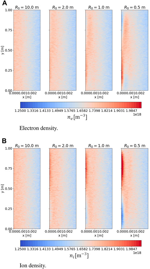
First, let us consider the movement of ions near the left boundary. In a case without considering the effect of $B_y$, the ions spiral clockwise when the magnetic field $B_z$ is in the outward direction. As discussed in Section 2, a reflection condition is applied for particles leaving the simulation box from the left boundary. Once the ions hit the left boundary, they are reflected. These re-entering ions will move downward when composing the gyro motion. From the mid-line $y=L_y/2$ to the bottom boundary, the magnetic field $B_z$ decreases. Hence, the instantaneous Larmor radius for the ions will become larger when they move downward. There are more chances for large Larmor radius ions to leave the simulation domain from the bottom boundary. Once quitting the bottom boundary, because of the periodic condition, these large Larmor radius ions will enter the upper region in the simulation box. Here, ions at the left boundary also move downward. However, they move from a low magnetic field to a strong one, where the Larmor radius becomes smaller. It is hard for the small Larmor radius ions to jump from the upper to the lower region. The ions near the left boundary are mostly located in the upper region. Consequently, the ion density there is higher than that in the lower region. A similar mechanism is obtained for the electron transaction. Electrons have the opposite sign of charge and spiral counter-clockwise in the presence of outward $B_z$. The transport of the electrons will be inverse as compared to that of the ions. Electrons tend to move upward after reflecting at the left boundary. Large Larmor radius electrons can move from the upper to the lower region via the top boundary by the periodic condition. In comparison, those in the lower region do not easily enter the upper region because of their small Larmor radius. As a result, the electron density in the upper region at the left boundary is lower than in the lower one. As seen from Equation 7, the grad-B drift is in the opposite directions for the electrons and ions. Therefore, electron and ion transports are opposite under the grad-B drift effect. The ions tend to move to the left boundary in the lower region since the $\nabla \text{B}$ has a positive direction in this region. In contrast, the electrons are more likely to move to the LCFS. In the upper region where negative $\nabla B$ is located, the movement of the electrons and ions is the inverse of the lower region. Therefore, the grad-B drift forces more ion loss at the left boundary in the lower region and causes more electron loss in the upper region at this boundary. Increasing the loss of particles at the left boundary raises the number of reflected particles. More ions (electrons) jump from the lower (upper) region to the upper (lower) one. Subsequently, the polarity of particle densities between the upper and lower region becomes more obvious if the grad-B drift is stronger. The effects of $\mathbf{B}\times \mathbf{\nabla }\text{B}$ drift on particle transport are obtained in PIC simulation, as illustrated in Figure 3. This figure shows a shortcut in the simulation domain of several millimeters from the left boundary where the difference is clearest. When a large major radius is used, the toroidal magnetic field is almost constant, resulting in extremely small grad-B drift. Only a few particles are lost at the left boundary. The difference in electron and ion densities between the upper and lower regions is invisible, as seen in the numbers to the left of Figure 3A,B). Once a smaller major radius is applied (e.g., $R_0=0.5$ m), the system gains strong toroidicity. The number of particles lost at the left boundary is higher owing to the strong grad-B drift. Particle density in the upper region is at a large variance with that in the lower. We find that if the major radius reduces, the discrepancy between these two regions is more obvious, as displayed in Figure 3.

Figure 3

Figure 3. (A) Electron and (B) ion densities near $x=0$ with different values of the major radius. The smaller the major radius is, the greater the difference in particle density between the upper and lower regions.

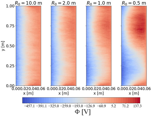
Starting from an equal density of ions and electrons in the same positions at the initial stage, they relocate their positions in time. The electron and ion densities in the upper and lower regions will not be in balance with each other, with an increase in the running time. Under the strong grad-B drift, the electron density is high in the lower region and low in the upper, which is the opposite of the ion density. Therefore, the electron density is higher than the ion density in the lower region, and vice versa. Ion and electron fluxes are locally different, and the electric field is self-consistently induced. The electrical potential is formed inside the simulation box and is different between the upper and lower regions due to a different distribution of particle densities. Figure 4 shows the potential profile in the simulation box with the various major radii. At the limiter and at $x=L_x$, particles are fully absorbed. Once a particle is lost at the limiter, a new particle is injected into the simulation in the closed magnetic field region where $x<x_{\text{w}}$. The number of electron loss is larger than the ion loss in the limiter leads to more number of electrons are injected in the closed magnetic field regions than the ions. Subsequently, the potential in this region will have the negative values. Once the simulation reaches the equilibrium stage, the number of lost electrons is nearly equal to that of ions. The number of ions remaining in front of the limiter is higher than the electrons. Consequently, the potential profile near the limiter in the poloidal direction will have higher positive values than other regions. The potential profile is almost symmetric along the $y$ direction in a case when the large major radius is used. The potential profile breaks its symmetrical structure for a smaller major radius system, causing differences between the upper and lower regions. To explain the occurrence of the asymmetric potential profile, we examine the particle density figures, Figure 3. In the case of a large major radius system, the difference between electron and ion densities in each region is not obvious. The loss of electrons and ions along the left boundary is comparable. Electron and ion densities are nearly equal in each region. The formation of the potential profile is similar between the upper and the lower regions. When a low major radius is added, as discussed, the difference between the electron and ion densities (i.e., $\mathrm{\Delta }n=n_e-n_i$) has an opposite sign for each region. This value affects that of the Laplacian of the potential given in Equation 4. The Laplacian will have the opposite signs for the upper and lower regions. Consequently, the formation of the potential structure in these two regions is dissimilar. The asymmetry of the potential profile appears when strong toroidicity is applied. In order words, the asymmetry potential depends on the strength of the grad-B drift. The potential will get a clearer asymmetric figure if the torus has a stronger toroidicity. This dependency can be easily captured in the PIC simulation rather than using a fluid model because the PIC model can explicitly include the drift effects. PIC simulation is a powerful tool to study the drift effect and particle motion compared to the other models. Another phenomenon that can be obtained while studying the potential formation in the axisymmetric magnetic field is the effects of the finite Larmor radius. Because PIC simulation can chase the gyro motion of the particles in each time step, the influence of the Larmor radius on particle motion can be captured by using PIC simulation (see Supplementary Appendix S1).

Figure 4

Figure 4. The electrical potential is self-consistently formed in the simulation. The potential is symmetric in the large major radius system from the mid-line $y=L_y/2$. The potential breaks the symmetric structure to become an asymmetric behavior when the system has a smaller major radius.

4 Discussion

The effects of the grad-B drift on particle motion and potential formation are studied using PIC simulation. We model a region near the LCFS in the toroidal limiter by transferring the torus geometry into two-dimensional slab geometry. The magnetic field is fixed in time and includes the curvature and toroidal gradient. The simulation is set up to be symmetrical along the y direction via the mid-line $y=L_y/2$. The asymmetry of the potential profile has been found to be dependent on the toroidal gradient of the magnetic field. When increasing the major radius of the torus, the magnetic field has a stronger toroidal gradient for a fixed minor radius. The strong grad-B drift increases the particle transport in the radial direction and forces more particles to be lost at the boundary. The electrons and ions spiral contrariwise. Moreover, the grad-B drift is the opposite for ions and electrons. Therefore, the movements of the electrons and ions under the grad-B drift are inverse. An imbalance of the electron and ion densities in these regions will break the symmetric structure of the potential. The electrical potential becomes asymmetric when the toroidicity of the torus is strong. The PIC simulation can capture all effects generated from the drifts, computing the self-consistently formed potential. This property helps the PIC simulation become a powerful model for numerical studies of particle transport and drift effects, even though it consumes much time and requires a huge memory. The optimization and parallelization processes for the PIC code still need to be improved for studying a large-scale and complicated system. There will be a perspective picture for including a three-dimensional magnetic field structure to study the potential formation, similar to realistic tokamak devices using the PIC code. This will be in our future work.

Data availability statement

The raw data supporting the conclusions of this article will be made available by the authors, without undue reservation.

Author contributions

TL: Writing–original draft. YS: Writing–review and editing. HO: Writing–review and editing. HH: Writing–review and editing. TM: Writing–review and editing.

Funding

The author(s) declare that financial support was received for the research, authorship, and/or publication of this article. This work was performed on the “Plasma Simulator” (NEC SX-Aurora TSUBASA) of NIFS with the support and under the auspices of the NIFS Collaboration Research program (NIFS21KNST189 and NIFS22KISS005). This work was partially supported by “PLADyS,” JSPS Core-to-Core Program, A. Advanced Research Network.

Conflict of interest

The authors declare that the research was conducted in the absence of any commercial or financial relationships that could be construed as a potential conflict of interest.

Publisher’s note

All claims expressed in this article are solely those of the authors and do not necessarily represent those of their affiliated organizations, or those of the publisher, the editors and the reviewers. Any product that may be evaluated in this article, or claim that may be made by its manufacturer, is not guaranteed or endorsed by the publisher.

References

1. Freidberg JP. Plasma physics and fusion energy. Cambridge: Cambridge University Press (2008).

Google Scholar

2. Kamiya K, Ida K, Yoshinuma M, Suzuki C, Suzuki Y, Yokoyama M, et al. Characterization of edge radial electric field structures in the large helical device and their viability for determining the location of the plasma boundary. Nucl Fusion (2012) 53:013003. doi:10.1088/0029-5515/53/1/013003

CrossRef Full Text | Google Scholar

3. De Aguilera AM, Castejón F, Ascasíbar E, Blanco E, De la Cal E, Hidalgo C, et al. Magnetic well scan and confinement in the tj-ii stellarator. Nucl Fusion (2015) 55:113014. doi:10.1088/0029-5515/55/11/113014

CrossRef Full Text | Google Scholar

4. Suzuki Y, Ida K, Kamiya K, Yoshinuma M, Sakakibara S, Watanabe K, et al. 3d plasma response to the magnetic field structure in the large helical device. Nucl Fusion (2013) 53:073045. doi:10.1088/0029-5515/53/7/073045

CrossRef Full Text | Google Scholar

5. Suzuki Y, Ida K, Kamiya K, Yoshinuma M, Tsuchiya H, Inagaki S, et al. Investigation of radial electric field in the edge region and magnetic field structure in the large helical device. Plasma Phys Controlled Fusion (2013) 55:124042. doi:10.1088/0741-3335/55/12/124042

CrossRef Full Text | Google Scholar

6. Rozhansky V, Kaveeva E, Molchanov P, Veselova I, Voskoboynikov S, Coster D, et al. Modification of the edge transport barrier by resonant magnetic perturbations. Nucl fusion (2010) 50:034005. doi:10.1088/0029-5515/50/3/034005

CrossRef Full Text | Google Scholar

7. Rozhansky V. Drifts, currents, and radial electric field in the edge plasma with impact on pedestal, divertor asymmetry and rmp consequences. Contrib Plasma Phys (2014) 54:508–16. doi:10.1002/ctpp.201410011

CrossRef Full Text | Google Scholar

8. Birdsall CK, Langdon AB. Plasma physics via computer simulation. Boca Raton, Florida: CRC Press (2004).

Google Scholar

9. Stacey W. Extensions of ion orbit loss theory. Phys Plasmas (2014) 21:014502. doi:10.1063/1.4861612

CrossRef Full Text | Google Scholar

10. Tskhakaya D, Matyash K, Schneider R, Taccogna F. The particle-in-cell method. Contrib Plasma Phys (2007) 47:563–94. doi:10.1002/ctpp.200710072

CrossRef Full Text | Google Scholar

11. Stangeby PC. The plasma boundary of magnetic fusion devices, 224. Philadelphia, Pennsylvania: Institute of Physics Pub (2000). doi:10.1201/9780367801489

CrossRef Full Text | Google Scholar

12. Stangeby P, McCracken G. Plasma boundary phenomena in tokamaks. Nucl Fusion (1990) 30:1225–379. doi:10.1088/0029-5515/30/7/005

CrossRef Full Text | Google Scholar

13. Nanbu K. Theory of cumulative small-angle collisions in plasmas. Phys Rev E (1997) 55:4642–52. doi:10.1103/physreve.55.4642

CrossRef Full Text | Google Scholar

14. Nanbu K, Yonemura S. Weighted particles in coulomb collision simulations based on the theory of a cumulative scattering angle. J Comput Phys (1998) 145:639–54. doi:10.1006/jcph.1998.6049

CrossRef Full Text | Google Scholar

15. Leonard AW. Edge-localized-modes in tokamaks. Phys Plasmas (2014) 21:090501. doi:10.1063/1.4894742

CrossRef Full Text | Google Scholar

16. Ida K, Hidekuma S, Miura Y, Fujita T, Mori M, Hoshino K, et al. Edge electric-field profiles of h-mode plasmas in the jft-2m tokamak. Phys Rev Lett (1990) 65:1364–7. doi:10.1103/physrevlett.65.1364

PubMed Abstract | CrossRef Full Text | Google Scholar

17. Liang Y, Koslowski H, Thomas P, Nardon E, Alper B, Andrew P, et al. Active control of type-i edge-localized modes with n= 1 perturbation fields in the jet tokamak. Phys Rev Lett (2007) 98:265004. doi:10.1103/physrevlett.98.265004

PubMed Abstract | CrossRef Full Text | Google Scholar

18. Kirk A, Wilson H, Counsell G, Akers R, Arends E, Cowley S, et al. Spatial and temporal structure of edge-localized modes. Phys Rev Lett (2004) 92:245002. doi:10.1103/physrevlett.92.245002

PubMed Abstract | CrossRef Full Text | Google Scholar

19. Nunes I, Conway G, Loarte A, Manso M, Serra F, Suttrop W, et al. Characterization of the density profile collapse of type i elms in asdex upgrade with high temporal and spatial resolution reflectometry. Nucl fusion (2004) 44:883–91. doi:10.1088/0029-5515/44/8/007

CrossRef Full Text | Google Scholar

20. Derouillat J, Beck A, Pérez F, Vinci T, Chiaramello M, Grassi A, et al. Smilei: a collaborative, open-source, multi-purpose particle-in-cell code for plasma simulation. Computer Phys Commun (2018) 222:351–73. doi:10.1016/j.cpc.2017.09.024

CrossRef Full Text | Google Scholar

21. Miyamoto K. Fundamentals of plasma physics and controlled fusion (iwanami book service center tokyo) (1997).

Google Scholar

22. Ghendrih P, Cartier-Michaud T, Dif-Pradalier G, Esteve D, Garbet X, Grandgirard V, et al. Collisions in magnetised plasmas. ESAIM: Proc Surv (2015) 50:81–112. doi:10.1051/proc/201550005

CrossRef Full Text | Google Scholar

23. Chen FF. Introduction to plasma physics and controlled fusion, 1. Springer (1984). doi:10.1007/978-3-319-22309-4

CrossRef Full Text | Google Scholar