Bifurcation analysis of a Leslie-type predator–prey system with prey harvesting and group defense

In this paper, we investigate a Leslie-type predator–prey model that incorporates prey harvesting and group defense, leading to a modified functional response. Our analysis focuses on the existence and stability of the system’s equilibria, which are essential for the coexistence of predator and prey populations and the maintenance of ecological balance. We identify the maximum sustainable yield, a critical factor for achieving this balance. Through a thorough examination of positive equilibrium stability, we determine the conditions and initial values that promote the survival of both species. We delve into the system’s dynamics by analyzing saddle-node and Hopf bifurcations, which are crucial for understanding the system transitions between various states. To evaluate the stability of the Hopf bifurcation, we calculate the first Lyapunov exponent and offer a quantitative assessment of the system’s stability. Furthermore, we explore the Bogdanov–Takens (BT) bifurcation, a co-dimension 2 scenario, by employing a universal unfolding technique near the cusp point. This method simplifies the complex dynamics and reveals the conditions that trigger such bifurcations. To substantiate our theoretical findings, we conduct numerical simulations, which serve as a practical validation of the model predictions. These simulations not only confirm the theoretical results but also showcase the potential of the model for predicting real-world ecological scenarios. This in-depth analysis contributes to a nuanced understanding of the dynamics within predator–prey interactions and advances the field of ecological modeling.

1 Introduction

Since the pioneering work of Lotka and Volterra, who introduced a pair of differential equations to describe predator–prey dynamics, predator–prey models have attracted considerable interest from both mathematicians and biologists due to their widespread applicability [1]. Predominantly, predator–prey models have been developed around two main scenarios: (i) the growth function of the predator is directly proportional to its predation function, capturing the functional response of predators to prey availability, and (ii) the growth function of the predator is decoupled from its predation function, suggesting a more intricate relationship between the predator and prey.

Moreover, the growth term of the predator in these models is often portrayed as a function that depends not only on prey density but also on the predator-to-prey ratio, adding another dimension of complexity to the interactions. Among these diverse models, the Leslie-type model has emerged as a particularly influential paradigm. Its sophisticated treatment of predator–prey interactions has solidified its role as a fundamental framework in ecological studies, aiding in the comprehension of the delicate equilibrium within ecosystems.

[2] proposed a Leslie-type model to describe the relationship between predators and their prey:

$\begin{array}{cc}\hfill \frac{\mathrm{d}x}{\mathrm{d}t}& =rx\left(1-\frac{x}{K}\right)-yf\left(x\right),\hfill \\ \hfill \frac{\mathrm{d}y}{\mathrm{d}t}& =qy\left(1-\frac{y}{px}\right),\hfill \end{array}$

where x and y denote the population densities of the prey and predators, respectively. In the absence of predators, the growth of prey populations is commonly modeled using a logistic growth function, characterized by an intrinsic growth rate r and an environmental carrying capacity K. This model assumes that population growth is limited by the availability of resources as the population size approaches the carrying capacity. The functional response, represented by f(x), describes how the rate of prey consumption by predators varies with the density of the prey population. In contrast, the growth rate of the predator is a Leslie-type growth function expressed as $q\left(1-\frac{y}{px}\right)$, which depends on both the prey density and the predator density. Here, q denotes the intrinsic per capita growth rate of the predator in the presence of abundant prey, p is a scaling factor that relates the carrying capacity of the predator to that of the prey, and the term $1-\frac{y}{px}$ reflects the diminishing growth rate as the predator-to-prey ratio approaches one, indicating prey scarcity. This growth function is particularly useful for simulating systems where the success of the predator in capturing the prey is influenced not only by prey abundance but also by the density of the predator population. It captures the competitive pressures and the complex dynamics of resource allocation within an ecosystem, offering a more nuanced understanding of predator–prey interactions. The functional response function f(x) is typically categorized into four classical types: Holling type I [3], Holling type II [4], Holling type III [5, 6], and Holling type IV [7, 8]. These types are defined by specific mathematical expressions that reflect different assumptions about predator behavior and the efficiency of predation. Most predator–prey models incorporate one of these functional responses or their modifications.

Recently, [9, 10] proposed a novel functional response model that replaces the traditional prey density with the square root of prey density in the context of the Holling type II functional response. This innovation is particularly pertinent for prey species that exhibit herding behavior, where only peripheral individuals engage with predators. This revised functional response more accurately reflects how the protective effects of group living affect the rate at which predators encounter and consume the prey. Combining their functional response functions, we propose the following Leslie-type model:

$\begin{array}{cc}\hfill \frac{\mathrm{d}x}{\mathrm{d}t}& =rx\left(1-\frac{x}{K}\right)-\frac{\alpha \sqrt{x}y}{1+T_h\alpha \sqrt{x}},\hfill \\ \hfill \frac{\mathrm{d}y}{\mathrm{d}t}& =qy\left(1-\frac{y}{px}\right),\hfill \end{array}(1)$

where α presents the search efficiency of the predator for the prey and T_h denotes the average handing time for each prey.

Before going into details, by substituting

$\bar{x}=\frac{x}{K},\bar{y}=\frac{\alpha y}{r\sqrt{K}},\bar{t}=rt,a=T_h\alpha \sqrt{K},b=\frac{q}{r},d=\frac{r}{p\alpha \sqrt{K}},$

into model Eq. 1 and dropping the bars, we obtain

$\begin{array}{cc}\hfill \frac{\mathrm{d}x}{\mathrm{d}t}& =x\left(1-x\right)-\frac{\sqrt{x}y}{1+a\sqrt{x}},\hfill \\ \hfill \frac{\mathrm{d}y}{\mathrm{d}t}& =by\left(1-d\frac{y}{x}\right).\hfill \end{array}(2)$

Over the past three decades, a considerable amount of research has been devoted to understanding the effects of harvesting on the dynamics of predator–prey systems and its implications for the management of renewable resources. [11] explored a predator–prey model that includes Michaelis–Menten-type predator harvesting. In a similar vein, [12] discussed a modified Leslie–Gower model incorporating Michaelis–Menten-type prey harvesting. [13] investigated a model where both predator and prey populations exhibit logistic growth and are subject to nonlinear harvesting. The impact of proportional harvesting on the dynamic behavior of predator–prey models was examined by [14, 15]. [16] provided a detailed bifurcation analysis for a model with Holling-type II functional response and a constant harvesting rate. [17] also studied a model with constant prey harvesting. [18, 19] studied the dynamic behaviors of the predator–prey systems with a Holling- and Leslie-type or Leslie–Gower model with constant-yield prey harvesting, revealing a diverse array of bifurcations. [20] and [21] discussed ratio-dependent predator–prey systems with constant harvesting for both prey and predators, respectively. [22] investigated a system where the prey population forms herds as a defense against predators, and both species are exposed to a constant harvesting rate.

Inspired by these studies, we introduce the impact of a constant harvesting rate for the prey into Eq. 2 and obtain the following results:

$\begin{array}{cc}\hfill \frac{\mathrm{d}x}{\mathrm{d}t}& =x\left(1-x\right)-\frac{\sqrt{x}y}{1+a\sqrt{x}}-h,\hfill \\ \hfill \frac{\mathrm{d}y}{\mathrm{d}t}& =by\left(1-d\frac{y}{x}\right),\hfill \end{array}(3)$

where h represents the rate of prey harvesting.

It should be noted that system Eq. 2 is a Leslie-type predator–prey model that incorporates prey group defense mechanisms. Furthermore, system Eq. 3 extends this framework by accounting for the constant harvesting of the prey within system Eq. 2. To date, the dynamic behaviors of both systems Eq. 2 and Eq. 3 remain unexplored. Given the significance of biological resources as a sustainable source for human utilization and considering the rapid industrialization and population growth that have led to an inevitable increase in the utilization of various biological assets, it is imperative to investigate the impact of harvesting behavior on the population of both the predator and prey, particularly when prey group defense is involved, for the sake of maintaining ecological balance. In this paper, we study the dynamic behaviors of these two systems. Through rigorous mathematical analysis, we find that the population of the prey will be sustained without the effect of prey harvesting. However, due to the emergence of prey harvesting, system Eq. 3 exhibits complex dynamic behaviors and undergoes saddle-node, Hopf, and Bogdanov–Takens (BT) bifurcations. System Eq. 3 has bi-stable behavior due to saddle-node bifurcation, and whether the prey becomes extinct or not depends on the prey harvesting intensity. Specifically, we determine the maximum sustainable yield as $h_{\mathit{MSY}}=\frac{1}{4}$. Once the prey harvesting rate h exceeds h_MSY, both the prey and predator species face extinction. This insight underscores the importance of selecting an appropriate harvesting rate, specifically to ensure the co-existence of the predator and prey, thereby sustaining ecological balance.

The structure of this paper is shown in Figure 1. Section 2 discusses the existence and stability of the equilibria for system Eq. 2. Section 3 delves into the investigation of the equilibria for system Eq. 3, providing both analytical insights and corroborating numerical results. Section 4 focuses on the bifurcation analysis of system Eq. 3, examining both saddle-node and Hopf bifurcations. Additionally, this section explores the Bogdanov–Takens bifurcation within the same system. Concluding remarks are given in Section 5, summarizing the key findings and implications of the study.

Figure 1

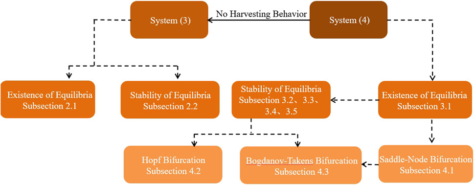
Figure 1. Flowchart of studies of the prey–predator system focusing on the harvesting setting in this paper.

2 Equilibria of system (3)

2.1 Existence of equilibria

To determine the equilibria of system Eq. 2, we analyze the prey and predator nullclines, which are given by the following equations:

$\begin{array}{cc}\hfill x\left(1-x\right)-\frac{\sqrt{x}y}{1+a\sqrt{x}}& =0,\hfill \\ \hfill by\left(1-d\frac{y}{x}\right)& =0.\hfill \end{array}$

From these nullclines, it is evident that system Eq. 2 has a unique boundary equilibrium at $E_0^0=(\mathrm{1,0})$. To identify potential positive equilibria, we solve the following equations:

$\begin{array}{cc}\hfill f\left(x\right)& ≔1-x-\frac{\sqrt{x}}{d\left(1+a\sqrt{x}\right)}=0,\hfill \\ \hfill y& ≔\frac{x}{d}.\hfill \end{array}$

By substituting $\sqrt{x}=z$, we transform the problem of finding positive solutions to f(x) = 0 into finding positive solutions to g(z) = adz³ + dz² + (1 − ad)z − d = 0. Through algebraic analysis, we can easily determine that g(z) = 0 has a unique positive solution. Consequently, system Eq. 2 has a unique positive equilibrium point, denoted as $E_0^{*}=(x_0^{*},y_0^{*})$, where $y_0^{*}=\frac{x_0^{*}}{d}$, $x_0^{*}=z_0^2$, and z₀ is the unique positive root of g(z) = 0. Based on this analysis, we can formulate the following theorem regarding the number of equilibria in system Eq. 2.

Theorem 2.1. System Eq. 2 possesses a unique boundary equilibrium $E_0^0=(\mathrm{1,0})$ and unique positive equilibrium denoted by $E_0^{*}=(x_0^{*},y_0^{*})$.

2.2 Stability of equilibria

Theorem 2.2. For all positive parameters, system Eq. 2 has a boundary equilibrium $E_0^0$ and a positive equilibrium $E_0^{*}$. Moreover, the boundary equilibrium $E_0^0$ is always a hyperbolic saddle. Furthermore, the positive equilibrium $E_0^{*}$ is a sink when b > b₀, a source when b < b₀, or a center when b = b₀, where $b_0=1-z_0^2-\frac{z_0}{2d{(1+a{z}_0)}^2}$ and z₀ is the positive root of g(z) = 0.

Proof. The Jacobian matrix of system Eq. 2 evaluated at $E_0^0$ is given by

$J\left(E_0^0\right)=\left(\begin{array}{cc}\hfill -1\hfill & \hfill -\frac{1}{1+a}\hfill \\ \hfill 0\hfill & \hfill b\hfill \end{array}\right).$

It is obvious that the matrix $J(E_0^0)$ has a positive eigenvalue b and a negative eigenvalue −1. Therefore, $E_0^0$ is always a hyperbolic saddle.

The Jacobian matrix of system Eq. 2 evaluated at $E_0^{*}$ is given by

$J\left(E_0^{*}\right)=\left(\begin{array}{cc}\hfill 1-2x_0^{*}-\frac{\sqrt{x_0^{*}}}{2d{\left(1+a\sqrt{x_0^{*}}\right)}^2}\hfill & \hfill -\frac{\sqrt{x_0^{*}}}{1+a\sqrt{x_0^{*}}}\hfill \\ \hfill \frac{b}{d}\hfill & \hfill -b\hfill \end{array}\right)=\left(\begin{array}{cc}\hfill 1-2z_0^2-\frac{z_0}{2d{\left(1+a{z}_0\right)}^2}\hfill & \hfill -\frac{z_0}{1+a{z}_0}\hfill \\ \hfill \frac{b}{d}\hfill & \hfill -b\hfill \end{array}\right).$

According to g(z₀) = 0, we can obtain $1-z_0^2=\frac{z_0}{d(1+a{z}_0)}$. Then,

$\begin{array}{ccc}\hfill Det\left[J\left(E_0^{*}\right)\right]& =\hfill & b{z}_0^2+\frac{b{z}_0}{2d{\left(1+a{z}_0\right)}^2}>0,\hfill \\ \hfill Tr\left[J\left(E_0^{*}\right)\right]& =\hfill & 1-z_0^2-\frac{z_0}{2d{\left(1+a{z}_0\right)}^2}-b\triangleq b_0-b.\hfill \end{array}$

Hence, when b > b₀, $Tr[J(E_0^{*})]<0$, the matrix $J(E_0^{*})$ has two negative part eigenvalues, and $E_0^{*}$ is a sink. When b < b₀, then $Tr[J(E_0^{*})]>0$, the matrix $J(E_0^{*})$ has two positive part eigenvalues, and $E_0^{*}$ is a source. When b = b₀, then $Tr[J(E_0^{*})]=0$, the matrix $J(E_0^{*})$ has a pair of purely imaginary eigenvalues, and $E_0^{*}$ is a center.

3 Equilibria of system (4)

3.1 Existence of equilibria

This section conducts a qualitative analysis of model Eq. 3. With the biological context in mind, we focus on examining the dynamics of system Eq. 3 within the closed first quadrant, denoted as $R_{+}^2$, in the (x, y) coordinate plane.

In order to obtain the equilibria of system Eq. 3, we first study the roots of the following equations:

$\begin{array}{cc}\hfill x\left(1-x\right)-\frac{\sqrt{x}y}{1+a\sqrt{x}}-h=0,& \hfill \\ \hfill by\left(1-d\frac{y}{x}\right)=0.\end{array}(4)$

Regarding the count of boundary equilibria for system Eq. 3, we derived the subsequent theorem.

Theorem 3.1. (i) When $h=\frac{1}{4}$, system Eq. 3 admits a unique boundary equilibrium $E_0=(\frac{1}{2},0)$.

(ii) When $0<h<\frac{1}{4}$, system Eq. 3 admits two boundary equilibria E_i = (x_i, 0) (i = 1, 2), where $x_1=\frac{1-\sqrt{1-4h}}{2}$ and $x_2=\frac{1+\sqrt{1-4h}}{2}$.

Proof. When h exceeds $\frac{1}{4}$, $\dot{x}=x(1-x)-h-\frac{\sqrt{x}y}{1+a\sqrt{x}}<0$. This implies that the dynamics of system Eq. 3 within $R_{+}^2$ are inherently trivial. Consequently, the prey species faces extinction, an event that subsequently triggers the extinction of the predator. It is evident that system Eq. 3 lacks any equilibrium points within the positive quadrant $R_{+}^2$.

We next explore the existence of boundary equilibria under the condition that $h\le \frac{1}{4}$. Specifically, when y = 0 in Eq. 4, we are confronted with the following equation:

$x^2-x-h=0.(5)$

It is straightforward to determine that when $h<\frac{1}{4}$, Eq. 5 has two distinct roots, denoted as x₁ and x₂. Conversely, when $h=\frac{1}{4}$, the equation yields a unique root, which is $\frac{1}{2}$.

Note that

$\begin{array}{cc}\hfill f_1\left(z\right)& \triangleq ad{z}^5+d{z}^4+\left(1-ad\right)z^3-d{z}^2+adhz+hd,\hfill \\ \hfill g_1\left(z\right)& \triangleq f_1^{\prime }\left(z\right)=5ad{z}^4+4d{z}^3+3\left(1-ad\right)z^2-2dz+adh,\hfill \\ \hfill h_1\left(z\right)& \triangleq g_1^{\prime }\left(z\right)=20ad{z}^3+12d{z}^2+6\left(1-ad\right)z-2d.\hfill \end{array}(6)$

Regarding the positive equilibria of system Eq. 3, we have the following theorem.

Theorem 3.2. (i) When $h=h_2^{*}$ and $h_2^{*}<h_1^{*}$, system Eq. 3 has a unique positive equilibrium E₃ = (x₃, y₃).

(ii) When $h<\min \{h_1^{*},h_2^{*}\}$, system (4) has two different positive equilibria E_i = (x_i, y_i) (i = 4, 5),

where $h_1^{*}=\frac{5a{z}_1^4+2z_1^3+z_1}{a}$, $h_2^{*}=\frac{z_3^2(2a{z}_3^3+z_3^2+1)}{2a{z}_3+3}$, z₃ is the larger positive root between two positive roots of g₁(z) = 0, and z₁ is the only positive root of h₁(z) = 0.

Proof. When y ≠ 0, then $y=\frac{x}{d}$ according to Eq. 5, and x is the positive root of the equation

$x\left(1-x\right)\left(1+a\sqrt{x}\right)d-x\sqrt{x}-dh\left(1+a\sqrt{x}\right)=f_1\left(z\right),$

where $z=\sqrt{x}$ and f₁(z) is given in Eq. 6.

Through algebraic analysis, we find that the equation h₁(z) = 0 has a unique positive root, denoted as z₁. When g₁(z₁) < 0, which corresponds to $h<h_1^{*}\triangleq \frac{5a{z}_1^4+2z_1^3+z_1}{a}$, the equation g₁(z) = 0 admits two distinct positive roots, z₂ and z₃ (with z₂ < z₃). If f₁(z₃) = 0, which occurs when $h=h_2^{*}\triangleq \frac{z_3^2(2a{z}_3^3+z_3^2+1)}{2a{z}_3+3}$, then the equation f₁(z) = 0 has a unique positive root. Consequently, system Eq. 3 admits a unique positive equilibrium E₃ = (x₃, y₃), where $x_3=z_3^2$ and $y_3=\frac{x_3}{d}$. If f₁(z₃) < 0, corresponding to $h<h_2^{*}$, then the equation f₁(z) = 0 has two distinct positive roots, z₄ and z₅ (with z₂ < z₄ < z₃ < z₅). In this case, system Eq. 3 has two distinct positive equilibria, E₄ = (x₄, y₄) and E₅ = (x₅, y₅), where $x_4=z_4^2$, $x_5=z_5^2$, $y_4=\frac{x_4}{d}$, and $y_5=\frac{x_5}{d}$.

3.2 Stability of equilibrium E₀

Theorem 3.3. When $h=\frac{1}{4}$, system Eq. 3 possesses a unique boundary equilibrium at $E_0=(\frac{1}{2},0)$, which is classified as a saddle-node. This equilibrium divides a sufficiently small neighborhood into two parts, separated by two separatrices that approach E₀ from above and below. One part forms a parabolic sector, while the other comprises two hyperbolic sectors. Additionally, the parabolic sector is situated in the left half-plane, and the equilibrium E₀ acts as a repelling saddle-node. The dynamics of the system in this scenario are illustrated in the phase portraits shown in Figure 2A.

Figure 2

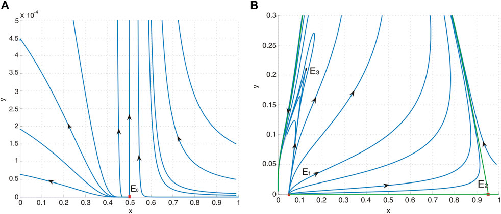
Figure 2. (A) Phase portrait of system (4) with a = 0.4, b = 0.5, d = 0.6, and $h=\frac{1}{4}$. (B) Phase portrait of system (4) with a = 0.4, b = 0.5193087015, d = 0.6, and h = 0.04485055324. E₁ is an unstable node, E₂ is a saddle, and E₃ is a cusp.

Proof. The Jacobian matrix J(E₀) of system Eq. 3 evaluated at E₀ is

$J\left(E_0\right)=\left(\begin{array}{cc}\hfill 0\hfill & \hfill -\frac{1}{\sqrt{2}+a}\hfill \\ \hfill 0\hfill & \hfill b\hfill \end{array}\right).$

Given that Det[J(E₀)] = 0, we can conclude that the equilibrium $(\frac{1}{2},0)$ is nonhyperbolic, indicating that it is a degenerate equilibrium. It is evident that the eigenvalues of the Jacobian matrix J(E₀) are λ₁ = 0 and λ₂ = b. To ascertain the stability of E₀, we perform a transformation by shifting the equilibrium to the origin using the transformation $(X,Y)=(x-\frac{1}{2},y)$. We then expand system Eq. 3 in a power series up to the second order around the origin. Under this transformation, system Eq. 3 becomes

$\begin{array}{cc}\hfill \dot{X}& =-\frac{1}{\sqrt{2}+a}Y-X^2-\frac{\sqrt{2}}{{\left(\sqrt{2}+a\right)}^2}XY+P_1\left(X,Y\right),\hfill \\ \hfill \dot{Y}& =bY-2bd{Y}^2+Q_1\left(X,Y\right),\hfill \end{array}$

where P₁(X, Y) and Q₁(X, Y) are smooth functions of at least the third order with respect to (X, Y).

Then, making the transformation

$\left(\begin{array}{c}\hfill X\hfill \\ \hfill Y\hfill \end{array}\right)=\left(\begin{array}{cc}\hfill 1\hfill & \hfill -\frac{1}{\sqrt{2}+a}\hfill \\ \hfill 0\hfill & \hfill b\hfill \end{array}\right)\left(\begin{array}{c}\hfill x\hfill \\ \hfill y\hfill \end{array}\right),$

and introducing a new time variable τ = bt, for which we retain t to denote τ for notational simplicity, we obtain

$\begin{array}{cc}\hfill \dot{x}& =a_{20}{x}^2+a_{11}xy+a_{02}{y}^2+P_2\left(x,y\right),\hfill \\ \hfill \dot{y}& =y-2bd{y}^2+Q_2\left(x,y\right),\hfill \end{array}$

where P₂(x, y) and Q₂(x, y) are smooth functions of at least the third order with respect to (x, y) and

$\begin{array}{cc}\hfill a_{20}& =-\frac{a^5+5\sqrt{2}{a}^4+20a^3+20\sqrt{2}{a}^2+20a+4\sqrt{2}}{{\left(a+\sqrt{2}\right)}^{5}b}<0,\hfill \\ \hfill a_{11}& =\frac{2a^4-\sqrt{2}\left(b+8\right)a^3+6\left(4-b\right)a^2-2\sqrt{2}\left(3b-8\right)a+4\left(2-b\right)}{{\left(a+\sqrt{2}\right)}^{5}b},\hfill \\ \hfill a_{02}& =\frac{2a^2{b}^{2}d\left(a^2+4\sqrt{2}a+12\right)+a^2\left(a-\sqrt{2}b+3\sqrt{2}\right)+a\left(16b^{2}d+6-4b\right)+8b^{2}d-2\sqrt{2}b+2\sqrt{2}}{{\left(a+\sqrt{2}\right)}^{5}b}.\hfill \end{array}$

According to Theorem 7.1 from Chapter 2 in [23], the equilibrium E₀ is classified as a saddle-node. This implies that the vicinity of E₀ is bifurcated by two separatrices that approach E₀ from above and below. One region forms a parabolic sector, while the other comprises two hyperbolic sectors. Additionally, the parabolic sector is situated in the right half-plane, and E₀ acts as a repelling saddle-node.

3.3 Stability of equilibria E₁ and E₂

Theorem 3.4. When $0<h<\frac{1}{4}$, system Eq. 3 has two different boundary equilibria E₁ and E₂. Moreover, E₁ is always a hyperbolic unstable node, and E₂ is always a hyperbolic saddle. The corresponding phase portraits are shown in Figure 2B and Figure 3.

Figure 3

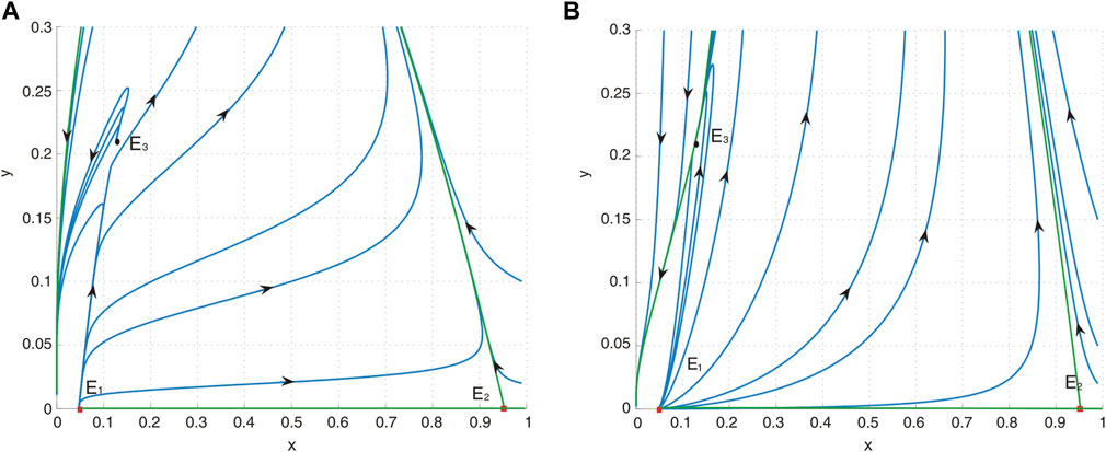
Figure 3. (A) Phase portrait of system (4) with a = 0.4, b = 0.2, d = 0.6, and h = 0.04485055324. E₁ is an unstable node, E₂ is a saddle, and E₃ is a repelling saddle node. (B) Phase portrait of system (4) with a = 0.4, b = 1.2, d = 0.6, and h = 0.04485055324. E₁ is an unstable node, E₂ is a saddle, and E₃ is an attracting saddle node.

Proof. The Jacobian matrix J(E₁) of system Eq. 3 evaluated at E₁ is

$J\left(E_1\right)=\left(\begin{array}{cc}\hfill \sqrt{1-4h}\hfill & \hfill -\frac{\sqrt{x_1}}{1+a\sqrt{x_1}}\hfill \\ \hfill 0\hfill & \hfill b\hfill \end{array}\right).$

We can obtain that the eigenvalues are ${\lambda }_1=\sqrt{1-4h}>0$ and λ₂ = b > 0. Hence, E₁ is a hyperbolic unstable node.

The Jacobian matrix J(E₂) of system Eq. 3 evaluated at E₂ is

$J\left(E_2\right)=\left(\begin{array}{cc}\hfill -\sqrt{1-4h}\hfill & \hfill -\frac{\sqrt{x_2}}{1+a\sqrt{x_2}}\hfill \\ \hfill 0\hfill & \hfill b\hfill \end{array}\right).$

It is easy to observe that the eigenvalues are ${\lambda }_1=-\sqrt{1-4h}<0$ and λ₂ = b > 0. Hence, E₂ is a hyperbolic saddle.

3.4 Stability of equilibrium E₃

Now, we investigate the stability of equilibrium E₃. The Jacobian matrix J(E₃) of system Eq. 3 evaluated at E₃ is

$J\left(E_3\right)=\left(\begin{array}{cc}\hfill 1-2x_3-\frac{\sqrt{x_3}}{2d{\left(1+a\sqrt{x_3}\right)}^2}\hfill & \hfill -\frac{\sqrt{x_3}}{1+a\sqrt{x_3}}\hfill \\ \hfill \frac{b}{d}\hfill & \hfill -b\hfill \end{array}\right)\triangleq \left(\begin{array}{cc}\hfill a_{10}\hfill & \hfill a_{01}\hfill \\ \hfill b_{10}\hfill & \hfill b_{01}\hfill \end{array}\right).$

Straightforward computation shows that, due to $x_3=z_3^2$,

$Det\left[J\left(E_3\right)\right]=\frac{b}{2d{\left(1+a{z}_3\right)}^2}l\left(z_3\right),$

where

$l\left(z\right)=4a^{2}d{z}^4+8ad{z}^3+\left(2a+4d-2a^{2}d\right)z^2+\left(3-4ad\right)z-2d.$

Since f(z₃) = 0, from Theorem 3.2, we can obtain

$h=-\frac{z_3^2\left(ad{z}_3^3+d{z}_3^2+\left(1-ad\right)z_3-d\right)}{d\left(1+a{z}_3\right)}.$

Substituting g₁(z₃) in the above equation yields $g_1(z_3)=\frac{z_3}{1+a{z}_3}l(z_3)$. Because z₃ is a positive root of g₁(z) = 0, g₁(z₃) = 0 and l(z₃) = 0. Therefore, Det[J(E₃)] = 0. Therefore, we can establish that equilibrium E₃ is nonhyperbolic, which means it is a degenerate equilibrium. To elaborate further, we present the following theorem:

Theorem 3.5. (i) If $a_{10}+b_{01}\ne 0\left(b\ne b_1^{*}\triangleq 1-2x_3-\frac{\sqrt{x_3}}{2d{(1+a\sqrt{x_3})}^2}\right)$,

(i-1) $a_{10}+b_{01}<0(b>b_1^{*})$, then the parabolic sector is located in the right half-plane, and E₃ is an attracting saddle-node. The corresponding phase portrait is shown in Figure 3B.

(i-2) $a_{10}+b_{01}>0(b<b_1^{*})$, then the parabolic sector is located in the left half-plane, and E₃ is a repelling saddle-node. The corresponding phase portrait is shown in Figure 3A.

(ii) When $a_{10}+b_{01}=0(b=b_1^{*})$, E₃ represents a degenerate critical point, specifically a cusp. Furthermore, E₃ is a cusp of co-dimension 2 under the condition that $d\ne d_1^{*}$ and $d\ne d_2^{*}$. However, if $d=d_1^{*}$ or $d=d_2^{*}$, E₃ is a cusp of co-dimension at least 3. The corresponding phase portraits are shown in Figure 2B,where $d_1^{*}=\frac{-4a{x}_3+(3a-4)\sqrt{x_3}+1}{8x_3{(1+a\sqrt{x_3})}^3}$ and $d_2^{*}=\frac{6\sqrt{x_3}(1+a\sqrt{x_3})+3a\sqrt{x_3}+1}{8{(1+a\sqrt{x_3})}^3(2-3x_3)}$.

Proof. Since Tr[J(E₃)] = a₁₀ + b₀₁, we know that the eigenvalues of J(E₃) are λ₁ = 0 and λ₂ = a₁₀ + b₀₁.

Similar to the proof outlined in Theorem 3.3, we perform a transformation that shifts equilibrium E₃ to the origin. We then expand system Eq. 3 in a power series up to the second order around this new origin. This transformation yields a simplified system that

$\begin{array}{cc}\hfill \dot{X}& =a_{10}X+a_{01}Y+a_{11}XY+a_{20}{X}^2+P_{11}\left(X,Y\right),\hfill \\ \hfill \dot{Y}& =b_{10}X+b_{01}Y+b_{11}XY+b_{20}{X}^2++b_{02}{Y}^2+Q_{11}\left(X,Y\right),\hfill \end{array}(7)$

where P₁₁(X, Y) and Q₁₁(X, Y) are smooth functions of at least the third order with respect to (X, Y), and

$a_{11}=-\frac{1}{2\sqrt{x_3}{\left(1+a\sqrt{x_3}\right)}^2},a_{20}=\frac{1+3a\sqrt{x_3}}{8d{x}_3{\left(1+a\sqrt{x_3}\right)}^3}-1,$

$b_{11}=\frac{2b}{x_3},b_{20}=-\frac{b}{d{x}_3},b_{02}=-\frac{bd}{x_3}.$

When a₁₀ + b₀₁ ≠ 0, J(E₃) has one zero eigenvalue and a nonzero eigenvalue. To further analyze the stability of this equilibrium, we introduce a transformation that

$\left(\begin{array}{c}\hfill X\hfill \\ \hfill Y\hfill \end{array}\right)=\left(\begin{array}{cc}\hfill 1\hfill & \hfill \frac{a_{10}}{b_{10}}\hfill \\ \hfill -\frac{a_{10}}{a_{01}}\hfill & \hfill 1\hfill \end{array}\right)\left(\begin{array}{c}\hfill x\hfill \\ \hfill y\hfill \end{array}\right),$

and introducing a new time variable τ₁ = (a₁₀ + b₀₁)t, for which we retain t to denote τ₁ for notational simplicity, we obtain

$\begin{array}{cc}\hfill \dot{x}& =c_{20}{x}^2+c_{11}xy+c_{02}{y}^2+P_{21}\left(x,y\right),\hfill \\ \hfill \dot{y}& =y+d_{20}{x}^2+d_{11}xy+d_{02}{y}^2+Q_{21}\left(x,y\right),\hfill \end{array}$

where P₂₁(x, y) and Q₂₁(x, y) are smooth functions of at least the third order with respect to (x, y), and

$c_{20}=\frac{1}{{\left(a_{10}+b_{01}\right)}^2}\left(a_{01}\left(a_{11}-b_{02}\right)+\frac{a_{10}{a}_{01}\left(a_{20}-b_{11}\right)}{b_{10}}-\frac{a_{10}^2{a}_{01}{b}_{20}}{b_{10}^2}\right),$

$\begin{array}{cc}\hfill c_{11}& =\frac{1}{{\left(a_{10}+b_{01}\right)}^2}\left(a_{11}{b}_{01}-a_{10}\left(a_{11}-2b_{02}\right)-\frac{2b_{01}{b}_{20}{a}_{10}^2}{b_{10}^2}+\frac{b_{11}{a}_{10}^2+2a_{10}{b}_{01}\left(a_{20}-\frac{1}{2}{b}_{11}\right)}{b_{10}}\right.,\hfill \\ \hfill c_{02}& =\frac{1}{{\left(a_{10}+b_{01}\right)}^2}\left(a_{10}{b}_{11}-a_{01}{b}_{20}+a_{20}{b}_{01}-a_{11}{b}_{10}-\frac{a_{10}{b}_{10}{b}_{02}}{b_{01}}\right),\hfill \\ \hfill d_{20}& =\frac{1}{{\left(a_{10}+b_{01}\right)}^2}\left(b_{01}{b}_{20}+b_{10}\left(a_{20}-b_{11}\right)-\frac{b_{10}^2\left(a_{11}-b_{02}\right)}{b_{01}}\right),\hfill \\ \hfill d_{11}& =\frac{1}{{\left(a_{10}+b_{01}\right)}^2}\left(2a_{01}{b}_{20}+b_{01}{b}_{11}+\left(a_{11}-2b_{02}\right)b_{10}+\left(2a_{20}-b_{11}\right)a_{10}-\frac{a_{10}{a}_{11}{b}_{10}}{b_{01}}\right),\hfill \\ \hfill d_{02}& =\frac{1}{{\left(a_{10}+b_{01}\right)}^2}\left(a_{10}{a}_{11}+b_{01}{b}_{02}+a_{01}{b}_{11}+\frac{a_{10}^2{a}_{20}+a_{10}{a}_{01}{b}_{20}}{b_{10}}\right).\hfill \end{array}$

Straightforward computation shows that

$c_{20}=\frac{b}{{\left(a_{10}+b_{01}\right)}^2}\cdot \frac{3a^{2}d{x}_3^{\frac{3}{2}}+\left(\frac{a}{8}+d\right)\sqrt{x_3}+a^{3}d{x}_3^2+3ad{x}_3+\frac{3}{8}}{d\sqrt{x_3}{\left(a+a\sqrt{x_3}\right)}^3}>0.$

Consequently, as shown by Theorem 7.1 from Chapter 2 in [23], if a₁₀ + b₀₁ ≠ 0, then the equilibrium E₃ qualifies as a saddle-node. Moreover, the characteristics of this saddle-node are determined as follows: (i) if a₁₀ + b₀₁ > 0, the parabolic sector is situated in the upper half-plane, and E₃ acts as a repelling saddle-node and (ii) conversely, if a₁₀ + b₀₁ < 0, the parabolic sector remains in the upper half-plane, but E₃ is an attracting saddle-node.

When a₁₀ + b₀₁ = 0, J(E₃) has one zero eigenvalue with two multiple. Then, making the transformation

$\left(\begin{array}{c}\hfill X\hfill \\ \hfill Y\hfill \end{array}\right)=\left(\begin{array}{cc}\hfill 1\hfill & \hfill 1\hfill \\ \hfill -\frac{a_{10}}{a_{01}}\hfill & \hfill 0\hfill \end{array}\right)\left(\begin{array}{c}\hfill x\hfill \\ \hfill y\hfill \end{array}\right),$

and introducing a new time variable τ₂ = −b₀₁t = bt. For notational simplicity, we retain t to represent τ₂, then system Eq. 7 becomes

$\begin{array}{cc}\hfill \dot{x}& =y+e_{02}{y}^2+P_{22}\left(x,y\right),\hfill \\ \hfill \dot{y}& =f_{20}{x}^2+f_{11}xy+f_{02}{y}^2+Q_{22}\left(x,y\right),\hfill \end{array}(8)$

where P₂₂(x, y) and Q₂₂(x, y) are smooth functions of at least the third order with respect to (x, y) and

$e_{02}=-\frac{1}{x_3},f_{20}=\frac{a_{11}}{bd}+\frac{a_{20}}{b},f_{11}=\frac{2a_{20}}{b}+\frac{a_{11}}{bd}-\frac{4}{x_3},f_{02}=\frac{a_{20}}{b}+\frac{1}{x_3}.$

To eliminate y² terms in system Eq. 8, we make the following near identity transformation:

$\begin{array}{cc}\hfill x=& X+\frac{f_{02}}{2}{X}^2,\hfill \\ \hfill y=& Y+f_{02}XY-e_{02}{Y}^2,\hfill \end{array}$

which transforms system Eq. 8 into

$\dot{X}=Y+P_{23}\left(X,Y\right),\dot{Y}=f_{20}{X}^2+f_{11}XY+Q_{23}\left(X,Y\right),$

where P₂₃(X, Y) and Q₂₃(X, Y) are smooth functions of at least the third order with respect to (X, Y). Therefore, when f₂₀ ≠ 0 $\left(d\ne d_1^{*}=\frac{-4a{x}_3+(3a-4)\sqrt{x_3}+1}{8x_3{(1+a\sqrt{x_3})}^3}\right)$ and f₁₁ ≠ 0 $\left(d\ne d_2^{*}=\frac{6\sqrt{x_3}(1+a\sqrt{x_3})+3a\sqrt{x_3}+1}{8{(1+a\sqrt{x_3})}^3(2-3x_3)}\right)$, according to the results presented by [24], E₃ is a cusp of co-dimension 2. If $f_{20}=0(d=d_1^{*})$ or f₁₁ = 0 $(d=d_2^{*})$, E₃ is a cusp of co-dimension at least 3.

3.5 Stability of equilibria E₄ and E₅

Theorem 3.6. When system Eq. 3 exists with two positive equilibria E₄ and E₅, E₄ is always a hyperbolic saddle. Furthermore, positive equilibrium E₅ is a sink when b > b*, a source when b < b*, or a center when b = b*, where $b^{*}=1-2z_5^2-\frac{z_5}{2d{(1+a{z}_5)}^2}$ and z₅ is the larger positive root of f₁(z) = 0.

Proof. The Jacobian matrix J(E₄) of system Eq. 3 evaluated at E₄ is

$J\left(E_4\right)=\left(\begin{array}{cc}\hfill 1-2x_4-\frac{\sqrt{x_4}}{2d{\left(1+a\sqrt{x_4}\right)}^2}\hfill & \hfill -\frac{\sqrt{x_4}}{1+a\sqrt{x_4}}\hfill \\ \hfill \frac{b}{d}\hfill & \hfill b\hfill \end{array}\right).$

Straightforward computation shows that, due to $x_4=z_4^2$,

$Det\left[J\left(E_4\right)\right]=\frac{b}{2d{\left(1+a{z}_4\right)}^2}l\left(z_4\right),$

where

$l\left(z\right)=4a^{2}d{z}^4+8ad{z}^3+\left(2a+4d-2a^{2}d\right)z^2+\left(3-4ad\right)z-2d.$

Since f(z₄) = 0, from Theorem 3.2, we obtain

$h=-\frac{z_4^2\left(ad{z}_4^3+d{z}_4^2+\left(1-ad\right)z_4-d\right)}{d\left(1+a{z}_4\right)}.$

Substituting g₁(z₄) by the above equation, then $g_1(z_4)=\frac{z_4}{1+a{z}_4}l(z_4)$. Because z₂ < z₄ < z₃, z₂ and z₃ are two positive roots of g₁(z) = 0, then g₁(z₄) < 0 and l(z₄) < 0. Therefore, Det[J(E₄)] < 0. Hence, the matrix J(E₄) has a positive eigenvalue and a negative eigenvalue. Hence, E₄ is a hyperbolic saddle.

Similarly, we obtain

$Det\left[J\left(E_5\right)\right]=\frac{b}{2d{\left(1+a{z}_5\right)}^2}l\left(z_5\right)>0,$

since l(z₅) > 0 (z₅ > z₃). Moreover, we can also obtain

$Tr\left[J\left(E_5\right)\right]=1-2x_5-\frac{\sqrt{x_5}}{2d{\left(1+a\sqrt{x_5}\right)}^2}-b\triangleq b^{*}-b.$

Hence, when b > b*, Tr[J(E₅)] < 0, the matrix J(E₅) has two negative part eigenvalues, and E₅ is a sink. When b < b*, then Tr[J(E₅)] > 0, the matrix J(E₅) has two positive part eigenvalues, and E₅ is a source. When b = b*, then Tr[J(E₅)] = 0, the matrix J(E₅) has a pair of pure imaginary eigenvalues, and E₅ is a center.

4 Bifurcation analysis

In this section, we investigate the bifurcations that take place in system Eq. 3.

4.1 Saddle-node bifurcation

According to Theorem 3.1, we provided the conditions for the existence of E₁ and E₂ based on some restrictions. We obtain that

$S{N}_1=\left\{\left(a,b,d,h\right):h=\frac{1}{4},a>0,b>0,d>0\right\}$

is a saddle-node bifurcation surface. Consequently, we can deduce that on the surface SN₁, system Eq. 3 possesses a unique equilibrium E₀, which is a saddle-node. As the parameters traverse this surface, the quantity of boundary equilibria undergoes a transition from zero to two. Biologically, this bifurcation corresponds to a critical threshold where the maximum sustainable yield (MSY) is at $h_{\mathit{MSY}}=\frac{1}{4}$. Beyond this threshold $(h>\frac{1}{4})$, the prey species faces extinction, leading to the collapse of the system. However, under certain initial conditions where $0<h<\frac{1}{4}$, the prey species can avoid extinction [18, 20]. This phenomenon is shown in the saddle-node bifurcation diagram, as shown in Figure 4B.

Figure 4

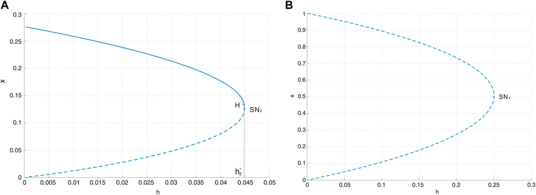
Figure 4. (A) Saddle-node bifurcation diagram SN₂ with a = 0.4, d = 0.6, and b = 0.5, where H represents the Hopf bifurcation point. The solid curve represents the stable equilibrium, and the dotted curve stands for the unstable equilibrium. (B) Saddle-node bifurcation diagram SN₁ with a = 0.4, d = 0.6, and b = 0.5.

Similar to the above discussion, we obtain

$S{N}_2=\left\{\left(a,b,d,h\right):h=h_2^{*},h_2^{*}<h_1^{*},a>0,b>0,d>0\right\},$

according to Theorem 3.2, is another saddle-node bifurcation surface. When the parameters transition from one side of the surface to the other, the number of positive equilibria in system Eq. 3 changes from zero to two. The saddle-node bifurcation is illustrated in Figure 4A.

4.2 Hopf bifurcation

From Theorem 3.6, we know that the positive equilibrium E₅ is a center-type nonhyperbolic equilibrium when b = b* and $h<\min \{h_1^{*},h_2^{*}\}$. Therefore, system (4) may undergo a Hopf bifurcation. To proceed, we first confirm the transversality condition necessary for a Hopf bifurcation,

$\frac{d}{db}Tr\left(J\left(E_5\right)\right){|}_{b=b^{*}}=-1\ne 0.$

Therefore, the stability of the positive equilibrium E₅ undergoes a change as the parameters traverse the specific critical surface

$H_1=\left\{\left(a,b,d,h\right):b=b^{*},h<\min \left\{h_1^{*},h_2^{*}\right\},a>0,d>0\right\}.$

To determine the direction of the Hopf bifurcation, we calculate the first Lyapunov number l₁ at the equilibrium E₅ = (x₅, y₅). Initially, we shift the equilibrium to the origin using the transformation $(\bar{x},\bar{y})=(x-x_5,y-y_5)$. Subsequently, we expand system Eq. 3 into a power series around the origin. Then, system Eq. 3 becomes

$\begin{array}{cc}\hfill \frac{d\bar{x}}{dt}& ={\alpha }_{10}\bar{x}+{\alpha }_{01}\bar{y}+{\alpha }_{20}{\bar{x}}^2+{\alpha }_{11}\bar{x}\bar{y}+{\alpha }_{30}{\bar{x}}^3+{\alpha }_{21}{\bar{x}}^2\bar{y}+P_{21}\left(\bar{x},\bar{y}\right),\hfill \\ \hfill \frac{d\bar{y}}{dt}& ={\beta }_{10}\bar{x}+{\beta }_{01}\bar{y}+{\beta }_{20}{\bar{x}}^2+{\beta }_{11}\bar{x}\bar{y}+{\beta }_{02}{\bar{y}}^2+{\beta }_{30}{\bar{x}}^3+{\beta }_{21}{\bar{x}}^2\bar{y}+{\beta }_{12}\bar{x}{\bar{y}}^2+Q_{21}\left(\bar{x},\bar{y}\right),\hfill \end{array}$

where $P_{21}(\bar{x},\bar{y})$ and $Q_{21}(\bar{x},\bar{y})$ are smooth functions of at least the fourth order with respect to $(\bar{x},\bar{y})$ and

$\begin{array}{cc}\hfill {\alpha }_{10}& =1-2x_5-\frac{\sqrt{x_5}}{2d{\left(1+a\sqrt{x_5}\right)}^2},{\alpha }_{01}=-\frac{\sqrt{x_5}}{1+a\sqrt{x_5}},{\alpha }_{11}=-\frac{1}{2\sqrt{x_5}{\left(1+a\sqrt{x_5}\right)}^2},\hfill \\ \hfill {\alpha }_{20}& =\frac{1+3a\sqrt{x_5}}{8d{x}_5{\left(1+a\sqrt{x_5}\right)}^3}-1,{\alpha }_{30}=-\frac{5a^2{x}_5+4a\sqrt{x_5}+1}{16d{x}_5^{\frac{3}{2}}{\left(1+a\sqrt{x_5}\right)}^4},{\alpha }_{21}=\frac{1+3a\sqrt{x_5}}{8x_5^{\frac{3}{2}}{\left(1+a\sqrt{x_5}\right)}^3},\hfill \\ \hfill {\beta }_{10}& =\frac{b}{d},{\beta }_{01}=-b,{\beta }_{20}=-\frac{b}{d{x}_5},{\beta }_{11}=\frac{2b}{x_5},{\beta }_{02}=-\frac{bd}{x_5},{\beta }_{30}=\frac{b}{d{x}_5^2},{\beta }_{21}=-\frac{2b}{x_5^2},\hfill \\ \hfill {\beta }_{12}& =\frac{bd}{x_5^2}.\hfill \end{array}$

In accordance with the formula for the first Lyapunov number l₁ presented in [24] [p.353], we proceed with the computation

$l_1=\frac{-3\pi }{2{\alpha }_{01}{\mathrm{\Delta }}^{\frac{3}{2}}}M,$

where

$\begin{array}{cc}\hfill M=& {\alpha }_{10}\left[{\alpha }_{11}{\beta }_{10}\left({\alpha }_{11}+{\beta }_{02}\right)+{\alpha }_{01}\left({\beta }_{11}^2+{\alpha }_{20}{\beta }_{11}+{\alpha }_{11}{\beta }_{02}\right)-2{\beta }_{10}{\beta }_{02}^2-2{\alpha }_{01}\left({\alpha }_{20}^2-{\beta }_{20}{\beta }_{02}\right)\right]\hfill \\ \hfill & -{\alpha }_{01}^2\left(2{\alpha }_{20}{\beta }_{20}+{\beta }_{11}{\beta }_{20}\right)+\left({\alpha }_{01}{\beta }_{10}-2{\alpha }_{10}^2\right)\left({\beta }_{11}{\beta }_{02}-{\alpha }_{11}{\alpha }_{20}\right)\hfill \\ \hfill & -\left({\alpha }_{10}^2+{\alpha }_{01}{\beta }_{10}\right)\left[-3{\alpha }_{01}{\alpha }_{30}+2{\alpha }_{10}\left({\alpha }_{21}+{\beta }_{12}-{\beta }_{21}{\beta }_{01}\right)\right],\hfill \end{array}$

and

$\mathrm{\Delta }={\alpha }_{10}{\beta }_{01}-{\alpha }_{01}{\beta }_{10}=Det\left[J\left(E_5\right)\right]>0,{\alpha }_{01}=-\frac{\sqrt{x_5}}{1+a\sqrt{x_5}}<0.$

Consequently, if l₁ < 0 (which corresponds to M < 0), then E₅ undergoes a supercritical Hopf bifurcation, leading to the emergence of a stable limit cycle in a small neighborhood of E₅ as the parameters across the surface H₁. Conversely, if l₁ > 0 (or M > 0), a subcritical Hopf bifurcation occurs, resulting in an unstable limit cycle appearing in the vicinity of E₅ as the parameters across the surface H₁.

Given the complexity of l₁, which does not readily reveal information about its sign, we turn to a numerical example for further clarification.

Fixing a = 0.4, d = 0.6, and h = 0.04, we obtain b* = 0.3960214438 and M = 0.537259605 and then l₁ > 0, which implies that an unstable limit cycle is created around E₅ = (0.1742665424, 00.2904442373). For b = 0.41 > b*, we obtain M = 0.652746120 and then l₁ > 0, which implies that an unstable limit cycle is created around E₅, where E₅ is asymptotically stable (see Figure 5B). When b = 0.425, a collision occurs between the periodic orbit and saddle E₄, resulting in the formation of a homoclinic orbit. Since M = 0.791862704, then l₁ > 0, which means that periodic orbits remain unstable, as shown in Figure 5A.

Figure 5

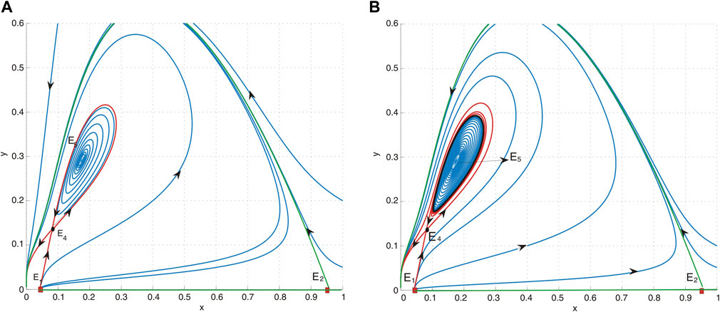
Figure 5. (A) Phase portrait of system (4) with a = 0.4, b = 0.425, d = 0.6, and h = 0.04. E₁ is an unstable node, E₂ is a saddle, E₄ is a saddle, and E₅ is a sink. It indicates that the periodic orbit undergoes a collision with the saddle E₄. (B) Phase portrait of system (4) with a = 0.4, b = 0.41, d = 0.6, and h = 0.04. E₁ is an unstable node, E₂ is a saddle, E₄ is a saddle, and E₅ is a sink. An unstable limit cycle, depicted as a black curve, surrounds the equilibrium point E₅.

4.3 Bogdanov–Takens bifurcation

As presented in Theorem 3.5, the positive equilibrium E₃ is identified as a cusp of co-dimension 2. This classification holds under certain conditions where a₁₀ + b₀₁ = 0, $h=h_2^{*}$, f₂₀ ≠ 0, and f₁₁ ≠ 0. Consequently, system Eq. 3 may undergo a Bogdanov–Takens bifurcation in the immediate vicinity of E₃.

Theorem 4.1. When h and d are selected as bifurcation parameters, system Eq. 3 is poised to experience a Bogdanov–Takens bifurcation in a neighborhood of E₃ as (h, d) varies near (h_BT, d_BT) for a₁₀ + b₀₁ = 0, $h=h_2^{*}$, f₂₀ ≠ 0, and f₁₁ ≠ 0, where (h_BT, d_BT) represents the threshold value of bifurcation parameters such as $Det(J(E_3)){\mid }_{(h,d)=(h_{BT},d_{BT})}=0$ and $Tr(J(E_3)){\mid }_{(h,d)=(h_{BT},d_{BT})}=0$.

Proof. To obtain the expressions for the saddle-node, Hopf, and homoclinic bifurcation curves, we derive a normal form for the Bogdanov–Takens bifurcation. This derivation uses the techniques outlined by [11, 18, 25].

Let us examine a perturbation of the parameters h and d centered around their BT bifurcation values. We represent this perturbation as h = h_BT + u and d = d_BT + v, where u and v are small deviations from the critical values h_BT and d_BT, respectively. Consider

$\begin{array}{cc}\hfill \frac{dx}{dt}& =x\left(1-x\right)-\frac{\sqrt{x}y}{1+a\sqrt{x}}-h_{BT}-u,\hfill \\ \hfill \frac{dy}{dt}& =by\left(1-\left(d_{BT}+v\right)\frac{y}{x}\right).\hfill & \hfill \end{array}(9)$

We begin by translating the equilibrium point E₃ = (x₃, y₃) to the origin using the transformations X = x − x₃ and Y = y − y₃. Subsequently, we expand system Eq. 9 as a power series centered at the origin. Then, we have

$\begin{array}{cc}\hfill \dot{X}& =m_{00}+m_{10}X+m_{01}Y+m_{11}XY+m_{20}{X}^2+P_1\left(X,Y\right),\hfill \\ \hfill \dot{Y}& =n_{00}+n_{10}X+n_{01}Y+n_{11}XY+n_{20}{X}^2+n_{02}{Y}^2+Q_1\left(X,Y\right),\hfill & \hfill \end{array}(10)$

where P₁(X, Y) and Q₁(X, Y) are smooth functions of at least the third order with respect to (X, Y), whose coefficients depend smoothly on u and v, and where

$\begin{array}{cc}\hfill m_{00}& =-u,m_{10}=1-2x_3-\frac{\sqrt{x_3}}{2d_{BT}{\left(1+a\sqrt{x_3}\right)}^2},m_{01}=-\frac{\sqrt{x_3}}{1+a\sqrt{x_3}},n_{00}=-\frac{bv{x}_3}{d_{BT}^2},\hfill \\ \hfill m_{11}& =-\frac{1}{2\sqrt{x_3}{\left(1+a\sqrt{x_3}\right)}^2},m_{20}=\frac{1+3a\sqrt{x_3}}{8d_{BT}{x}_3{\left(1+a\sqrt{x_3}\right)}^3}-1,n_{02}=-\frac{b\left(d_{BT}+v\right)}{x_3},\hfill \\ \hfill n_{10}& =\frac{b\left(d_{BT}+v\right)}{d_{BT}^2},n_{01}=-\frac{b\left(d_{BT}+2v\right)}{d_{BT}},n_{11}=\frac{2b\left(d_{BT}+v\right)}{x_3{d}_{BT}},n_{20}=-\frac{b\left(d_{BT}+v\right)}{x_3{d}_{BT}^2}.\hfill \end{array}$

Let x = X and y = m₀₀ + m₁₀X + m₀₁Y + m₁₁XY + m₂₀X² + P₁(X, Y), then system Eq. 10 can be written as

$\begin{array}{cc}\hfill \dot{x}& =y,\hfill \\ \hfill \dot{y}& =l_{00}+l_{10}x+l_{01}y+l_{11}xy+l_{20}{x}^2+l_{02}{y}^2+Q_2\left(x,y\right),\hfill \end{array}(11)$

where Q₂(x, y) are smooth functions of at least the third order with respect to (x, y), whose coefficients vary smoothly on u and v, and

$\begin{array}{cc}\hfill l_{00}=& \frac{m_{00}^2{n}_{02}-m_{00}{m}_{01}{n}_{01}+m_{01}^2{n}_{00}}{m_{01}},l_{01}=m_{10}+n_{01}-\frac{m_{00}\left(2n_{02}+m_{11}\right)}{m_{01}},\hfill \\ \hfill l_{10}=& m_{01}{n}_{10}-m_{00}{n}_{11}-m_{10}{n}_{01}+m_{11}{n}_{00}+\frac{m_{00}{n}_{02}\left(2m_{10}{m}_{01}-m_{00}{m}_{11}\right)}{m_{01}^2},\hfill \\ \hfill l_{20}=& m_{11}{n}_{10}-m_{10}{n}_{11}+m_{01}{n}_{20}+\frac{\left(2m_{00}{m}_{20}+m_{10}^2\right)n_{02}}{m_{01}}+\frac{m_{00}{m}_{11}{n}_{02}\left(m_{00}{m}_{11}-2m_{01}{m}_{10}\right)}{m_{01}^3},\hfill \\ \hfill l_{11}=& 2m_{20}+n_{11}+\frac{m_{00}{m}_{11}\left(m_{11}+2n_{02}\right)}{m_{01}^2}-\frac{m_{10}\left(m_{11}+2n_{02}\right)}{m_{01}},l_{02}=\frac{m_{11}+n_{02}}{m_{01}}.\hfill \end{array}$

By introducing a new variable τ through the relation dt = (1 − l₀₂x)dτ and subsequently rewriting τ back as t, we can recast system Eq. 11 in a new form:

$\begin{array}{cc}\hfill \dot{x}& =y\left(1-l_{02}x\right),\hfill \\ \hfill \dot{y}& =\left(1-l_{02}x\right)\left(l_{00}+l_{10}x+l_{01}y+l_{11}xy+l_{20}{x}^2+l_{02}{y}^2+Q_2\left(x,y\right)\right).\hfill \end{array}(12)$

Let X = x and Y = y(1 − l₀₂x), then system Eq. 12 can be written as

$\begin{array}{cc}\hfill \dot{X}& =Y,\hfill \\ \hfill \dot{Y}& =d_{00}+d_{10}X+d_{01}Y+d_{11}XY+d_{20}{X}^2+Q_3\left(X,Y\right),\hfill \end{array}(13)$

where Q₃(X, Y) are smooth functions of at least the third order with respect to (X, Y), whose coefficients depend smoothly on u and v, and

$\begin{array}{cc}\hfill d_{00}& =l_{00},d_{10}=l_{10}-2l_{00}{l}_{02},d_{01}=l_{01},d_{11}=l_{11}-l_{01}{l}_{02},\hfill \\ \hfill d_{20}& =l_{20}-2l_{10}{l}_{02}+l_{00}{l}_{02}^2.\hfill \end{array}$

Note that d₂₀ is very complex, and we cannot determine the sign of d₂₀ when u and v are small. Hence, we consider two cases: C-1: d₂₀ > 0; C-2: d₂₀ < 0.

C-1: If d₂₀ > 0 for small values of u and v, we perform the following change of variables: x = X, $y=\frac{Y}{\sqrt{d_{20}}}$, and $\tau =\sqrt{d_{20}}t$. Additionally, we retain variable t to represent τ. With these transformations, system Eq. 13 is transformed into a new form

$\begin{array}{cc}\hfill \dot{x}& =y,\hfill \\ \hfill \dot{y}& =h_{00}+h_{10}x+h_{01}y+h_{11}xy+x^2+Q_4\left(x,y\right),\hfill \end{array}(14)$

where Q₄(x, y) are smooth of at least the third order with respect to (x, y), whose coefficients depend smoothly on u and v, and

$h_{00}=\frac{d_{00}}{d_{20}},h_{10}=\frac{d_{10}}{d_{20}},h_{01}=\frac{d_{01}}{\sqrt{d_{20}}},h_{11}=\frac{d_{11}}{\sqrt{d_{20}}}.$

Let $X=x+\frac{h_{10}}{2}$ and Y = y, then system Eq. 14 can be written as

$\begin{array}{cc}\hfill \dot{X}& =Y,\hfill \\ \hfill \dot{Y}& =g_{00}+g_{01}Y+g_{11}XY+X^2+Q_5\left(X,Y\right),\hfill \end{array}(15)$

where Q₅(X, Y) are smooth of at least the third order with respect to (X, Y), whose coefficients depend smoothly on u and v, and

$g_{00}=h_{00}-\frac{1}{4}{h}_{10}^2,g_{01}=h_{01}-\frac{1}{2}{h}_{10}{h}_{11},g_{11}=h_{11}.$

Suppose d₁₁ ≠ 0, then g₁₁ = h₁₁ ≠ 0. Making the change of variables $x=g_{11}^{2}X$, $y=g_{11}^{3}Y$, and $\tau =\frac{1}{g_{11}}t$, we then obtain from system Eq. 15 that

$\begin{array}{cc}\hfill \dot{x}& =y,\hfill \\ \hfill \dot{y}& ={\mu }_1+{\mu }_{2}y+x^2+xy+Q_6\left(x,y\right),\hfill \end{array}$

where Q₆(x, y) are smooth of at least the third order with respect to (x, y), whose coefficients depend smoothly on u and v, and

${\mu }_1=g_{00}{g}_{11}^4,{\mu }_2=g_{01}{g}_{11}.(16)$

C-2: If d₂₀ < 0 for small u and v, we perform the following change of variables: x′ = X, $y^{\prime }=\frac{Y}{\sqrt{-d_{20}}}$, and ${\tau }^{\prime }=\sqrt{-d_{20}}t$. Additionally, we retain variable t to represent τ′. With these transformations, system Eq. 12 is transformed into a new form:

$\begin{array}{cc}\hfill \dot{x^{\prime }}& =y^{\prime },\hfill \\ \hfill \dot{y^{\prime }}& =h_{00}^{\prime }+h_{10}^{\prime }{x}^{\prime }+h_{01}^{\prime }{y}^{\prime }+h_{11}^{\prime }{x}^{\prime }{y}^{\prime }+x^{\prime 2}+Q_5^{\prime }\left(x^{\prime },y^{\prime },\epsilon \right),\hfill \end{array}(17)$

where $Q_5^{\prime }(x^{\prime },y^{\prime })$ are smooth of at least the third order with respect to (x′, y′), whose coefficients depend smoothly on u and v, and

$h_{00}^{\prime }=-\frac{d_{00}}{d_{20}},h_{10}^{\prime }=-\frac{d_{10}}{d_{20}},h_{01}^{\prime }=\frac{d_{01}}{\sqrt{-d_{20}}},h_{11}^{\prime }=\frac{d_{11}}{\sqrt{-d_{20}}}.$

Let $X^{\prime }=x^{\prime }-\frac{h_{10}^{\prime }}{2}$ and Y′ = y′, then system Eq. 17 can be written as

$\begin{array}{cc}\hfill \dot{X^{\prime }}& =Y^{\prime },\hfill \\ \hfill \dot{Y^{\prime }}& =g_{00}^{\prime }+g_{01}^{\prime }{Y}^{\prime }+g_{11}^{\prime }{X}^{\prime }{Y}^{\prime }+X^{\prime 2}+Q_6^{\prime }\left(X^{\prime },Y^{\prime }\right),\hfill \end{array}(18)$

where $Q_6^{\prime }(X^{\prime },Y^{\prime })$ are smooth of at least the third order with respect to (X′, Y′), whose coefficients depend smoothly on u and v, and

$g_{00}^{\prime }=h_{00}^{\prime }+\frac{1}{4}{h}_{10}^{\prime 2},g_{01}^{\prime }=h_{01}^{\prime }+\frac{1}{2}{h}_{10}^{\prime }{h}_{11}^{\prime },g_{11}^{\prime }=h_{11}^{\prime }.$

Suppose d₁₁ ≠ 0, $g_{11}^{\prime }=h_{11}^{\prime }\ne 0$. Making $x^{\prime }=-g_{11}^{\prime 2}{X}^{\prime }$, $y^{\prime }=g_{11}^{\prime 3}{Y}^{\prime }$, and ${\tau }^{\prime }=-\frac{1}{g_{11}}t$, we obtain the versal unfolding of system Eq. 18:

$\begin{array}{cc}\hfill \dot{x^{\prime }}& =y^{\prime },\hfill \\ \hfill \dot{y^{\prime }}& ={\mu }_1^{\prime }+{\mu }_2^{\prime }{y}^{\prime }+x^{\prime 2}+x^{\prime }{y}^{\prime }+Q_7^{\prime }\left(x^{\prime },y^{\prime }\right),\hfill \end{array}$

where $Q_7^{\prime }(x^{\prime },y^{\prime })$ are smooth of at least the third order with respect to (x′, y′), whose coefficients depend smoothly on u and v, and

${\mu }_1^{\prime }=-g_{00}^{\prime }{g}_{11}^{\prime 4},{\mu }_2^{\prime }=-g_{01}^{\prime }{g}_{11}^{\prime }.(19)$

To streamline the analysis, we retain the notation μ₁ and μ₂ for the transformed parameters ${\mu }_1^{\prime }$ and ${\mu }_2^{\prime }$, as defined in Equation Eq. 19. This approach reduces the number of cases we must consider. If the Jacobian determinant $|\frac{\partial ({\mu }_1,{\mu }_2)}{\partial (u,v)}{|}_{(u,v)=(\mathrm{0,0})}$ is non-zero, then the parameter transformations described by Eqs 16 and 19 are homeomorphisms in a small neighborhood of the origin. Consequently, μ₁ and μ₂ can be treated as independent parameters.

Drawing upon the findings obtained by [24] and as supported by [5, 11, 18, 26], we establish that system Eq. 9 experiences a Bogdanov–Takens bifurcation when the parameters (u, v) are in a small neighborhood of the origin. The local representatisons of the bifurcation curves, derived from the analysis, are as follows (“+” for d₂₀ > 0, “-” for d₂₀ < 0):

(1) The saddle-node bifurcation curve SN = {(u, v): μ₁ = 0, μ₂ ≠ 0};

(2) The Hopf bifurcation curve $H=\{(u,v):{\mu }_2=\pm \sqrt{-{\mu }_1},{\mu }_1<0\}$;

(3) The homoclinic bifurcation curve $HL=\{(u,v):{\mu }_2=\pm \frac{5}{7}\sqrt{-{\mu }_1},{\mu }_1<0\}$.

Subsequently, we numerically illustrate the locations of the bifurcation curves and the dynamics of the system at the Bogdanov–Takens bifurcation point. This is achieved by selecting specific values for the dimensionless parameters. We choose a = 0.4 and d_BT = 0.6, then h_BT = 0.04485055333 and b = 0.5193087015. Since d₂₀ = 1729.213892u² − 1.159964346–9.646351129v − 31.60626034u − 319.1508390uv and d₁₁ = (22.77081918–346.0816837u)v² + (19.64233118–642.5091021u)v − 284.7831954u − 2.673388394, then d₂₀ < 0 and d₁₁ ≠ 0 for u ∈ (−0.01, 0.01) and v ∈ (−0.1, 0.1), so we compute Eq. 19 and get $|\frac{\partial ({\mu }_1,{\mu }_2)}{\partial (u,v)}{|}_{(u,v)=(\mathrm{0,0})}=-14.3295339671392\ne 0$. Hence, the parameter transformation Eq. 19 is nonsingular. The local representations of the bifurcation curves up to second-order approximations are as follows:

(1) The saddle-node bifurcation curve $\begin{array}{l}SN=\left\{(u,v):{\mu }_2\ne 0,-1.86375448162305v\right.+16.9957334575794u\\ +4614.59435174402u^2-1401.21892975004uv+98.3266830247282v^2\};\end{array}$

(2) The Hopf bifurcation curve $\begin{array}{l}H=\left\{(u,v):{\mu }_1<0,-1.86375448162305v\right.+16.9957334575794u+\\ 4784.69223204402u^2-1460.51719203213uv+103.494713194792v^2\};\end{array}$

(3) The homoclinic bifurcation curve $\begin{array}{l}HL=\left\{(u,v):{\mu }_1<0,-0.950895143738617v\right.+8.67129258088447u+\\ 2524.48275351690u^2-774.205879496251uv+55.3347051835753v^2\}.\end{array}$

These bifurcation curves H, HL, and SN divide the small neighborhood of the origin in the parameter plane (u, v) into four regions. The bifurcation diagram of system Eq. 9 is given in Figure 6A, from which we obtain the following observations:

Figure 6

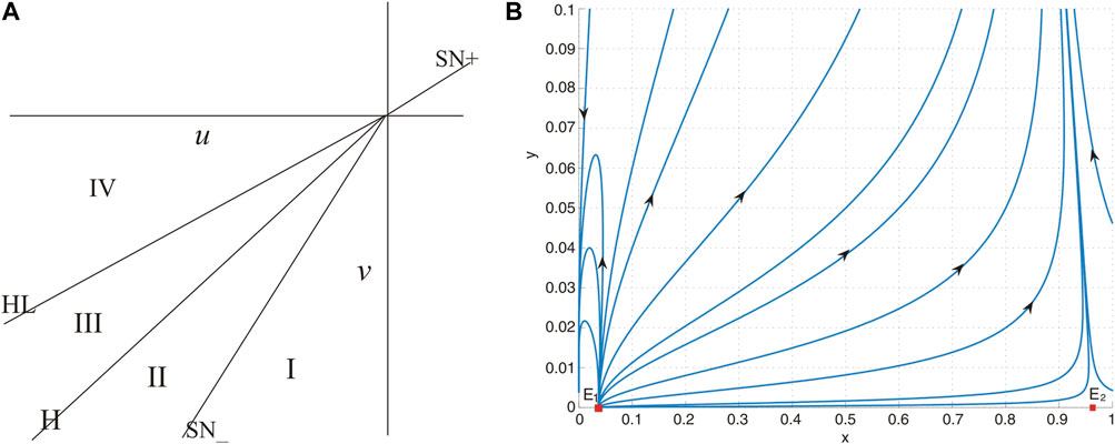
Figure 6. (A) Bifurcation diagram of system (26). (B) No positive equilibrium when (u, v) = (−0.01, − 0.1) lies in region I, and system (26) has two boundary equilibria E₁ and E₂.

(a) When (u, v) = (0, 0), the unique positive equilibrium is a cusp of co-dimension 2.

(b) When the parameters are situated within region I, the system lacks a positive equilibrium, as shown in Figure 6B. This absence implies that the prey population is inclined toward extinction under nearly all initial conditions.

(c) When the parameters are positioned along the curve SN, the system exhibits a positive equilibrium that is characterized as a saddle node.

(d) In region II, system Eq. 9 possesses two positive equilibria. Specifically, E₄ is identified as a saddle, while E₅ acts as a source, as shown in Figure 7A.

(e) Upon crossing curve H and entering region III, the system undergoes a subcritical Hopf bifurcation, resulting in the emergence of an unstable limit cycle. This phenomenon is depicted in Figure 7B.

(f) When the parameters are selected along the curve HL, an unstable homoclinic cycle encircles a sink, while the other equilibrium remains a saddle. This configuration is illustrated in Figure 8A.

(g) In region IV, the system is characterized by the presence of a sink and a saddle, as depicted in Figure 8B.

Figure 7

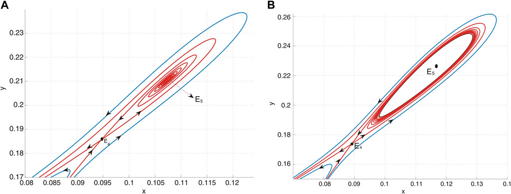
Figure 7. (A) E₅ is a source and E₄ is a saddle when (u, v) = (−0.01, − 0.09) lies in region II. (B) E₅ is a sink and E₄ is a saddle when (u, v) = (−0.01, − 0.087) lies in region III, and an unstable limit cycle encloses E₅.

Figure 8

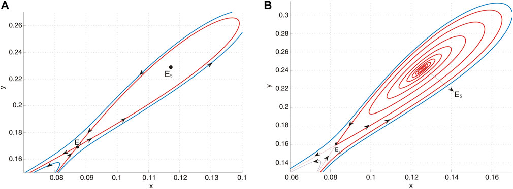
Figure 8. (A) E₅ is a sink and E₄ is a saddle when (u, v) = (−0.01, − 0.0854) lies on curve HL and an unstable homoclinic orbit encloses E₅. (B) E₅ is a sink and E₄ is a saddle when (u, v) = (−0.01, − 0.08) lies in region IV.

5 Conclusion

In this paper, we explore a Leslie-type predator–prey system incorporating prey harvesting. Initially, we examine system Eq. 2 without prey harvesting, establishing that it possesses a unique boundary equilibrium and a unique positive equilibrium. Theorem 2.2 elucidates the stability of both boundary equilibrium and positive equilibrium. Notably, the boundary equilibrium is consistently unstable, indicating that neither the prey nor the predator will ever become extinct without the influence of prey harvesting.

Furthermore, we study the dynamic behaviors of system Eq. 3 to analyze the effect of prey harvesting on the prey and predator. Hence, we first analyze the existence and stability of equilibria for system Eq. 3 in Section 3. As shown in Theorem 3.1, we identify the maximum sustainable yield as $h_{\mathit{MSY}}=\frac{1}{4}$. Beyond this threshold $(h>\frac{1}{4})$, both the prey and predator species face extinction. Our investigation into the stability of the positive equilibria reveals that the coexistence of both species is possible if $b>b_1^{*}$ and the harvesting rate $h=h_2^{*}$ is between $h_1^{*}$ and h_MSY, or if b⩾b* and h is less than the minimum of $h_1^{*}$ and $h_2^{*}$. Otherwise, either only the prey survives or both species become extinct. This insight underscores the importance of selecting an appropriate harvesting rate, specifically one that is below a critical threshold and less than h_MSY to ensure the coexistence of the predator and prey, thereby sustaining ecological balance.

In Section 4, we chose the constant harvesting rate h as one of the bifurcation parameters to perform the bifurcation analysis of system Eq. 3. We find that system Eq. 3 has complex dynamic behavior and undergoes Hopf bifurcation, Bogdanov–Takens bifurcation of co-dimension 2, and saddle-node bifurcation. Among them, the emergence of saddle-node bifurcation means that system Eq. 3 has bi-stable behavior, and the prey may face extinction or sustain, which depends on the harvesting rate. For the Hopf bifurcation, we calculate the first Lyapunov number to ascertain the direction of the Hopf bifurcation, which indicates whether a stable or unstable limit cycle emerges in the vicinity of the equilibrium E₅. By selecting two parameters from system Eq. 3 as bifurcation parameters, we demonstrate that the system undergoes a Bogdanov–Takens bifurcation of co-dimension 2. This conclusion is drawn from our analysis of the universal unfolding near the cusp.

In conclusion, we constructed and provided a detailed dynamic analysis of a Leslie-type predator–prey system that incorporates prey harvesting. Our findings reveal that prey harvesting introduces complex dynamic behaviors into the system, potentially leading to a series of bifurcations. Furthermore, if the harvesting intensity exceeds a critical threshold, the prey may face extinction. These insights offer valuable contributions to the understanding of predator–prey systems and ecological balance. However, it is worth noting that this paper focuses primarily on qualitative analysis and lacks empirical data to support our theoretical findings. Despite this, significant algorithms have been developed to gather and analyze real-world data. We intend to leverage these algorithms to quantitatively assess the impact of harvesting using the methodologies introduced by [27, 28]. Additionally, this study does not consider the removal of both prey and predator species, and human activity can significantly impact ecosystems, as highlighted by [29]. Drawing inspiration from [30–36], our model can be extended to eco-epidemic systems and reaction–diffusion systems. These areas represent promising directions for future research in this field.

Data availability statement

The original contributions presented in the study are included in the article/Supplementary Material; further inquiries can be directed to the corresponding author.

Author contributions

YZ: data curation, methodology, writing–original draft, and writing–review and editing. JL: methodology, writing–original draft, and writing–review and editing.

Funding

The author(s) declare that financial support was received for the research, authorship, and/or publication of this article. The research was supported by the National Natural Science Foundation of China (No. 12201582), Research Project Supported by Shanxi Scholarship Council of China (2022-151), and the Fundamental Research Program of Shanxi Province under grant (No. 202203021212130).

Conflict of interest

The authors declare that the research was conducted in the absence of any commercial or financial relationships that could be construed as a potential conflict of interest.

Publisher’s note

All claims expressed in this article are solely those of the authors and do not necessarily represent those of their affiliated organizations, or those of the publisher, the editors, and the reviewers. Any product that may be evaluated in this article, or claim that may be made by its manufacturer, is not guaranteed or endorsed by the publisher.

References

1. Ning L-Y, Luo X-F, Li B-L, Wu Y-P, Sun G-Q, Feng T-C An effective allee effect may induce the survival of low-density predator. Results Phys (2023) 53:106926.

CrossRef Full Text | Google Scholar

2. May R Stability and complexity in model ecosystems. Princeton: Princeton University Press (1973).

Google Scholar

3. Seo G, DeAngelis DL A predator-prey model with a holling type i functional response including a predator mutual interference. J Nonlinear Sci (2011) 21:811–33. doi:10.1007/s00332-011-9101-6

CrossRef Full Text | Google Scholar

4. Hsu S, Huang T Global stability for a class of predator-prey system. SIAM J Appl Math (1995) 6:763–83.

CrossRef Full Text | Google Scholar

5. Huang J, Ruan S, Song J Bifurcations in a predator-prey system of leslie type with generalized holling type iii functional response. J Differ Equations (2014) 257:1721–52. doi:10.1016/j.jde.2014.04.024

CrossRef Full Text | Google Scholar

6. Liu C, Chang L, Huang Y, Wang Z Turing patterns in a predator-prey model on complex networks. Nonlinear Dyn (2020) 99:3313–22. doi:10.1007/s11071-019-05460-1

CrossRef Full Text | Google Scholar

7. Huang J, Xiao D Analyses of bifurcations and stability in a predator-prey system with holling type-iv functional response. Acta Math Appl Sin Engl Ser (2004) 20:167–78.

Google Scholar

8. Li Y, Xiao D Bifurcations of a predator-prey system of holling and lesile types. Chaos Soliton Fract (2007) 34:606–20.

CrossRef Full Text | Google Scholar

9. Bera S, Maiti A, Samanta G Stochastic analysis of a prey-predator model with herd behaviour of prey. Nonlinear Anal.-Model. (2016) 21:345–61. doi:10.15388/na.2016.3.4

CrossRef Full Text | Google Scholar

10. Braza A Predator-prey dynamics with square root functional responses. Nonlinear Anal.-Real (2012) 13:1837–43. doi:10.1016/j.nonrwa.2011.12.014

CrossRef Full Text | Google Scholar

11. Hu D, Cao H Stability and bifurcation analysis in a predator–prey system with Michaelis–Menten type predator harvesting. Nonlinear Anal.-Real (2017) 33:58–82. doi:10.1016/j.nonrwa.2016.05.010

CrossRef Full Text | Google Scholar

12. Gupta R, Chandra P Bifurcation analysis of modified leslie-gower predator-prey model with michaelis-menten type prey harvesting. J Math Anal Appl (2003) 398:278–95. doi:10.1016/j.jmaa.2012.08.057

CrossRef Full Text | Google Scholar

13. Das T, Mukherjee R, Chaudhari K Bioeconomic harvesting of a prey-predator fishery. J Biol Dyn (2009) 3:447–62. doi:10.1080/17513750802560346

PubMed Abstract | CrossRef Full Text | Google Scholar

14. Chakraborty K, Jana S, Kar T Global dynamics and bifurcation in a stage structured prey-predator fishery model with harvesting. Appl Math Comput (2012) 218:9271–90. doi:10.1016/j.amc.2012.03.005

CrossRef Full Text | Google Scholar

15. Rojas-Palma A, Gonz’alez-Olivares E Optimal harvesting in a predator-prey model with allee effect and sigmoid functional response. Appl Math Model (2012) 36:1864–74. doi:10.1016/j.apm.2011.07.081

CrossRef Full Text | Google Scholar

16. Xiao D, Ruan S Bogdanov-takens bifurcations in predator-prey systems with constant rate harvesting. Fields Inst Commun (1999) 21:493–506. doi:10.1090/fic/021/41

CrossRef Full Text | Google Scholar

17. Peng G, Jiang Y, Li C Bifurcations of a holling-type ii predator-prey system with constant rate harvesting. Int J Bifurcat Chaos (2009) 19:2499–514. doi:10.1142/s021812740902427x

CrossRef Full Text | Google Scholar

18. Huang J, Gong Y, Chen J Multiple bifurcations in a predator-prey system of holling and leslie type with constant-yield prey harvesting. Int J Bifurcat Chaos (2013) 23:1350164. doi:10.1142/s0218127413501642

CrossRef Full Text | Google Scholar

19. Zhu C, Lan K Phase portraits, hopf-bifurcations and limit cycles of leslie-gower predator-prey systems with harvesting rates. Discrete Contin Dyn Syst Ser B (2010) 14:289–306. doi:10.3934/dcdsb.2010.14.289

CrossRef Full Text | Google Scholar

20. Xiao D, Jennings LS Bifurcations of a ratio-dependent predator-prey system with constant rate harvesting. SIAM J Appl Math (2005) 65:737–53. doi:10.1137/s0036139903428719

CrossRef Full Text | Google Scholar

21. Xiao D, Li W, Han M Dynamics in a ratio-dependent predator-prey model with predator harvesting. J Math Anal Appl (2006) 324:14–29. doi:10.1016/j.jmaa.2005.11.048

CrossRef Full Text | Google Scholar

22. Luo J, Zhao Y Stability and bifurcation analysis in a predator-prey system with constant harvesting and prey group defense. Int J Bifurcat Chaos (2017) 27:1750179. doi:10.1142/s0218127417501796

CrossRef Full Text | Google Scholar

23. Zhang Z, Ding T, Huang W, Dong Z Qualitative theory of differential equation. Beijing: Science Press (1992).

Google Scholar

24. Perko L Differential equations and dynamical systems. 3rd ed. New York: Springer-Verlag (2000).

Google Scholar

25. Chen J, Huang J, Ruan S, Wang J Bifurcations of invariant tori in predator-prey models with seasonal prey harvesting. SIAM J Appl Math (2013) 73:1876–905. doi:10.1137/120895858

CrossRef Full Text | Google Scholar

26. Huang J, Gong Y, Ruan S Bifurcation analysis in a predator-prey model with constant-yield predator harvesting. Discrete Contin Dynam Syst Ser B (2013) 18:2101–21. doi:10.3934/dcdsb.2013.18.2101

CrossRef Full Text | Google Scholar

27. Li H, Cao H, Feng Y, Li X, Pei J Optimization of graph clustering inspired by dynamic belief systems. IEEE Trans Knowledge Data Eng (2023) 1–14. doi:10.1109/TKDE.2023.3274547

CrossRef Full Text | Google Scholar

28. Li H, Feng Y, Xia C, Cao J Overlapping graph clustering in attributed networks via generalized cluster potential game. ACM T Knowl Discov D (2023) 18:1–26. doi:10.1145/3597436

CrossRef Full Text | Google Scholar

29. Hou L-F, Sun G-Q, Perc M The impact of heterogeneous human activity on vegetation patterns in arid environments. Communical Nonlinear SCI (2023) 126:107461. doi:10.1016/j.cnsns.2023.107461

CrossRef Full Text | Google Scholar

30. Fu S, Luo J, Zhao Y Stability and bifurcations analysis in an ecoepidemic system with prey group defense and two infectious routes. Math Comput Simulat (2023) 205:581–99.

Google Scholar

31. Gao S, Chang L, Perc M, Wang Z Turing patterns in simplicial complexes. Phys Rev E (2023) 107:014216. doi:10.1103/physreve.107.014216

CrossRef Full Text | Google Scholar

32. Wang C, Chang L, Liu H Spatial patterns of a predator-prey system of leslie type with time delay. PLoS One (2016) 11:e0150503. doi:10.1371/journal.pone.0150503

CrossRef Full Text | Google Scholar

33. Liang J, Sun G-Q Effect of nonlocal delay with strong kernel on vegetation pattern. J Appl Anal Comput (2024) 14:473–505. doi:10.11948/20230290

CrossRef Full Text | Google Scholar

34. Yang J, Gong M, Sun G-Q Asymptotical profiles of an age-structured foot-and-mouth disease with nonlocal diffusion on a spatially heterogeneous environment. J Differ Equations (2023) 377:71–112. doi:10.1016/j.jde.2023.09.001

CrossRef Full Text | Google Scholar

35. Liu S-M, Bai Z, Sun G-Q Global dynamics of a reaction-diffusion brucellosis model with spatiotemporal heterogeneity and nonlocal delay. Nonlinearity (2023) 36:5699–730. doi:10.1088/1361-6544/acf6a5

CrossRef Full Text | Google Scholar

36. He R, Luo X, Asamoah JKK, Zhang Y, Li Y, Jin Z, et al. A hierarchical intervention scheme based on epidemic severity in a community network. J Math Biol (2023) 87:29. doi:10.1007/s00285-023-01964-y

CrossRef Full Text | Google Scholar