Maximizing the symmetry of Maxwell’s equations

Maxwell’s equations can be successfully extended to electromagnetic fields having three complex-valued components rather than their usual three real-valued components. Here the implications of interpreting the imaginary-valued components as extending into time rather than space are explored. The complex-valued Maxwell equations remain consistent with the original Maxwell equations and the experimental results that they predict. Further, the extended equations predict novel phenomena such as the existence of electromagnetic waves that propagate not only through regular space but also through a separate temporal space (time) that is implied by the three imaginary components of the fields. In a vacuum, part of these imaginary valued waves propagates through time at the same rate as an observer stationary in space. While the imaginary valued field components are not directly observable, analysis indicates that they should be indirectly detectable experimentally based on secondary effects that occur under special circumstances. Experimental investigation attempting to falsify or support the existence of complex valued electromagnetic fields extending into time is merited due to the substantial theoretical and practical implications involved.

1 Introduction

Maxwell’s Equations, the foundation of classical electrodynamics, exhibit a number of widely recognized asymmetries [1–3]. However, it has recently been shown that these asymmetries can be lessened while still retaining consistency with known experimental results by assuming that electromagnetic fields have three complex-valued components rather than three real-valued components [4], as in

$\mathit{E}=\left[\begin{array}{c}{E}_{x1}+i{E}_{t1}\\ E_{x2}+i{E}_{t2}\\ E_{x3}+i{E}_{t3}\end{array}\right]={\mathit{E}}_{\mathit{x}}+i{\mathit{E}}_t(1.1)$

where $i=\sqrt{-1}$, and ${\mathit{E}}_x=\left[\begin{array}{c}{E}_{x1}\\ E_{x2}\\ E_{x3}\end{array}\right]$ and i ${\mathit{E}}_t=i\left[\begin{array}{c}{E}_{t1}\\ E_{t2}\\ E_{t3}\end{array}\right]$ are, respectively, the usual real-valued electric field vector in the classic Maxwell equations, and new imaginary-valued quantities that are assumed to exist in a transcendent part of space and to be unobservable. When Maxwell’s equations are modified to accommodate such complex-valued fields, the resulting formulation remains consistent with the original Maxwell equations, and with existing experimental findings such as conservation of charge and observable energy. The extended equations exhibit increased symmetry in the form of an electromagnetic duality transformation, and they predict the existence of magnetic monopoles while also providing a novel explanation for why these monopoles have escaped detection during past experimental searches.

This development of the complex-valued version of Maxwell’s equations, solely within the scope of classical electromagnetism, was largely guided by efforts to increase the symmetry of these equations while retaining their simplicity and consistency with known experimental results. The resulting complex-valued equations increase the symmetry of the original Maxwell equations in two ways (items one and two of Table 1). First, classical theory posits that only electric charge exists, while the complex-valued theory generalizes this by predicting that both electric and magnetic charge exist. Second, previous discussions about the existence of magnetic charge have largely assumed that magnetic monopoles are separate entities from electric charge, while in contrast the complex-valued equations take magnetic and electric charge to be one and the same physical entity.

Table 1

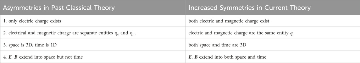
Table 1. Maximizing the symmetry of Maxwell’s equations.

The novelty of these first two modifications can be clarified by considering how the idea of hypothetical magnetic charge is typically illustrated within classical electrodynamics by modifying Maxwell’s equations to be

$\nabla \cdot \mathit{E}=\frac{1}{{ϵ}_0}\rho (\mathrm{1.2a})$

$\nabla \hspace{0.17em}\times \mathit{E}=-{\mu }_0{\mathit{J}}_m-\frac{\partial \mathit{B}}{\partial t}(\mathrm{1.2b})$

$\nabla \cdot \mathit{B}={\mu }_0{\rho }_m(\mathrm{1.2c})$

$\nabla \hspace{0.17em}\times \mathit{B}={\mu }_0\mathit{J}+\frac{1}{c^2}\frac{\partial \mathit{E}}{\partial t}(\mathrm{1.2d})$

[2,3,5,6], where there are two significant additions to the classic Maxwell’s equations. Here E (B) is the 3-component electric (magnetic) field, c is the speed of light, ${ϵ}_0$ (${\mu }_0$) is the permittivity (permeability) of free space, ρ is the electric charge density, and J is the volume electric current density. Eqs. 1.2 are an extension of Maxwell’s equations where the normal zero on the right hand side of Eq. 1.2c has been replaced with a “missing” magnetic charge density ${\rho }_m$ term, making it more symmetric with Eq. 1.2a, and a new magnetic current density term ${\mathit{J}}_m$ has been added on the right side of Eq. 1.2b to make it more symmetric with Eq. 1.2d. While these extended Maxwell’s equations exhibit a beautiful symmetry that is formally represented by an electromagnetic duality transformation, this symmetry is marred by the fact that extensive experimental search efforts (using modern accelerators, examining cosmic rays, etc.) have repeatedly failed to find the magnetic monopoles implied by these extensions, suggesting to many that such monopoles are rare and/or extremely massive, or that they simply do not exist so that the extended Eqs. 1.2 are inconsistent with experiment.

In contrast, if one introduces complex-valued electromagnetic fields where the imaginary portions are taken to be unobservable, one can replace density ${\rho }_m$ with $i\rho$ and ${\mathit{J}}_m$ with $i\mathit{J}$ in Eqs. 1.2, retaining the increased symmetry associated with theorized magnetic monopoles, and explaining why these monopoles have not been found experimentally: their magnetic fields are purely imaginary-valued and not observable. Further, this is achieved without introducing a new type of magnetic charge: a single charged particle such as an electron or proton serves as a source/sink for both real-valued and imaginary-valued fields. This latter concept differs from that of a dyon which similarly has both electric and magnetic fields [7], but unlike what is considered here both of the dyon’s fields have only real-valued components (dyons have also not been found in experimental searches so far [8]).

While the earlier complex-valued Maxwell equations are more symmetric and consistent with previous negative experimental searches for magnetic monopoles, they are also limited in that they continue to exhibit other asymmetries. It thus seems reasonable to inquire whether there are additional ways to increase the symmetry of these equations without leading to contradictions with known experimental findings. If so, it is of interest to explore what the implications of such an extension would be, and whether their novel predictions might be verified or falsified. Specifically, another asymmetry of Maxwell’s equations, and one that was retained in the previously derived complex-valued version of these equations [4], is the assumption of an underlying 4D spacetime reminiscent of Minkowski spacetime, having one real-valued temporal dimension but three complex-valued spatial dimensions.

To address this issue, here we investigate the implications of increasing the symmetry of space and time in Maxwell’s equations, expressing this as the temporal fields hypothesis:Electromagnetic fields have imaginary-valued components that extend into time.

This hypothesis is examined by interpreting the unobservable imaginary components of electromagnetic fields as extending into time, rather than into space as was done previously in [4]. Since each electromagnetic field vector, like in Eq. 1.1, has three imaginary components, this indicates that time, like space, must in some sense be considered to be three dimensional (item three in Table 1), placing space and time on a more symmetrical footing in that each now has three dimensions. The specific motivation for proposing multi-dimensional time is that the fields represented by the complex-valued Maxwell equations have three imaginary components, so taking them to exist in a 3D temporal space leads to increased symmetry and simplicity of these equations. In particular, this leads to the temporal fields hypothesis above that electromagnetic fields have components extending into time as well as space (item 4, Table 1).

In the following, solely within the framework of classical electromagnetism (no consideration of gravity or quantum physics), the complex-valued Maxwell equations are described, some of their basic properties are discussed, and two types of duality transforms are given (Section 2). A Lorentz transformation generalized to a three dimensional complex space ${\mathbb{C}}^3$ is described, a spacetime interval generalized to ${\mathbb{C}}^3$ is shown to be invariant under this transformation, and this interval is found to imply a universal speed constraint on all physical entities (Section 3). A wave equation is then derived in the usual way but now from the complex valued Maxwell equations, resulting in the prediction that the imaginary components of electromagnetic waves move through time, and surprisingly do so at the same speed in a vacuum as an observer at rest in space does (Section 4). While the imaginary components of complex electromagnetic fields are unobservable directly, falsifying or supporting the temporal fields hypothesis experimentally should be possible by detecting indirect effects that the imaginary components produce under special but realizable conditions (Section 5). A brief assessment and discussion of limitations is given (Section 6).

2 Complex-valued electromagnetic fields

In this section, a version of Maxwell’s equations accommodating complex-valued electromagnetic fields extending into time is described, and two duality transformations are given to indicate more formally the resulting increased symmetry.

2.1 Accommodating complex fields with temporal imaginary-valued components

The complex-valued Maxwell equations considered here are given by:

$\nabla \cdot \mathit{E}=\frac{1}{{ϵ}_0}\rho (\mathrm{2.1a})$

$\nabla \hspace{0.17em}\times \mathit{E}={-ic\mu }_0\mathit{J}-\frac{\partial \mathit{B}}{\partial t}(\mathrm{2.1b})$

$\nabla \cdot \mathit{B}={ic\mu }_0\rho (\mathrm{2.1c})$

$\nabla \hspace{0.17em}\times \mathit{B}={\mu }_0\mathit{J}+\frac{1}{c^2}\frac{\partial \mathit{E}}{\partial t}(\mathrm{2.1d})$

These equations indicate that both electric and magnetic charge exist, and that they are the same entity (items 1, 2 in Table 1). Here E (B) is the complex electric (magnetic) field in ${\mathbb{C}}^3$, bold font indicates 3-component column vectors, and SI units are assumed. While these equations superficially appear to be similar to Maxwell’s original equations extended as in Eqs. 1.2, they differ in very substantial ways. The electric and magnetic field vectors E and B that appear here have complex-valued components,

$\begin{array}{cc}\mathit{E}=\left[\begin{array}{c}{E}_{x1}+i{E}_{t1}\\ E_{x2}+i{E}_{t2}\\ E_{x3}+i{E}_{t3}\end{array}\right]={\mathit{E}}_{\mathit{x}}+i{\mathit{E}}_t& \mathit{B}=\left[\begin{array}{c}{B}_{x1}+i{B}_{t1}\\ B_{x2}+i{B}_{t2}\\ B_{x3}+i{B}_{t3}\end{array}\right]={\mathit{B}}_{\mathit{x}}+i{\mathit{B}}_t\end{array}(2.2)$

where

$\begin{array}{cccc}{\mathit{E}}_x=\left[\begin{array}{c}{E}_{x1}\\ E_{x2}\\ E_{x3}\end{array}\right]& {\mathit{E}}_t=\left[\begin{array}{c}{E}_{t1}\\ E_{t2}\\ E_{t3}\end{array}\right]& {\mathit{B}}_x=\left[\begin{array}{c}{B}_{x1}\\ B_{x2}\\ B_{x3}\end{array}\right]& {\mathit{B}}_t=\left[\begin{array}{c}{B}_{t1}\\ B_{t2}\\ B_{t3}\end{array}\right]\end{array}(2.3)$

are vectors in 3D real-valued space ${\mathbb{R}}^3$. These fields are assumed to be functions of location in a spacetime whose points are represented by $\mathit{s}=\mathit{x}+ic\mathit{t}$, where x and t are both 3D real-valued vectors and the latter is associated with time. However, the real valued variable t that appears in $\partial t$ in Eqs. 2.1 remains the familiar clock time–its relation to the vector t is described in Section 3. Vectors E_x and B_x are the usual electric and magnetic fields as they currently appear in Maxwell’s original equations. In contrast, E_t and B_t in Eq. 2.2, both lying in ${\mathbb{R}}^3$, indicate that electromagnetic fields have imaginary-valued portions i E_t and i B_t of their components that are unobservable and that are interpreted as extending into time.

It is helpful to introduce some terminology and concepts that facilitate visualization of these fields. Their real field portions E_x and B_x are said to lie in real-valued space, or r-space, that corresponds to familiar and observable 3D space used by the classical Maxwell equations. In contrast, E_t and B_t are taken to exist in a separate temporal space or t-space that is tightly linked to the notion of clock time t. To facilitate visualizing these fields, it helps to think of the complex-valued fields E and B in two different but equivalent ways. First, we can view each of their three field components as lying in the complex (Argand) plane, as shown on the left in Figure 1. Alternatively, we can think of the real and imaginary portions of fields E and B as lying in two 3D spaces, as illustrated on the right in Figure 1. The latter viewpoint is adopted here–it makes the observable vs. unobservable distinction between real-valued spatial and imaginary-valued temporal components explicit. The classical Maxwell equations based on E_x and B_x assume the familiar 3D r-space that is observable, while the imaginary portions E_t and B_t of the complex fields E and B lie in unobservable t-space, which is called “temporal” to emphasize its relationship to familiar clock time t. The formulation of electromagnetism considered here only hypothesizes that electromagnetic fields extend into t-space; it does not assume a priori that matter, charge or any other physical entities extend into t-space.

Figure 1

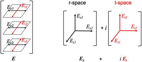
Figure 1. Two different geometric conceptions of the complex-valued field E (analogous comments apply to B). On the left, each component of E lies in a complex-valued plane. On the right, E is viewed as the sum of 3D real-valued E_x in r-space and 3D imaginary-valued i E_t in t-space. Vector E_t itself is real-valued. Red indicates imaginary-valued axes and components.

As with Eqs. 1.2b, 1.2c which include hypothetical magnetic monopoles, Eqs. 2.1b, 2.1c include new terms on their right sides that imply the existence of magnetic charge and current, increasing the underlying symmetry. However, unlike Eqs. 1.2, these terms are purely imaginary, thus explicitly implying the existence of imaginary components in the fields E and B. Further, these terms differ in using $\rho$ and $\mathit{J}$ rather than ${\rho }_m$ and ${\mathit{J}}_m$ as in Eqs. 1.2, and therefore they do not imply the existence of a novel kind of magnetically charged particle.

Eqs. 2.1 also differ from the classic Maxwell’s equations in that the divergence $\nabla \cdot$ and curl $\nabla \times$ operations generalized to complex fields are not the typical operators that one might expect. These non-standard reduction vector operators provide convenient abbreviations whereby vector product operations in a 3D complex space ${\mathbb{C}}^3$ are “reduced” to a linear sum of the standard corresponding ${\mathbb{R}}^3$ operations in r-space and t-space. If $\mathit{C}={\mathit{C}}_{\mathit{x}}+i{\mathit{C}}_{\mathit{t}}$ and ${\mathit{C}}^{\prime }={\mathit{C}}_{\mathit{x}}^{\prime }+i{\mathit{C}}_t^{\prime }$ are two arbitrary vectors in ${\mathbb{C}}^3$ where ${\mathit{C}}_{\mathit{x}},{\mathit{C}}_{\mathit{t}}$, ${\mathit{C}}_{\mathit{x}}^{\prime }$ and ${\mathit{C}}_t^{\prime }$ all lie in ${\mathbb{R}}^3$, the reduction dot product $\cdot$ and cross product $\times$ of $\mathit{C}$ and ${\mathit{C}}^{\prime }$ in ${\mathbb{C}}^3$ are defined to be

$\mathit{C}\cdot {\mathit{C}}^{\prime }={\mathit{C}}_{\mathit{x}}\cdot {\mathit{C}}_{\mathit{x}}^{\prime }+i{\mathit{C}}_{\mathit{t}}\cdot {\mathit{C}}_{\mathit{t}}^{\prime }(\mathrm{2.4a})$

$\mathit{C}\times {\mathit{C}}^{\prime }={\mathit{C}}_{\mathit{x}}\times {\mathit{C}}_{\mathit{x}}^{\prime }+i{\mathit{C}}_{\mathit{t}}\times {\mathit{C}}_{\mathit{t}}^{\prime }(\mathrm{2.4b})$

where the vector products on the right side of these equations are the usual ones in ${\mathbb{R}}^3$. The vector product being defined on the left side of each of these equations acts on vectors in ${\mathbb{C}}^3$ and, in general, returns a complex number. The complex-valued dot product defined in Eq. 2.4a does not qualify as an inner product, while the complex-valued cross product in Eq. 2.4b avoids the well-known challenges that occur in generalizing the cross product to spaces other than ${\mathbb{R}}^3$ [9,10]. With this notation, the reduction differential operator $\nabla$ in ${\mathbb{C}}^3$ is defined as $\nabla ={\nabla }_{\mathit{x}}+i\frac{1}{c}{\nabla }_t$, where

$\begin{array}{cc}{\nabla }_x=\left[\begin{array}{c}\frac{\partial }{\partial x_1}\\ \frac{\partial }{\partial x_2}\\ \frac{\partial }{\partial x_3}\end{array}\right]& {\nabla }_t=\left[\begin{array}{c}\frac{\partial }{\partial t_1}\\ \frac{\partial }{\partial t_2}\\ \frac{\partial }{\partial t_3}\end{array}\right]\end{array}(2.5)$

The factor $\frac{1}{c}$ in $\nabla$ occurs because points $\mathit{s}=\mathit{x}+ic\mathit{t}$ in the underlying spacetime use c to scale t-space dimensions into units of meters, so the t-space components of $\nabla$ are in effect given by $\frac{\partial }{\partial \left(c{t}_j\right)}=\frac{1}{c}\frac{\partial }{\partial t_j}$.

Let $\mathit{C}={\mathit{C}}_{\mathit{x}}+i{\mathit{C}}_{\mathit{t}}$ be a continuous differentiable vector field in ${\mathbb{C}}^3$ (such as E or B). Then, following the above, the reduction divergence and curl used in Eqs. 2.1 are defined to be

$\begin{array}{cc}\nabla \cdot \mathbf{C}={\nabla }_{\mathit{x}}\cdot {\mathit{C}}_{\mathit{x}}+i{\frac{1}{c}\nabla }_{\mathit{t}}{\cdot \mathbf{C}}_{\mathit{t}}& \nabla \times \mathbf{C}={\nabla }_{\mathit{x}}\times {\mathit{C}}_{\mathit{x}}+i{\frac{1}{c}\nabla }_{\mathit{t}}{\times \mathit{C}}_{\mathit{t}}\end{array}(\mathrm{2.6a,b})$

and similarly, the reduction gradient and Laplacian are defined to be

$\begin{array}{cc}\nabla T={\nabla }_{\mathit{x}}{T}_x+i\frac{1}{c}{\nabla }_t{T}_t& {\nabla }^{\mathbf{2}}\mathit{C}=\nabla \cdot \nabla \mathbf{C}={\nabla }_{\mathit{x}}^{\mathbf{2}}{\mathit{C}}_{\mathit{x}}+i\frac{1}{c^2}{\nabla }_t^2{\mathbf{C}}_{\mathit{t}}\end{array}(\mathrm{2.6cd})$

where $T=T_{\mathit{x}}+i{T}_{\mathit{t}}$ is a continuous differentiable scalar field in ${\mathbb{C}}^3.$ In the absence of imaginary components, these operations simplify to their usual definitions in 3D real space. It is straightforward but tedious to show that many of the usual relations for $\mathbf{\nabla }$ in ${\mathbb{R}}^3$, such as

$\begin{array}{ccc}\nabla \cdot \left(\nabla \times \mathbf{C}\right)=0& \nabla \times \left(\nabla \mathrm{T}\right)=\mathbf{0}& \nabla \times \left(\nabla \times \mathbf{C}\right)=\nabla \left(\nabla \cdot \mathbf{C}\right)-{\nabla }^{\mathbf{2}}\mathit{C}\end{array}(\mathrm{2.7abc})$

continue to hold for $\nabla$ in ${\mathbb{C}}^3$ as defined above, as can be confirmed by using straightforward algebraic manipulations and well-known identities in ${\mathbb{R}}^3$.

The complex-valued Maxwell equations 2.1 introduced here within classical electrodynamics differ very substantially from those described in past work. For instance, previous work based on analogies between Dirac’s equation for the electron and Maxwell’s equations differs in that it uses complex fields $\mathit{E}\pm ic\mathit{B}$ and vectors $\left(\begin{array}{c}\mathit{E}\\ ic\mathit{B}\end{array}\right)$ having six components, where $\mathit{E}$ and $\mathit{B}$ are the usual 3D real-valued fields [11,12]. Other recent past work has proposed complex forms of Maxwell’s equations where, unlike here, magnetic charge is often incorporated as $\rho ={\rho }_e+i{\rho }_m$ and J = J_e + i J_m, with ${\rho }_m$ and J_m being different entities than ${\rho }_e$ and J_e and these are sometimes related to previously proposed magnetic monopoles such as Dirac’s [13–16]. The work done here also differs in a major way from that in [4] where the imaginary field components were interpreted as existing in space rather than in time as is done here. This temporal interpretation is a much more challenging prospect: it involves aligning measurable clock time t with events in t-space, assessing the implications of special relativity, and interpreting the properties of electromagnetic waves propagating through time as well as space. None of this past work has considered the central novel concept proposed here - that electromagnetic fields have components extending into time.

2.2 Properties and duality transformations

The complex-valued Maxwell’s equations 2.1 exhibit a number of basic properties, including the implication that, unlike the fields, both $\rho$ and J do not have intrinsic imaginary components. If they did, that would make Eqs. 2.1 inconsistent with experimental data. For example, if $\rho$ is replaced by $\rho ={\rho }_x+i{\rho }_t$ in Eq. 2.1c, this would imply that ${\mathbf{\nabla }}_{\mathit{x}}\cdot {\mathit{B}}_{\mathit{x}}={-c\mu }_0{\rho }_t$, which is inconsistent with known observations that ${\nabla }_x\cdot {\mathit{B}}_{\mathit{x}}=0$ always, so it must be that $i{\rho }_t$ is always zero. Further, the complex valued Eqs. 2.1 continue to imply a continuity equation $\nabla \cdot \mathit{J}=-\frac{\partial \rho }{\partial t}$, as can readily be demonstrated by taking the divergence $\nabla \cdot$ of both sides of Eq. 2.1d and using relation Eq. 2.7a.

An intriguing implication of allowing electromagnetic fields to have imaginary components is that it permits the existence of magnetic charge while simultaneously explaining why magnetic monopoles have not been detected in numerous past experiments that have searched for them [17]. For theoretical reasons, many physicists continue to believe that magnetic monopoles probably exist in spite of the negative experimental evidence. As a result, a rich variety of possible types of magnetic monopoles have been proposed over the years, including Dirac’s string model [18], ‘t Hooft-Polyakov monopoles [19,20], the Wu-Yang fiber bundle model [21], two-photon models [22,23], and others [24,25]. Eqs. 2.1 represent a novel solution to this issue by implying the existence of a new type of magnetic monopoles. Eq. 2.1c entails that ${\nabla }_t\cdot {\mathit{B}}_{\mathit{t}}=\frac{1}{{ϵ}_0}\rho$ and thus indicates that charge serves as a source/sink for radially directed magnetic fields B_t that lie in imaginary-valued t-space. In other words, charges act as both electric and magnetic monopoles, serving as sources (positive electric charges as N poles) and sinks (negative charges as S poles) for unobservable imaginary-valued magnetic fields in t-space. Thus, in the theory developed here, we know that particles carrying a magnetic charge are the same as those carrying an electric charge, that the predicted magnetic monopoles are widespread (every electron, proton, etc.), their existence is consistent with past experimental negative search results, they come in two types, they are stable particles having relatively low mass, they are not dyons [7], they are conserved, etc.

Central to the issue of symmetry, the complex-valued Maxwell Eqs. 2.1, like Eqs. 1.2, clearly exhibit increased symmetry when compared to the original Maxwell equations, the difference relative to Eqs. 1.2 being that the additional terms in Eqs. 2.1b, 2.1c are imaginary rather than real valued and thus do not contradict existing experimental data. This increase in symmetry is manifest as an electromagnetic duality transformation involving the electric and magnetic fields of the complex-valued Maxwell equations given by

$\begin{array}{cccc}{\mathit{E}}^{\prime }=c\mathit{B},& {\mathit{B}}^{\prime }=-\frac{1}{c}\mathit{E},& {\rho }^{\prime }=i\rho ,& {\mathit{J}}^{\prime }=i\mathit{J}\end{array}(2.8)$

under which Eqs. 2.1 are invariant. As an example, when this duality transformation is applied to Eq. 2.1a, it gives

$\nabla \cdot {\mathit{E}}^{\prime }=c\nabla \cdot \mathit{B}=i{c}^2{\mu }_0\rho =i{c}^2{\mu }_0\left(-i{\rho }^{\prime }\right)=\frac{1}{{ϵ}_0}{\rho }^{\prime }(2.9)$

where $c^2={\left({ϵ}_0{\mu }_0\right)}^{-1}$ is used on the last step. Analogous results occur when this transformation is applied to the remaining Eqs. 2.1.

Further, since Eqs. 2.1 involve complex-valued fields, they each represent two sets of equations, one set in r-space (real-valued, observable) and the other set in t-space (imaginary-valued, unobservable). For instance, writing out Eq. 2.1c gives

$\nabla \cdot \mathit{B}=\left({\nabla }_{\mathit{x}}+i\frac{1}{c}{\nabla }_t\right)\cdot \left({\mathit{B}}_{\mathit{x}}+i{\mathit{B}}_{\mathit{t}}\right)={\nabla }_{\mathit{x}}\cdot {\mathit{B}}_{\mathit{x}}+i\frac{1}{c}{\nabla }_{\mathit{t}}\cdot {\mathit{B}}_{\mathit{t}}={ic\mu }_0\rho .(2.10)$

and equating the real and imaginary parts of this gives two equations

$\begin{array}{cc}{\mathbf{\nabla }}_{\mathit{x}}\cdot {\mathit{B}}_{\mathit{x}}=0& {\nabla }_{\mathit{t}}\cdot {\mathit{B}}_{\mathit{t}}=\frac{1}{{ϵ}_o}\rho \end{array}(\mathrm{2.11a,b})$

where (omitting the implicit i on both sides of Eq. 2.11b) each is in ${\mathbb{R}}^3$, the first involving r-space, the second involving t-space. Applying this procedure to all of the complex-valued Maxwell equations results in four r-space electrodynamics equations given by

$\begin{array}{cc}{\nabla }_x\cdot {\mathit{E}}_{\mathit{x}}=\frac{1}{{ϵ}_0}\rho & {\nabla }_x\times {\mathit{E}}_{\mathit{x}}=-\frac{\partial {\mathit{B}}_{\mathit{x}}}{\partial t}\end{array}(\mathrm{2.12a,b})$

$\begin{array}{cc}{\nabla }_x\cdot {\mathit{B}}_{\mathit{x}}=0& {\nabla }_x\times {\mathit{B}}_{\mathit{x}}={\mu }_0\mathit{J}+\frac{\mathbf{1}}{c^2}\frac{\partial {\mathit{E}}_{\mathit{x}}}{\partial \mathit{t}}\end{array}(\mathrm{2.12c,d})$

and four t-space electrodynamics equations given by

$\begin{array}{cc}{\nabla }_t\cdot {\mathit{E}}_{\mathit{t}}=0& {\nabla }_t\times {\mathit{E}}_{\mathit{t}}=-\frac{1}{{ϵ}_o}\mathit{J}-c\frac{\partial {\mathit{B}}_{\mathit{t}}}{\partial t}\end{array}(\mathrm{2.13a,b})$

$\begin{array}{cc}{\nabla }_t\cdot {\mathit{B}}_{\mathit{t}}=\frac{1}{{ϵ}_o}\rho & {\nabla }_t\times {\mathit{B}}_{\mathit{t}}=\frac{1}{c}\frac{\partial {\mathit{E}}_{\mathit{t}}}{\partial t}\end{array}(\mathrm{2.13c,d})$

The first set of these equations (2.12) are the original asymmetric Maxwell equations in r-space where the symbols E_x and B_x represent the familiar electromagnetic fields. These equations show that the complex-valued Maxwell equations truly generalize the originals, and thus that they are consistent with the known experimental results of classical electrodynamics in physically observable r-space. They also do not imply new observable phenomena in r-space that are experimentally absent. The second set of these equations (2.13) describe the imaginary-valued unobservable fields E_t and B_t in t-space. Comparing Eqs. 2.12 to 2.13, it becomes clear that these equations are symmetric with respect to each other if one interchanges the roles of the electric and magnetic fields. This symmetry is manifest by a cross-domain duality transformation given by

$\begin{array}{ccc}\mathit{x}\Rightarrow c\mathit{t}& {\mathit{E}}_x\Rightarrow c{\mathit{B}}_t& {\mathit{B}}_x\Rightarrow -\frac{1}{c}{\mathit{E}}_t\end{array}(\mathrm{2.14a,b,c})$

that maps the set of equations Eqs. 2.12 into Eqs. 2.13, and vice versa via the inverse transformation. The first rule $\mathit{x}\Rightarrow c\mathit{t}$ of this cross-domain transformation implies that ${\nabla }_x{\Rightarrow \frac{1}{c}\nabla }_t$ because this rule indicates that the individual components $\frac{\partial }{{\partial x}_j}$ of ${\nabla }_x$ transform as $\frac{\partial }{{\partial x}_j}\Rightarrow \frac{\partial }{\partial \left(c{t}_j\right)}\Rightarrow \frac{1}{c}\frac{\partial }{{\partial t}_j}$. For instance, applied to Eq. 2.12a the cross-domain transformation gives

${\nabla }_x\cdot {\mathit{E}}_{\mathit{x}}=\frac{1}{{ϵ}_0}\rho \Rightarrow {\frac{1}{c}\nabla }_t\cdot \left(c{\mathit{B}}_t\right)=\frac{1}{{ϵ}_0}\rho \Rightarrow {\nabla }_t\cdot {\mathit{B}}_t=\frac{1}{{ϵ}_0}\rho$

The resulting equation is Eq. 2.13c, and similar applications of these transformation rules to the remaining Eqs. 2.12 give the remaining Eqs. 2.13.

3 Interpreting t-space and the imaginary field components

The extension of Maxwell’s equations to encompass complex-valued electromagnetic fields (Eqs. 2.1) leaves open the question of how to interpret t-space and the imaginary components of the electromagnetic fields.

3.1 The conceptual issues

How should one interpret the imaginary components of fields E and B that extend into t-space? One possibility is to consider space to be three dimensional, with each dimension being complex-valued (six real-valued dimensions), and time to be an additional separate single dimension. This is what was done in the previous analysis [4], and it represents an approach where time remains formulated in a way that is consistent with most of the existing classical electrodynamics literature. However, such an approach implies a spacetime with a total of seven real-valued dimensions, and a marked asymmetry in the nature of space (three complex dimensions) and time (single real-valued dimension). An alternative possibility, the one considered here, is that t-space is intimately related to time rather than to space. Clock time t is taken as derived from movement through a 3D t-space, motivated by the 3D nature of the imaginary components of the electromagnetic fields which we now accordingly interpret as extending into time. The observable clock time t that we measure is no longer taken to be a dimension of the underlying spacetime because t is derivative: it corresponds to the extent of one’s movement along a trajectory through an unobservable underlying 3D t-space. From this perspective, the imaginary components of the complex electromagnetic fields are viewed as extending into time rather than space, and spacetime has six real-valued dimensions.

The apparently radical notion that time could in some sense be three dimensional initially sounds implausible to some. One dimensional clock time is the basis of the existing laws of classical physics, it is measurable, and it is compatible with our subjective experience of the passage of time (although subjective passage of time has significant differences from passage of clock time [26]). Classical electromagnetism, for example, is founded on the 4D spacetime of special relativity (4-vectors in Minkowski spacetime) having three spatial and one time dimension. However, there have been numerous past proposals in the literature arguing that time may be multi-dimensional based on a remarkably broad range of differing motivations. For example, viewing time as multi-dimensional has been proposed to have advantages in investigating superluminal Lorentz transformations [27], special relativity [28], unification of quantum mechanics and gravity [29], electromagnetism [30], electroweak interactions [31], development of two-time physics [32,33], cosmological modeling [34], Dirac’s quantization condition [35,36], and quantum gravity [37]. Importantly, the one dimensional time that we measure with clocks and experience subjectively does not preclude the possibility that this measure is based on an underlying 3D “temporal space” that is not directly observable.

As described in the Introduction, the current theoretical analysis explores the implications of maximizing the symmetry of Maxwell’s equations without contradicting known experimental findings. From this perspective there are two factors related to symmetry that motivate considering the possibility that time is three dimensional, and that t-space represents time rather than being a part of space. First, assuming that time has three dimensions like space increases symmetry by placing time dimensionality on an equal footing with that of space (Table 1, item 3). It also simplifies the representation of complex spacetime in that, rather than spacetime having three complex spatial dimensions and one time dimension (overall seven real-valued numbers), it simply has three complex spacetime dimensions (6 real-valued numbers). Thus, the dimensionality of spacetime becomes both more symmetric and simpler in the complex-valued Maxwell equations than it would be if one takes t-space to be an aspect of space rather than time as was done in [4]. Second, taking t-space to be the underlying basis of time increases the symmetry of electromagnetic fields in the sense that they extend not only into space but also into time (Table 1, item 4). If one accepts the view of special relativity that space and time truly form an integrated spacetime, it is both puzzling and asymmetric that, as currently conceived, electromagnetic fields only extend into space and not into time.

3.2 The underlying spacetime and spacetime velocity

In considering the possibility that t-space represents the fundamental underlying source of our experience of time, and to lay the groundwork for possible experimental testing of the temporal fields hypothesis (Section 5), we next consider the underlying spacetime implicit in Eqs. 2.1 and characterize how clock time t relates to 3D t-space. As described above, spacetime structure overall is represented here as a 3D complex valued space ${\mathbb{C}}^3$, with the real-valued r-space representing familiar 3D physical space, and the imaginary-valued t-space representing a 3D temporal space, the latter being inaccessible to us via direct experiment. Specifically, the occurrence of an event at a location $\mathit{s}$ in ${\mathbb{C}}^3$ spacetime is given via cartesian components as

$\mathit{s}\equiv \left[\begin{array}{c}{x}_1+i{ct}_1\\ x_2+i{ct}_2\\ x_3+i{ct}_3\end{array}\right]=\mathit{x}+ic\mathit{t}(3.1)$

where $\mathit{x}=\left[\begin{array}{c}{x}_1\\ x_2\\ x_3\end{array}\right]$ and $\mathit{t}=\left[\begin{array}{c}{t}_1\\ t_2\\ t_3\end{array}\right]$ are both vectors in ${\mathbb{R}}^3$. Each time component t_j is measured in seconds, so c t_j in Eq. 3.1 is measured in meters, just like x_j. The imaginary portion ic t of $\mathit{s}$ lies in the separate imaginary-valued t-space where the individual quantities t₁, t₂, and t₃ are not directly observable. This unobservability of individual t_j values relates to the differences between physical space and time. For example, we can move in any direction in space but are confined to move only “forward” in time, and we can directly perceive events in any direction in space but cannot directly observe events in the future or past. These differences between space and time are widely recognized in physics, psychology, and philosophy, as are that time is poorly understood, that subjective and objective passage of time differ, and that time differs from space [38–42].

In interpreting Eqs. 2.1 and Eq. 3.1 in what follows, it is very important for one to clearly distinguish an entity’s 3D position vector t in t-space from our familiar measurable notion of 1D clock time t. We continue to interpret measured clock time duration $dt$ in the usual way, and thus $\partial t$ in the complex Maxwell Eqs. 2.1 has the same meaning as in the original Maxwell equations. However, it remains to make explicit how a 1D measurable time duration $dt$ relates to unobservable t-space. In the theory presented here, the measured passage of clock time in an inertial reference frame S is assumed to be linearly proportional to the extent (“distance”) that an entity moves along a 1D trajectory in S’s 3D t-space, just as we associate a 1D distance with the extent that an object moves along a trajectory through S’s 3D r-space.

Let ds be the differential spacetime displacement between two arbitrary infinitesimally separated events s and s^′ occurring in an inertial reference frame S. Specifically,

$\mathit{d}\mathit{s}=\left[\begin{array}{c}d{x}_1+icd{t}_1\\ d{x}_2+icd{t}_2\\ d{x}_3+icd{t}_3\end{array}\right]=d\mathit{x}+icd\mathit{t}(3.2)$

where $d{x}_1=x_1^{\prime }-x_1,d{t}_1=t_1^{\prime }-t_1$, etc., and define

$\left|d\mathit{x}\right|={\left({d{x}_1}^2+{d{x}_2}^2+{d{x}_3}^2\right)}^{\frac{1}{2}}(\mathrm{3.3a})$

$\left|d\mathit{t}\right|={\left({d{t}_1}^2+{d{t}_2}^2+{d{t}_3}^2\right)}^{\frac{1}{2}}(\mathrm{3.3b})$

to be the distances occurring in r-space and t-space between those two events. (To avoid using numerous parentheses, here and throughout the remainder of this paper, differentiation d is given precedence over raising a quantity to a power, so $d{t_1}^2$ is an abbreviation for ${\left(d{t}_1\right)}^2$, etc.) We designate the measured distance $dx$ between the two events in frame S’s observable r-space in the usual fashion to be $dx=\left|d\mathit{x}\right|$ as defined in Eq. 3.3a. For Eq. 3.3b, we analogously adopt the following temporal correspondence between the measured clock time $dt$ separating the two events in frame S’s t-space and the distance separating the two events in t-space:

$dt=\left|d\mathit{t}\right|(3.4)$

The temporal correspondence of Eq 3.4 is an explicit assertion defining how an increment of familiar clock time $dt$ corresponds to the “distance” $\left|d\mathit{t}\right|$ along a trajectory through S’s t-space, just as $dx$ relates to the distance $\left|d\mathit{x}\right|$ along a trajectory through S’s r-space.¹

We next define the velocity $\mathit{v}$ of an arbitrary object located at s in an inertial frame S to be

$\mathit{v}=\frac{d\mathit{s}}{dt}=\frac{d\mathit{x}}{dt}+ic\frac{d\mathit{t}}{dt}={\mathit{v}}_{\mathit{x}}+i{\mathit{v}}_{\mathit{t}}(3.5)$

where again t is familiar clock time observed in S and

${\mathit{v}}_{\mathit{t}}=c\frac{d\mathit{t}}{dt}(3.6)$

is an apparent temporal velocity measured in m/s. Note that the quantity $\frac{\mathit{d}\mathit{t}}{dt}$ here is the ratio of an infinitesimal displacement $d\mathit{t}$ in S’s t-space occurring during an infinitesimal clock time period $dt$ observed in S. In other words, as conceived in the theory presented here, any physical object is taken to be moving along its worldline in spacetime, not just with its conventional velocity ${\mathit{v}}_{\mathit{x}}$ in r-space, but also with a velocity ${\mathit{v}}_{\mathit{t}}$ in the t-space of S. Velocity ${\mathit{v}}_t$ will be discussed further and a second type of temporal velocity designated ${\mathit{v}}_{\mathit{\tau }}$ will be defined in Section 3.4 after first considering a restricted Lorentz transformation.

3.3 Lorentz transformation

It is fairly straightforward to extend the standard 4 × 4 Lorentz transformation matrix to a 6D spacetime which, unlike here, incorporates a 3D real-valued time. For example, [28] gives a 6 × 6 transformation matrix $\mathrm{\Lambda }=\left[\begin{array}{cc}Q& R\\ R& Q\end{array}\right]$ for real-valued 6-vectors ${\left[x_1,x_2,x_3,{ct}_1,{ct}_2,{ct}_3\right]}^T$ where $Q=\left[\begin{array}{ccc}\gamma & 0& 0\\ 0& 1& 0\\ 0& 0& 1\end{array}\right]$ and $R=\left[\begin{array}{ccc}-\gamma v_x/c& 0& 0\\ 0& 0& 0\\ 0& 0& 0\end{array}\right]$, assuming appropriate alignment of reference frame axes, expressed in the notation used here. We now specify an analogous transformation L for the ${\mathbb{C}}^3$ spacetime used here based on a single 3 × 3 complex-valued matrix L.

To express a restricted Lorentz transformation, consider the perspective of an observer at rest in inertial frame S as an object (clock) at rest in another inertial frame $\stackrel{\sim }{\mathrm{S}}$ moves with constant velocity $\mathit{v}={\mathit{v}}_{\mathit{x}}+i{\mathit{v}}_{\mathit{t}}$ as measured in S. Let $\mathit{s}=\mathit{x}+ic\mathit{t}$ be the coordinates of an event observed in S and let $\stackrel{\sim }{\mathit{s}}=\stackrel{\sim }{\mathit{x}}+ic\stackrel{\sim }{\mathit{t}}$ be the corresponding coordinates of the same event as observed in $\stackrel{\sim }{\mathrm{S}}$. As is commonly done, orient the r-space axes to be in parallel and let $\stackrel{\sim }{\mathrm{S}}$ move along a shared $x_1{\stackrel{\sim }{x}}_1$ axis with speed $v_{\mathit{x}}$, letting $\mathit{t}=\stackrel{\sim }{\mathit{t}}=\mathbf{0}$ when the origins are co-located in r-space. Orient the t-space axes analogously so that $\stackrel{\sim }{\mathrm{S}}$ moves along a shared $t_1{\stackrel{\sim }{t}}_1$ axis with speed $v_{\mathit{t}}$, letting $\mathit{x}=\stackrel{\sim }{\mathit{x}}=\mathbf{0}$ when the origins are co-located in t-space. With this selection of axes, a restricted Lorentz transformation (or boost) between coordinate systems can be expressed as

$\mathrm{L}\mathit{s}=L\mathit{x}+ic{L}^{*}\mathit{t}(3.7)$

where the matrix L is given by

$L=\left[\begin{array}{ccc}\gamma -i\beta \gamma & 0& 0\\ 0& 1& 0\\ 0& 0& 1\end{array}\right].(3.8)$

Here $\beta =v_x/c$ and $\gamma ={\left(1-{\beta }^2\right)}^{-\frac{1}{2}}$, and the superscript * indicates the complex conjugate. Note that $\beta$ is defined in terms of $v_x$ as usual.

The restricted Lorentz transformation L in Eq. 3.7 is the same as the Lorentz transformation in 4-vector spacetime under these conditions, as follows. Applied to the coordinates s of an event in S, L gives the coordinates $\stackrel{\sim }{\mathit{s}}$ = Ls of that same event in $\stackrel{\sim }{\mathrm{S}}$ as

$\stackrel{\sim }{\mathit{s}}=L\mathit{x}+ic{L}^{*}\mathit{t}=\left[\begin{array}{ccc}\gamma -i\beta \gamma & 0& 0\\ 0& 1& 0\\ 0& 0& 1\end{array}\right]\left[\begin{array}{c}{x}_1\\ x_2\\ x_3\end{array}\right]+ic\left[\begin{array}{ccc}\gamma +i\beta \gamma & 0& 0\\ 0& 1& 0\\ 0& 0& 1\end{array}\right]\left[\begin{array}{c}{t}_1\\ t_2\\ t_3\end{array}\right](3.9)$

$=\left[\begin{array}{c}{\gamma x}_1-i\beta \gamma x_1+ic\gamma t_1-\beta c\gamma t_1\\ x_2+ic{t}_2\\ x_3+ic{t}_3\end{array}\right]=\left[\begin{array}{c}\gamma \left(x_1\right.-\beta \left.c{t}_1\right)\\ x_2\\ x_3\end{array}\right]+ic\left[\begin{array}{c}\gamma \left(t_1-\frac{\beta }{c}{x}_1\right)\\ t_2\\ t_3\end{array}\right]$

which is equivalent to

$\begin{array}{cc}{\stackrel{\sim }{x}}_1=\gamma \left(x_1-\beta c{t}_1\right)& {\stackrel{\sim }{t}}_1=\gamma \left(t_1-\frac{\beta }{c}{x}_1\right)\end{array}(3.10)$

$\begin{array}{cc}{\stackrel{\sim }{x}}_2=x_2& {\stackrel{\sim }{t}}_2=t_2\end{array}$

$\begin{array}{cc}{\stackrel{\sim }{x}}_3=x_3& {\stackrel{\sim }{t}}_3=t_3\end{array}$

These latter six equations are identical to the existing 4-vector Lorentz transformation because $\stackrel{\sim }{t}={\stackrel{\sim }{t}}_1$ in the context of the axis orientations selected above. Accordingly, the usual implications of the Lorentz transformation (relativity of simultaneity, length contraction, time dilation, etc.) continue to apply within the complex spacetime considered here.

3.4 A universal spacetime speed constraint

The natural generalization of the standard spacetime interval in the theory presented here is now shown to be invariant under a Lorentz transformation. Let s and ${\mathit{s}}^{\prime }$ be the coordinates of two infinitesimally separated events in a reference frame S and let $d\mathit{s}$ be as defined earlier (Eq. 3.2). Define the spacetime interval $d{s}^2$ associated with s and ${\mathit{s}}^{\prime }$ to be

$d{s}^2=c^{2}d{t_1}^2+c^{2}d{t_2}^2+c^{2}d{t_3}^2-d{x_1}^2-d{x_2}^2-d{x_3}^2$

$=c^2{\left|d\mathit{t}\right|}^2-{\left|d\mathit{x}\right|}^2$

$=c^{2}d{t}^2-d{x}^2(3.11)$

where again, $d{x}_j=x_j^{\prime }-x_j$ and $d{t}_j=t_j^{\prime }-t_j$, and the last two equalities follow from Eqs. (3.3), (3.4). Then the interval $d{\stackrel{\sim }{s}}^2$ in another inertial frame $\stackrel{\sim }{\mathrm{S}}$ for the Lorentz transformed vectors $\stackrel{\sim }{\mathit{s}}$ and ${\stackrel{\sim }{\mathit{s}}}^{\prime }$ of s and ${\mathit{s}}^{\prime },$ respectively, is

$d{\stackrel{\sim }{s}}^2=c^2\mathrm{d}{\stackrel{\sim }{t}}^2-d{\stackrel{\sim }{x}}^2(3.12)$

$=c^2{\left[\gamma \left(t_1^{\prime }-\frac{\beta }{c}{x}_1^{\prime }\right)-\gamma \left(t_1-\frac{\beta }{c}{x}_1\right)\right]}^2+c^{2}d{t}_2^2+c^{2}d{t}_3^2-{\left[\gamma \left(x_1^{\prime }-\beta c{t}_1^{\prime }\right)-\gamma \left(x_1-\beta {ct}_1\right)\right]}^2-d{x}_2^2-d{x}_3^2$

$=c^2\left(d{t}_1^2+d{t}_2^2+d{t}_3^2\right)-\left(d{x}_1^2+d{x}_2^2+d{x}_3^2\right)=c^2\mathrm{d}{t}^2-d{x}^2$

It follows that $d{\stackrel{\sim }{s}}^2=d{s}^2$, so $d{s}^2$ is invariant under the Lorentz transformation of Eq. 3.7, analogous to the invariance of the interval in standard 4-vector spacetime.

We now consider further the velocity and speed with which any physical entity such as a particle is moving through the t-space of inertial frame S. First, note that while we can observe the individual components of ${\mathit{v}}_{\mathit{x}}$, we cannot directly observe the individual components of velocity ${\mathit{v}}_{\mathit{t}}$ since the latter are based on the unobservable (imaginary-valued) components of t. However, we can determine the apparent speed $v_t$ with which an object is moving through t-space. Recalling the definition ${\mathit{v}}_{\mathit{t}}=c\frac{d\mathit{t}}{dt}$ of Eq. 3.6, the temporal correspondence $dt=\left|d\mathit{t}\right|$ of Eq. 3.4 implies that the apparent speed $v_t$ with which the particle is moving through t-space is given by

$v_t=\left|{\mathit{v}}_{\mathit{t}}\right|=c\frac{\left|d\mathit{t}\right|}{dt}=c\frac{dt}{dt}=c(3.13)$

regardless of the particle’s speed $v_x=\left|{\mathit{v}}_{\mathit{x}}\right|$ in r-space. This makes sense in that an observer at rest in frame S’s r-space measures the difference in clock times (and hence t-space separation, according to Eq 3.4) of two events in S traversed by the particle using synchronized resting clocks located in S’s r-space at those two events. In other words, from the viewpoint of observers at rest in S the moving particle is going through time at the same rate as an observer. However, Eq. 3.13 fails to capture the rate at which time is actually passing from the viewpoint of the moving particle (time dilation).

Accordingly, we now define a particle’s veridical temporal velocity ${\mathit{v}}_{\tau }$ that differs from its apparent velocity ${\mathit{v}}_{\mathit{t}}$, and that facilitates identifying potential experimentally testable predictions of the temporal fields hypothesis (Section 5). Let frame $\stackrel{\sim }{\mathrm{S}}$ be the proper inertial reference frame for a particle moving through frame S’s r-space, so $\stackrel{\sim }{t}$ (designated henceforth as τ) is the proper clock time measured by the moving particle at rest in $\stackrel{\sim }{\mathrm{S}}$, and $\stackrel{\sim }{\mathit{t}}$ (designated as τ) is the particle’s position in $\stackrel{\sim }{\mathrm{S}}$'s t-space. The veridical temporal velocity for the particle is defined to be

${\mathit{v}}_{\mathit{\tau }}=c\frac{d\mathit{\tau }}{dt}(3.14)$

where dτ here is a differential displacement in $\stackrel{\sim }{\mathrm{S}}$'s 3D t-space while dt is a real-valued clock time increment in the frame S. It follows that the veridical speed with which the particle is viewed as moving by an observer in S is given by

$v_{\tau }=\left|{\mathit{v}}_{\mathit{\tau }}\right|=c\frac{\left|d\mathit{\tau }\right|}{dt}=c\frac{d\tau }{dt}=\frac{c}{\gamma }(3.15)$

where the last equality follows because, according to the Lorentz transformation of Eq. 3.7, we have $dt=\gamma d\tau$, so $\frac{d\tau }{dt}=1/\gamma$. The speed $v_{\tau }$ tells one the amount of proper time $d\mathrm{\tau }$ that passes for the moving particle during an amount of clock time $dt$ that passes for a resting observer in frame S. Stated more informally, speed $v_{\tau }$ represents how rapidly the moving particle is aging from the viewpoint of an observer at rest in S’s r-space.

Now consider an object such as a clock moving at an arbitrary but fixed velocity v_x through the r-space of inertial reference frame S. Let this moving clock generate two events located at $\mathit{s}$ and ${\mathit{s}}^{\prime }$ (e.g., the clock leaves a mark in r-space at two different times) that are separated by distance $dx$ and time $dt$ as measured in S. Then the interval between the two events is given by $d{s}^2=c^{2}d{t}^2-d{x}^2$ as recorded in S. However, in a reference frame $\stackrel{\sim }{S}$ in which the clock is at rest, the corresponding interval is given by $d{\stackrel{\sim }{s}}^2=c^{2}d{\stackrel{\sim }{t}}^2-d{\stackrel{\sim }{x}}^2=c^{2}d{\stackrel{\sim }{t}}^2=c^{2}d{\tau }^2$ since $\stackrel{\sim }{S}$ is the proper reference frame for the moving clock so $d{\stackrel{\sim }{x}}^2=0$. By the invariance of the interval (Eq. 3.12), these two quantities $d{s}^2$ and $d{\stackrel{\sim }{s}}^2$ must be equal, so $c^{2}d{\mathrm{\tau }}^2=c^{2}d{t}^2-d{x}^2$, from which algebraic manipulations give

${\left(\frac{dx}{dt}\right)}^2+{\left(c\frac{d\mathrm{\tau }}{dt}\right)}^2=c^2.(3.16)$

Here the first term on the left is $v_x^2$, the squared speed at which the clock is moving through the r-space of S, and the second term is $v_{\tau }^2$ by Eq. 3.15. Substituting the quantities $v_x$ and $v_{\tau }$ into Eq. 3.16 gives the following universal speed constraint

$v_x^2+v_{\tau }^2=c^2(3.17)$

for the theory presented here. While we cannot in general directly observe the individual components of ${\mathit{v}}_{\mathit{\tau }}$, if we know an object’s speed $v_x$ through frame S’s r-space, we can easily determine the object’s veridical speed $v_{\tau }$ based on Eq. 3.17. There is a well-known analogous result in standard 4-vector special relativity, e.g., [43].

The universal speed constraint indicates that any object is never at rest in the spacetime of an inertial reference frame, consistent with our experience of constantly moving through time even when we are at rest in a reference frame’s r-space. It further implies that there is an upper limit of c on the speed $v_x$ that any object can have in r-space, as is well known, and also on the speed $v_{\tau }$ that any object can have in t-space, i.e., that $0\le v_x\le c$ and $0\le v_{\tau }\le c$. Conceptually, the universal speed constraint Eq. 3.17 can be visualized as caricatured in Figure 2 which plots $v_x$ and $v_{\tau }$ against each other. According to the universal speed constraint, any object “at rest” in inertial frame S having speed $v_x$ = 0 in S’s r-space must have an associated veridical temporal speed $v_{\tau }$ = c (Figure 2A). At the other extreme, according to the universal speed constraint, photons traveling through frame S’s r-space with speed $v_x$ = c must have an associated veridical temporal speed $v_{\tau }$ = 0 (Figure 2B), consistent with relativistic time dilation effects in the limit as $v_x$ $\to$ c. In the general situation of a particle moving at an intermediate speed $v_x$ in S’s r-space with 0 < $v_x$ < c, the particle has a speed of $v_{\tau }$ = c/γ (Figure 2C), also consistent with time dilation in special relativity.

Figure 2

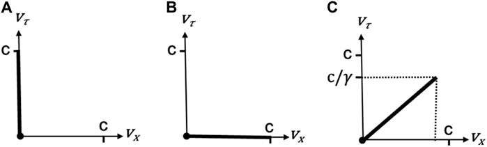
Figure 2. Universal speed constraint visualized as a plot of $v_{\tau }$ vs. $v_x$. Thick solid bar of length c indicates speed magnitude. (A) A particle at rest in frame S’s r-space ($v_x$ = 0, $v_{\tau }=c$). (B) A massless particle such as a photon moving at light speed in frame S’s r-space ($v_x$ = c, $v_{\tau }$ = 0) and not aging. (C) General case of a particle moving in S’s r-space with intermediate speed 0 < $v_x$ < c.

4 Imaginary-valued electromagnetic wave components propagate through time

One can derive from the complex-valued Maxwell’s equations above not only that electromagnetic waves consistent with those of classical electromagnetism exist, but that unlike our current conception of such waves, they propagate into t-space as well as r-space. In other words, the complex-valued equations predict that the imaginary components of electromagnetic waves propagate through time. This is a striking prediction that has no parallel in contemporary electrodynamics and may play an important role in experimentally testing the temporal fields hypothesis, as described in the next section.

To derive a wave equation in a vacuum without charge present, take the reduction curl $\nabla \times$ of Eq. 2.1b’s left side and use Eq. 2.7c to give

$\left(1\right)\nabla \times \left(\nabla \times \mathit{E}\right)=\nabla \left(\nabla \cdot \mathit{E}\right)-{\nabla }^{\mathbf{2}}\mathit{E}=-{\nabla }^2\mathit{E}$

since $\nabla \cdot \mathit{E}=0$ in the absence of charge. Similarly, taking the curl $\nabla \times$ of Eq. 2.1b’s right side results in

$\left(2\right)-\nabla \times \frac{\partial \mathit{B}}{\partial t}=-\frac{\partial }{\partial t}\left(\nabla \times \mathit{B}\right)=-\frac{\partial }{\partial t}\left(\frac{1}{c^2}\frac{\partial \mathit{E}}{\partial t}\right)=-\frac{1}{c^2}\frac{{\partial }^2\mathit{E}}{{\partial t}^2}$

Equating (1) and (2) and carrying out a similar procedure for B starting from Eq. 2.1d gives

$\begin{array}{ccc}{\nabla }^2\mathit{E}=\frac{1}{c^2}\frac{{\partial }^2\mathit{E}}{{\partial t}^2}& \text{and}& {\nabla }^2\mathit{B}=\frac{1}{c^2}\frac{{\partial }^2\mathit{B}}{{\partial t}^2}\end{array}(\mathrm{4.1a,b})$

as complex-valued wave equations that are analogous to those for the original Maxwell equations. Once again equating the real and imaginary parts of these equations gives two sets of wave equations,

$\begin{array}{cc}{\nabla }_x^2{\mathit{E}}_{\mathit{x}}=\frac{1}{c^2}\frac{{\partial }^2{\mathit{E}}_x}{{\partial t}^2}& {\nabla }_x^2{\mathit{B}}_{\mathit{x}}=\frac{1}{c^2}\frac{{\partial }^2{\mathit{B}}_{\mathit{x}}}{{\partial t}^2}\end{array}(\mathrm{4.2a,b})$

and

$\begin{array}{cc}{\nabla }_t^2{\mathit{E}}_{\mathit{t}}=\frac{{\partial }^2{\mathit{E}}_{\mathit{t}}}{{\partial t}^2}& {\nabla }_t^2{\mathit{B}}_{\mathit{t}}=\frac{{\partial }^2{\mathit{B}}_{\mathit{t}}}{{\partial t}^2}\end{array}(\mathrm{4.3a,b})$

The first two of these equations, Eqs. 4.2, are the familiar wave equations for E_x and B_x in empty r-space, where the denominator of the first factor on their right hand sides is the squared speed ${\left|\frac{d\mathit{x}}{dt}\right|}^2$ with which the wave is propagating through r-space, and hence $\left|\frac{d\mathit{x}}{dt}\right|=c$ in m/s. Since velocity ${\mathit{v}}_{\mathit{x}}=\frac{d\mathit{x}}{dt}$, the speed of wave propagation in r-space is $v_x=\left|{\mathit{v}}_{\mathit{x}}\right|=\left|\frac{d\mathit{x}}{dt}\right|=c$ m/s, consistent with what is observed experimentally. The second two equations, Eqs. 4.3, make it explicit that the imaginary portions of electromagnetic waves also propagate through time, not just space. Analogous to the situation in r-space, the first implicit factor on the right hand sides of Eqs. 4.3 is the reciprocal of the squared rate ${\left|\frac{d\mathit{t}}{dt}\right|}^2$ with which the wave is propagating through t-space, and hence $\left|\frac{d\mathit{t}}{dt}\right|=1$ s/s. As defined in Eq. 3.6, in t-space the apparent temporal velocity ${\mathit{v}}_{\mathit{t}}=c\frac{\mathit{d}\mathit{t}}{dt}$ scales this quantity by c, so the speed of wave propagation in t-space is $v_t=\left|{\mathit{v}}_{\mathit{t}}\right|=c\left|\frac{d\mathit{t}}{dt}\right|=c$ m/s, and thus electromagnetic waves also propagate through empty t-space with speed c m/s.

To illustrate a simple solution to the full wave equation Eq. 4.1a in ${\mathbb{C}}^3$, imagine that a single isolated source emits a monochromatic electromagnetic wave pulse (e.g., light) that generates a hyper-spherical wave propagating through r-space and t-space. When sufficiently distant from the source, a portion of this wave can be approximated by a monochromatic sinusoidal plane wave

$\mathit{E}={\mathit{E}}_o{e}^{i\varphi }(4.4)$

in ${\mathbb{C}}^3$, where ${\mathit{E}}_o$ is a constant three dimensional real-valued vector. While plane waves represented in complex exponential form like this are often given as solutions to the standard Maxwell equations in r-space, that is generally done with the understanding that one discards the imaginary part of the solution. In contrast, here we do not discard the imaginary part since complex-valued fields are involved, and we consider the full Eq. 4.4 to be a possible solution. In this solution,

$\varphi =\mathit{k}\cdot \mathit{x}-\mathit{\omega }\cdot \mathit{t}+\delta (4.5)$

is the wave phase, where $\mathit{x}+ic\mathit{t}$ is a point in ${\mathbb{C}}^3$ space, k is a constant spatial wave propagation vector with k = |k| as wave number, $\mathit{\omega }$ is an analogous constant temporal wave propagation vector with $\omega =\left|\mathit{\omega }\right|$ as the wave’s angular frequency, and real valued $\delta$ is a phase constant. Eq. 4.4 represents a solution where the wave fronts in t-space are $\pi /2$ out of phase with those in r-space.

To see that the Eq. 4.4 is a solution to the full wave Eq 4.1a, first substitute ${\mathit{E}}_o{e}^{i\varphi }$ into the left side of Eq. 4.1a, giving

${\nabla }^2\mathit{E}=\left({\nabla }_x^2+i\frac{1}{c^2}{\nabla }_t^2\right){\mathit{E}}_o{e}^{i\varphi }$

$={\mathit{E}}_o\left({\nabla }_x^2\mathit{cos}\varphi +i\frac{1}{c^2}{\nabla }_t^2\mathit{sin}\varphi \right)$

$={\mathit{E}}_o\left({\nabla }_x\cdot {\nabla }_x\mathit{cos}\varphi +i\frac{1}{c^2}{\nabla }_t\cdot {\nabla }_t\mathit{sin}\varphi \right)$

$={\mathit{E}}_o\left(-{\nabla }_x\cdot \mathit{k}\mathit{sin}\varphi -i\frac{1}{c^2}{\nabla }_t\cdot \mathit{\omega }\mathit{cos}\varphi \right)$

$={\mathit{E}}_o\left(-k^2\mathit{cos}\varphi -i\frac{{\omega }^2}{c^2}\mathit{sin}\varphi \right)$

$=-k^2{\mathit{E}}_o{e}^{i\varphi }$

$=-k^2\mathit{E}(4.6)$

where the penultimate step used the relation $k=\omega /c$.

Before substituting ${\mathit{E}}_o{e}^{i\varphi }$ into the right side of Eq. 4.1a to show that it gives the same result as Eq. 4.6, it is helpful to know the derivative $\frac{\partial \varphi }{\partial t}$. To derive this derivative requires the derivative $\frac{\partial \mathit{t}}{\partial t}$ of t-space location vector t with respect to clock time t, constrained by the temporal correspondence $dt=\left|d\mathit{t}\right|$ of Eq. 3.4. To compute $\frac{\partial \mathit{t}}{\partial t}$ under this constraint, note that just as the constant spatial vector k indicates the wave propagation direction in r-space, the constant temporal vector $\mathit{\omega }$ indicates the wave propagation direction in t-space. Let $\widehat{\mathit{\omega }}=\frac{\mathit{\omega }}{\omega }$ be a unit vector pointing in the direction of the wave’s movement in t-space, where $\omega =\left|\mathit{\omega }\right|$. Then over an infinitesimal clock time increment dt, $d\mathit{t}=\widehat{\mathit{\omega }}dt$ due to the temporal correspondence $dt=\left|d\mathit{t}\right|$, giving the needed $\frac{\partial \mathit{t}}{\partial t}=\widehat{\mathit{\omega }}$. It follows that electromagnetic wave speed in t-space in a vacuum is independent of frequency, and that

$\frac{\partial \varphi }{\partial t}=-\frac{\partial }{\partial t}\left(\mathit{\omega }\cdot \mathit{t}\right)=-\mathit{\omega }\cdot \frac{\partial \mathit{t}}{\partial t}=-\mathit{\omega }\cdot \frac{\mathit{\omega }}{\omega }=-\frac{{\omega }^2}{\omega }=-\omega (4.7)$

Thus, substituting ${\mathit{E}}_o{e}^{i\varphi }$ into the right side of Eq. 4.1a results in

$\frac{1}{c^2}\frac{{\partial }^2\mathit{E}}{{\partial t}^2}=\frac{1}{c^2}{\mathit{E}}_o\frac{{\partial }^2}{{\partial t}^2}\left(\mathit{cos}\varphi +i\mathit{sin}\varphi \right)$

$={\frac{\mathbf{1}}{{\mathit{c}}^{\mathbf{2}}}\mathit{E}}_o\frac{\partial }{\partial t}\left(\omega \sin \varphi -i\omega \cos \varphi \right)$

$=\frac{\omega }{c^2}{\mathit{E}}_o\left(-\omega \mathit{cos}\varphi -i\omega \mathit{sin}\varphi \right)$

$=-\frac{{\omega }^2}{c^2}{\mathit{E}}_o\left(\mathit{cos}\varphi +i\mathit{sin}\varphi \right)$

$=-k^2{\mathit{E}}_o{e}^{i\varphi }$

$=-k^2\mathit{E}(4.8)$

where the final steps again used the relation $k=\omega /c$. Since the final quantities in Eqs. (4.8), (4.6) are equal, ${\mathit{E}}_o{e}^{i\varphi }$ is a solution to Eq. 4.1a. Analogous results can be obtained for Eq. 4.1b for B.

Some care is needed in visualizing/interpreting the part of an electromagnetic wave that propagates through t-space because we have no experience directly observing the imaginary-valued part of the wave experimentally. To illustrate this, Figure 3 provides an informal characterization of a wave in a vacuum for an observer o at rest in the r-space of an inertial frame S at the location where a pulse of electromagnetic radiation (e.g., light) is initiated. Cross sections are shown for the r-space and t-space portions of the expanding wave (conceptually a 6D hypersphere in ${\mathbb{C}}^3$) that follows the flash of radiated light at clock time t_a at the origin. While the r-space portion in the top row is familiar and as expected with the observer o remaining at the origin of r-space ($v_x=0$), by the universal speed constraint that same observer is moving through t-space in some direction with speed $v_{\tau }=v_t=c$. Thus, that observer is moving along with a portion of the t-space wave, as pictured in the second row Figure 3 (observer o’s movement through t-space is arbitrarily taken to be in the direction of the dotted arrow) rather than remaining at the origin. While special relativity and Maxwell’s equations indicate that it is impossible for a material object to accelerate so that it can travel along with an electromagnetic wave at speed $v_x=c$ like this in empty r-space, within the theory developed here they also indicate that doing so is commonplace in vacuum t-space. The observer at rest in S’s r-space where the electromagnetic wave is initiated is moving with speed $v_t=c$ in t-space, and thus along with part of the imaginary-valued, unobservable portion of the wave.

Figure 3

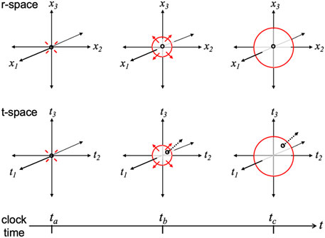
Figure 3. An observer o at rest at the origin of the r-space of an inertial frame S when an electromagnetic wave pulse (e.g., light flash) is initiated there at clock time t_a in a vacuum. Long horizontal black arrow at the bottom indicates passage of clock time t. In the top row, snapshots of the familiar resulting spherical wave in r-space (colored red) are shown at successive times t_b and t_c with o remaining stationary at the origin. In the second row, the same sequence is shown for imaginary valued t-space, but whereas the observer o remains at rest in r-space ($v_x=0$), the universal speed constraint implies that the observer at rest in r-space is moving with speed $v_{\tau }=v_t=c$ in some t-space direction (arbitrarily taken to be along the dotted arrow here) and so o moves along with the wave through t-space as shown.

5 Experimental testing of the hypothesis

Is it possible to falsify experimentally the novel predictions made by the temporal fields hypothesis and the complex-valued Maxwell Eq 2.1? This is a challenging issue, given that electromagnetic fields in t-space are taken a priori to not be directly observable. However, these imaginary-valued fields should be experimentally detectable indirectly based on secondary effects that they cause under special circumstances. Here we consider, as examples, avenues of experimental study that could be pursued to support or to falsify two predictions of the temporal fields hypothesis: demonstrating time dilation for unstable charged particles at rest in r-space, and detecting evidence of imaginary components of electromagnetic waves in dielectrics. Only a brief, qualitative sketch of these two possible approaches is given here–much further thought, analysis, and description of experimental details would be needed to design operational experiments. The only point being made is that, in principle, there are ways to experimentally evaluate the existence of imaginary-valued electromagnetic fields using contemporary experimental methods.

5.1 Time dilation for unstable charged particles at rest

The first experimental approach involves looking for effects of forces exerted on charged particles by the fields B_t and E_t that exist in imaginary-valued t-space. Much of what we know experimentally about the familiar fields E_x and B_x is based on the effects that they exert on matter in r-space. This suggests that we can test the temporal fields hypothesis by analogously looking for effects in time, i.e., in t-space rather than in r-space, on charged matter resulting from forces due to B_t and E_t. For this, we need to first characterize what those forces would be.

In classical electrodynamics, Maxwell’s equations are complemented by the Lorentz force law ${\mathit{F}}_{\mathit{x}}=q_e\left[{\mathit{E}}_{\mathit{x}}+\left({\mathit{v}}_{\mathit{x}}\times {\mathit{B}}_{\mathit{x}}\right)\right]$ describing the force ${\mathit{F}}_{\mathit{x}}$ in r-space due to fields E_x and B_x acting on a particle having electrical charge q_e and moving with velocity v_x through r-space. When hypothesized magnetic charge is considered in the literature as in Eq. 1.2, this law is often extended to be

${\mathit{F}}_{\mathit{x}}=q_e\left[{\mathit{E}}_{\mathit{x}}+\left({\mathit{v}}_{\mathit{x}}\times {\mathit{B}}_{\mathit{x}}\right)\right]+q_m\left[{\mathit{B}}_{\mathit{x}}-\frac{1}{c^2}\left({\mathit{v}}_{\mathit{x}}\times {\mathit{E}}_{\mathit{x}}\right)\right](5.1)$

where forces due to magnetic charge q_m are included [2,3]. This extension is derived from the classic Lorentz force law based on an electromagnetic duality transformation for Eqs. 1.2. Here we proceed analogously, applying the cross-domain duality transformation Eqs. 2.14 to the classic Lorentz force law, which produces

$\mathit{F}={\mathit{F}}_{\mathit{x}}+i{\mathit{F}}_{\mathit{t}}=q\left[{\mathit{E}}_{\mathit{x}}+\left({\mathit{v}}_{\mathit{x}}\times {\mathit{B}}_{\mathit{x}}\right)\right]+icq\left[{\mathit{B}}_{\mathit{t}}-\frac{1}{c^2}\left({\mathit{v}}_{\mathit{t}}\times {\mathit{E}}_{\mathit{t}}\right)\right](5.2)$

The quantity ${\mathit{v}}_{\mathit{x}}=\frac{d\mathit{x}}{dt}$ in the traditional Lorentz force law has been mapped by the cross-domain transformation into $\frac{d\left(c\mathit{t}\right)}{dt}=c\frac{d\mathit{t}}{dt}={\mathit{v}}_{\mathit{t}}$ in the rightmost part of Eq. 5.2. Unlike Eq. 5.1, F in Eq. 5.2 involves forces in both r-space and t-space, q replaces both q_e and q_m, and the forces due to fields B_t and E_t are seen to be purely imaginary valued, extending solely through t-space. Thus, a particle with charge q would be expected to accelerate in r-space according to the traditional Lorentz force law, altering ${\mathit{v}}_{\mathit{x}}$ precisely as we observe, because there is no direct influence on a particle’s movement in r-space due to the B_t and E_t fields. Further, only B_t and E_t would act on a particle’s movement in t-space. For example, a charge q at rest at the origin in r-space produces a field ${\mathit{E}}_{\mathit{x}}=\frac{1}{4\pi {ϵ}_o}\frac{q}{x^2}\widehat{\mathit{x}}$ in electrostatics underlying Coulomb’s Law, where $\widehat{\mathit{x}}$ is a unit vector in the direction of x. Applying the cross-domain duality transformation Eqs. 2.14 to this indicates that

${\mathit{B}}_{\mathit{t}}=\frac{{\mu }_o}{4\pi c}\frac{q}{t^2}\widehat{\mathit{t}}(5.3)$

is a t-space magnetic analog to Coulomb’s law in electrostatics, where $\widehat{\mathit{t}}$ is a unit vector in the direction of another charge in t-space. Thus, in t-space particles of opposite magnetic charge would attract one another, and those with the same magnetic charge would repel one another. These considerations suggest using experimental tests like the following.

Equations Eqs. 5.2, 5.3 predict that under specific circumstances one would observe time dilation affecting the decay rate of unstable charged particles at rest in r-space. In other words, unlike the time dilation effects predicted by special relativity for charged particles moving at relativistic speeds, we are now considering time dilation affecting unstable particles at rest in the r-space of an observer’s reference frame, something predicted to occur by the complex-valued but not by the classic Maxwell equations. As an example, consider a small and very thin hollow spherical shell at rest in the r-space of an observer’s reference frame, as sketched in Figure 4. At an initial time t_i let this shell have fixed, embedded positively charged particles q⁺ in it that are unstable and spontaneously decay with a known half-life when they are at rest (e.g., an ionized radioactive isotope). Suppose that at time t_a a much larger amount q^- of mobile negatively charged stable particles (e.g., electrons) is added to the sphere temporarily, being removed at time t_b. Ignoring transient effects at times t_a and t_b, Eq. 5.3 implies that following time t_b, the dominating negative charge that was present during the period t_a to t_b would result in a strong resultant radial field B_t in t-space pointing towards the shell, as illustrated in Figure 4. By Eq. 5.2, this field would exert a substantial force of c q⁺ B_t on the positively charged particles remaining on the shell following time t_b that would reduce their speed through t-space, and thus reduce the passage of their proper time. This would be manifest experimentally by an apparently increased half-life with slower decay of the unstable positively charged particles between times t_b and t_f. The control experiment for comparison would be the same procedure except without the temporary addition of charge q^- to the sphere during time period t_a to t_b.

Figure 4

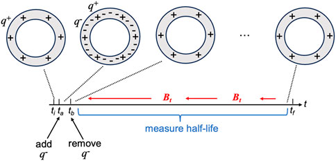
Figure 4. Example sequence of events predicted to produce slowed particle aging (time dilation) via t-space magnetic fields B_t (red arrows). Long horizontal black arrow indicates passage of clock time t. Shown at the upper left at initial time t_i is a maximal cross-section through a thin hollow sphere (thickness not drawn to scale) at rest having fixed embedded unstable particles (q⁺) that are positively charged (+). At time t_a, a much larger amount of mobile stable particles (q^-) that are negatively charged (−) are added, being removed at time t_b, so that the resulting total charge is temporarily strongly negative, thus implying resultant incoming radial fields B_t in t-space as illustrated (red arrows). Decay of the original unstable q⁺ particles during the period from t_b until final time t_f is predicted to be slowed, consistent with a time dilation effect even though they are at rest in r-space.

5.2 Electromagnetic waves in dielectrics

A second potential experimental approach to evaluating the temporal fields hypothesis involves the prediction that the imaginary components of electromagnetic waves propagate through time (t-space). While such waves are not directly observable according to the theory presented here, under special circumstances they may be detectable indirectly because of the universal speed constraint.

The standard Maxwell’s equations are often re-expressed for use inside of matter by introducing an electric displacement vector D and an auxiliary magnetic vector H that capture the macroscopic effects of polarization and magnetization. Taking a similar approach here for the complex-valued Maxwell equations, this would correspond in a homogeneous linear medium to using complex-valued $\mathit{D}=ϵ\mathit{E}$ and $\mathit{H}=\frac{1}{\mu }\mathit{B}$ where $ϵ>{ϵ}_o$ and $\mu >{\mu }_o$ are the medium’s permittivity and permeability, respectively. In the absence of free charge and free current, the complex-valued Maxwell equations inside the medium become

$\begin{array}{cc}\nabla \cdot \mathit{E}=0& \nabla \times \mathit{E}=-\frac{\partial \mathit{B}}{\partial t}\end{array}(\mathrm{5.4a,b})$

$\begin{array}{cc}\nabla \cdot \mathit{B}=0& \nabla \times \mathit{B}=ϵ\mu \frac{\partial \mathit{E}}{\partial t}\end{array}(\mathrm{5.4c,d})$

from which one derives

$\begin{array}{ccc}{\nabla }^2\mathit{E}=ϵ\mu \frac{{\partial }^2\mathit{E}}{{\partial t}^2}& \text{and}& {\nabla }^2\mathit{B}=ϵ\mu \frac{{\partial }^2\mathit{B}}{{\partial t}^2}\end{array}(\mathrm{5.5a,b})$

as complex-valued wave equations. These are the same as the vacuum wave equations 4.1 except that $\frac{1}{c^2}={ϵ}_o{\mu }_o$ has been replaced by $ϵ\mu$.

Equating the real and imaginary parts of these equations gives two sets of wave equations,

$\begin{array}{ccc}{\nabla }_x^2{\mathit{E}}_{\mathit{x}}=ϵ\mu \frac{{\partial }^2{\mathit{E}}_x}{{\partial t}^2}& \text{and}& {\nabla }_x^2{\mathit{B}}_{\mathit{x}}=ϵ\mu \frac{{\partial }^2{\mathit{B}}_{\mathit{x}}}{{\partial t}^2}\end{array}(\mathrm{5.6a,b})$

and

$\begin{array}{ccc}{\nabla }_t^2{\mathit{E}}_{\mathit{t}}=ϵ\mu c^2\frac{{\partial }^2{\mathit{E}}_{\mathit{t}}}{{\partial t}^2}& \text{and}& {\nabla }_t^2{\mathit{B}}_{\mathit{t}}=ϵ\mu c^2\frac{{\partial }^2{\mathit{B}}_{\mathit{t}}}{{\partial t}^2}\end{array}(\mathrm{5.7a,b})$

in r-space and imaginary-valued t-space, respectively. It follows from an analysis similar to that of Sect. 4 that wave speed inside the medium is

$v_x=v_t=\frac{1}{\sqrt{ϵ\mu }}=\frac{c}{n}(5.8)$

where $n=\sqrt{\frac{ϵ\mu }{{ϵ}_o{\mu }_o}}$ is the medium’s index of refraction.

Consider the observable portion of a planar electromagnetic wave that is initially traveling through vacuum with speed $v_x=c$ in the r-space of an inertial reference frame S. According to the universal speed constraint Eq. 3.17, the photons in that wave are traveling at speed $v_{\tau }=0$ through S’s t-space and thus are not aging. When this wave is normally incident upon a dielectric material at rest in S that is substantially transparent at the wave’s frequency, the transmitted portion of the wave’s speed through the dielectric decreases to $v_x=c/n$. In this situation the universal speed constraint implies that for the photons comprising the wave,

$v_{\tau }^2=c^2-v_x^2=c^2-\frac{1}{n^2}{c}^2=c^2\left(1-\frac{1}{n^2}\right)>0(5.9)$

must hold, and thus these photons in the wave inside the dielectric are aging, unlike with a wave moving through a vacuum, but it is unclear how this could be experimentally verified.

On the other hand, consider a portion of a wave initiated inside of a sphere of dielectric material that is traveling inside the dielectric in the same direction through t-space as the dielectric material. By Eq. 5.8, the photons in this portion of the wave would have a speed of $v_{\tau }=c/n$. It follows from Eq. 3.17 that for these photons,

$v_x^2=c^2-v_{\tau }^2=c^2-\frac{1}{n^2}{c}^2=c^2\left(1-\frac{1}{n^2}\right)(5.10)$

must hold. Thus, unlike in a vacuum t-space, photons comprising this portion of the wave would “spill over” into r-space, and thus they would be potentially detectable as they exit the dielectric. These considerations suggest experimental tests such as the following.

Consider a solid sphere of homogeneous linear dielectric material having a refractive index of $n$ > 1 at rest in reference frame S (Figure 5). Let there be a very short burst of electromagnetic radiation at the center of the sphere at a frequency at which the dielectric is largely transparent. In r-space, the observable part of the wave rapidly weakens due to attenuation and to transmission outside of the block at the boundaries (Figure 5, left side). For example, for light in a typical glass sphere ($n\approx 1.5$) surrounded by air/vacuum, only 4% of the wave’s energy remains in the sphere after just the first reflection. The imaginary-valued portion of the wave inside the dielectric sphere that is moving in the same direction in t-space as the block (see Figure 3) does not directly experience losses from transmission outside the block because it does not encounter these r-space boundaries (Figure 5, right side). However, because the photons in this part of the wave have speed $v_{\tau }=\frac{c}{n}<c$ inside the dielectric, by the universal speed constraint and by Eq. 5.10 they must also have speed $v_x=c{\left(1-\frac{1}{n^2}\right)}^{1/2}>0$ there. Thus, the temporal fields hypothesis predicts that these persistent r-space electromagnetic waves will be transmitted through the block’s boundaries for a substantially longer time period beyond what would be predicted by the classic Maxwell equations. Such r-space waves, although perhaps quite weak, should be detectable by a nearby observer at rest in r-space. To be maximally informative, variations of such an experiment could be done using materials with different n values, waves of different frequencies (e.g., from ELF to visible), etc.

Figure 5

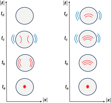
Figure 5. Snapshots of events following a very short burst of electromagnetic radiation occurring at clock time t_a, located at the center of a solid sphere of dielectric material (black circles) that is at rest in the r-space of frame S and is surrounded by vacuum/air. The waves have a frequency for which the dielectric is largely transparent. As shown on the left, in r-space the spherical wave (vertical red arcs) propagates in all three dimensions (t_b), with some of the wave being transmitted (blue arcs) and some being reflected (red arcs) at the boundaries (t_c). The r-space wave inside the dielectric quickly vanishes (t_d) due to both repeated transmission through the boundary and attenuation. In contrast, on the right an imaginary-valued portion of the same wave is shown inside the dielectric material (horizontal red arcs) moving in the same direction through t-space as the sphere. This specific t-space portion of the wave inside the dielectric does not encounter boundaries, so it is not weakened by transmission losses at the boundaries of the dielectric as occurs in r-space. However, its reduced $v_{\tau }<c$ through t-space in the dielectric implies that it must spill over into r-space, producing an r-space part of the wave (blue arcs) which persists for a longer time period than is predicted by the standard Maxwell equations.

6 Discussion

In classical electrodynamics, the fields E and B are assumed to extend solely into three dimensional space (r-space) and thus to have three real-valued components. In contrast, the work presented here has asked what the consequences would be if these fields actually have three complex-valued components where the unobservable imaginary parts extend into three dimensional time (t-space) rather than space. The approach taken here to addressing this issue is driven by maximizing the symmetry of Maxwell’s equations. The resulting complex-valued Maxwell equations are more symmetrical than the classic Maxwell equations in multiple ways: both electric charge and magnetic charge exist, these types of charge are the same entity, both space and time are three dimensional, and the fields extend into both space and time (Table 1). In spite of these generalizations, the complex-valued Maxwell equations remain consistent with the originals and with the existing experimental results of classical electromagnetism.

An interesting aspect of the complex-valued Maxwell equations considered here is what they imply about the nature of time. There is a very large literature in physics, psychology, neuroscience, and philosophy with widely divergent views about time; for example, [26, 38–42]. Opinions differ regarding such fundamental issues as whether or not the concept of time is an illusion, whether or not the past and future always exist (block vs. dynamic Universe, eternalists vs. presentists, etc.), what the relationship is between objective physical time and human subjective time (flow of time, concept of Now, etc.), and what determines the arrow of time (thermodynamic, cosmological, electromagnetic, etc.). The hypothesis that electromagnetic fields have three separate imaginary-valued components extending into time contributes to this discussion by implying that in some sense a separate, unobservable 3D temporal space underlies our familiar concept of objective clock time. This is captured in the theory by identifying a temporal correspondence equating the amount of clock time that we measure between two events to the extent that those events are separated in the underlying t-space (Eq. 3.4). A resting clock having periodic cycles that mark the distance traversed in t-space regardless of the direction of movement thus becomes completely analogous to a resting ruler having periodic lines that mark the distance traversed in r-space regardless of the direction of movement.

Two very striking predictions follow from the temporal fields hypothesis that are not predicted by the standard Maxwell equations. First, the complex-valued Maxwell equations imply that electrically charged particles also serve as magnetic monopoles having magnetic fields extending into t-space. Such magnetic monopoles would not be detected by current search methods because they do not have magnetic fields extending into r-space. The second striking prediction is that electromagnetic waves not only propagate through space but also through time. Surprisingly, portions of these unobservable waves travel through vacuum t-space at the same speed as observers at rest in an inertial reference frame S. This unanticipated result implies that an observer at rest in frame S would be traveling through t-space along with a wave front generated at the observer’s location, something that is forbidden by special relativity in r-space. This prediction follows from the temporal fields hypothesis based on a straightforward derivation of the wave equation from the complex-valued Maxwell equations, and from the invariance of the complex spacetime interval under a Lorentz transformation in ${\mathbb{C}}^3$. If the temporal fields hypothesis proves to be correct, information could thus be transmitted through time in a previously unsuspected fashion, and this could have important scientific and technological implications.

The theoretical work presented here provides only some initial steps towards characterizing the implications of the temporal fields hypothesis. It has some significant limitations, as follows. As noted in the Introduction, this work only considers classical electrodynamics in flat spacetime. Incorporating considerations of cosmology, such as the implications of introducing curved spacetime and general relativity, would be of substantial interest. For example, are closed time-like loops possible in 3D t-space, and if so, would they affect our experienced conventional 4D spacetime based on measured clock time t, disrupting causality in some fashion (see Footnote 1)? Does the extension of electromagnetic fields to t-space have any implications for understanding the nature of dark energy/matter or the possible existence of a “fifth force”? Further, extending the current hypothesis to quantum physics also raises many issues and would be an extremely important next step in theory development. Would quantification of the fields lead to any new and unexpected results? Would they contribute to our understanding of entanglement (e.g., particles widely separated in r-space but still close in t-space)? Would fields extending into time provide a different interpretation of what virtual photons are or new insights into their role in the Casimir effect? How would the existence of electromagnetic waves in t-space relate to non-propagating evanescent waves involving virtual photons, and to the nature of the underlying energy source harvested by recently invented devices that extract electric power from the zero-point energy associated with quantum vacuum fluctuations [44]?

Even within classical electrodynamics there are substantial limitations to what has been done so far. Complex scalar and vector potentials need to be introduced, something that is complicated by the cross-domain duality (e.g., in contrast to in r-space, a scalar potential is needed for B_t while a vector potential is needed for E_t). In addition, energy considerations need to be analyzed, similar to the energy conservation analysis that was done previously [4] for the complex Maxwell equations that had imaginary components in space rather than in time as is the case here. Finally, while the possible experimental tests of the hypothesis described in Section 5 are intended only to show in principle that there are ways to test the hypothesis, those tests will need to be fleshed out in quantitative detail to be realizable. In the current absence of direct experimental data characterizing attenuation of the field imaginary components, this is tremendous challenge whose resolution depends on the materials used, what their properties are in t-space (e.g., rate of wave attenuation in t-space, given that charge does not have an imaginary component as described in the first paragraph of Section 2.2), selecting appropriate frequencies to test, etc. These issues might be resolved in part by systematic exploratory finite-element simulations that solve for real and imaginary field components over a broad range of possibilities. All of these limitations represent important directions for possible future work, which might also include simplifying and illuminating the analysis done here by repeating it using a Clifford algebra [45].

While challenging, experimental tests of the temporal fields hypothesis are clearly merited because of the potential impact on our understanding of electromagnetism and spacetime physics. Finding experimental evidence that electromagnetic fields have components extending into t-space, using methods like those discussed above or other approaches, could ultimately have tremendous implications for the foundations of physics. Even if experimental evaluation should fail to find support for the existence of imaginary-valued field components, then such results will still be interesting, because they would indicate the need for a theoretical explanation of why, in the unified spacetime that underlies contemporary physics, electromagnetic fields do not extend into the temporal aspects of spacetime. In other words, if space and time are truly integrated in the way existing theory indicates, then why do electromagnetic fields extend only into space and not into time? To the author’s knowledge this latter issue has not been substantially considered previously.

Data availability statement

The original contributions presented in the study are included in the article/Supplementary material, further inquiries can be directed to the corresponding author.

Author contributions

JR: Conceptualization, Formal Analysis, Investigation, Methodology, Project administration, Visualization, Writing–original draft, Writing–review and editing.

Funding

The author(s) declare that no financial support was received for the research, authorship, and/or publication of this article.

Acknowledgments

The author thanks the reviewers for their substantial constructive comments.

Conflict of interest

The author declares that the research was conducted in the absence of any commercial or financial relationships that could be construed as a potential conflict of interest.

Publisher’s note

All claims expressed in this article are solely those of the authors and do not necessarily represent those of their affiliated organizations, or those of the publisher, the editors and the reviewers. Any product that may be evaluated in this article, or claim that may be made by its manufacturer, is not guaranteed or endorsed by the publisher.

Footnotes

¹Multidimensional time raises the issue of whether closed time-like loops might be possible in flat spacetime. Here it is simply assumed that such closed curves do not occur in 3D t-space, but this needs further analysis. Even if they are possible, the temporal correspondence of Eq. 3.4 implies that there would not be a closed loop involving measurable clock time t, and thus no disruption of causality as we experience it.

References

1. Frisch M. Inconsistency, asymmetry, and non-locality. Oxford, United Kingdom: Oxford University Press (2005).

Google Scholar

2. Griffiths D. Introduction to electrodynamics. Cambridge, United Kingdom: Cambridge University Press (2017).

Google Scholar

3. Zangwill A. Modern electrodynamics. Cambridge, United Kingdom: Cambridge University Press (2013).

Google Scholar

4. Reggia J. Generalizing Maxwell’s equations to complex-valued electromagnetic fields. Physica Scripta (2024) 99(1):015513. doi:10.1088/1402-4896/ad10dc

CrossRef Full Text | Google Scholar

5. Gonano C, Zich R. Magnetic monopoles and Maxwell’s equations in N dimensions. In: International Conference on Electromagnetics in Advanced Applications; September, 2013; Turin, Italy (2013). p. 1544–7.

Google Scholar

6. Keller O. Electrodynamics with magnetic monopoles: photon wave mechanical theory. Phys Rev A (2018) 98:052112. doi:10.1103/physreva.98.052112

CrossRef Full Text | Google Scholar

7. Schwinger J. A magnetic model of matter. Science (1969) 165:757–61. doi:10.1126/science.165.3895.757

PubMed Abstract | CrossRef Full Text | Google Scholar

8. Acharya B, Alexandre J, Benes P, Bergmann B, Bernabéu J, Bevan A, et al. First search for dyons with the full MoEDAL trapping detector in 13 TeV pp collisions. Phys Rev Lett (2021) 126:071801. doi:10.1103/physrevlett.126.071801

PubMed Abstract | CrossRef Full Text | Google Scholar

9. McDavid A, McMullen C. Generalizing cross products and Maxwell’s equations to universal extra dimensions (2006). Available from: http://arxiv.org/ftp/hep-ph/papers/0609/0609260.pdf (Accessed May 28, 2024)

Google Scholar

10. Weinreich G. Geometrical vectors. Chicago, USA: University of Chicago Press (1998).

Google Scholar

11. Bialynicki-Birula I. On the wave function of the photon. Acta Physica Pol A (1994) 86:97–116. doi:10.12693/aphyspola.86.97

CrossRef Full Text | Google Scholar

12. Mohr P. Solutions of the Maxwell equations and photon wave functions. Ann Phys (2010) 325:607–63. doi:10.1016/j.aop.2009.11.007

CrossRef Full Text | Google Scholar

13. Arbab A. Complex Maxwell’s equations. Chin Phys B (2013) 22:030301–6. doi:10.1088/1674-1056/22/3/030301

CrossRef Full Text | Google Scholar

14. Aste A. Complex representation theory of the electromagnetic field. J Geometry Symmetry Phys (2012) 28:47–58. doi:10.7546/jgsp-28-2012-47-58

CrossRef Full Text | Google Scholar

15. Livadiotis G. Complex symmetric formulation of Maxwell’s equations for fields and potentials. Mathematics (2018) 6(114):1–10. doi:10.3390/math6070114

CrossRef Full Text | Google Scholar

16. Salih M. Complex Maxwell equations. J Mod Phys (2023) 14:1662–71. doi:10.4236/jmp.2023.1412097

CrossRef Full Text | Google Scholar

17. Mavromatos N, Mitsou V. Magnetic monopoles revisited: models and searches at colliders and in the Cosmos. Int J Mod Phys A (2020) 35(2020):2030012. doi:10.1142/s0217751x20300124

CrossRef Full Text | Google Scholar

18. Dirac P. Quantized singularities in the electromagnetic field. Proc R Soc Lond A (1931) 133:60–72. doi:10.1098/rspa.1931.0130

CrossRef Full Text | Google Scholar

19. T’t Hooft G. Magnetic monopoles in unified gauge theories. Nucl Phys B (1974) 79:276–84. doi:10.1016/0550-3213(74)90486-6

CrossRef Full Text | Google Scholar

20. Polyakov A. Particle spectrum in the quantum field theory. JETP Lett (1974) 20:194–5. doi:10.1142/9789814317344_0061

CrossRef Full Text | Google Scholar

21. Wu T, Yang C. Concept of nonintegrable phase factors and global formulation of gauge fields. Phys Rev D (1975) 12:3845–57. doi:10.1103/physrevd.12.3845

CrossRef Full Text | Google Scholar

22. Singleton D. Magnetic charge as a hidden gauge symmetry. Int J Theor Phys (1995) 34:37–46. doi:10.1007/bf00670985

CrossRef Full Text | Google Scholar

23. Singleton D. Electromagnetism with magnetic charge and two photons. Am J Phys (1996) 64:452–8. doi:10.1119/1.18191

CrossRef Full Text | Google Scholar

24. Ho D, Rajantie A. Instanton solution for schwinger production of ’t hooft–polyakov monopoles. Phys Rev D (2021) 103:115033. doi:10.1103/physrevd.103.115033

CrossRef Full Text | Google Scholar

25. Lazarides G, Shafi Q. Electroweak monopoles and magnetic dumbbells in grand unified theories. Phys Rev D (2021) 103:095021. doi:10.1103/physrevd.103.095021

CrossRef Full Text | Google Scholar

26. Arstila V, Lloyd D. Subjective time. Cambridge, Massachusetts, United States: MIT Press (2014).

Google Scholar

27. Maccarrone G, Recami E. Revisiting the superluminal Lorentz transformations and their group theoretical properties. Lettere al Nuovo Cimento (1982) 34:251–6. doi:10.1007/bf02817120

CrossRef Full Text | Google Scholar

28. Cole E. Generation of new electromagnetic fields in six-dimensional special relativity. Il Nuovo Cimento (1985) 85B:105–17. doi:10.1007/bf02721524

CrossRef Full Text | Google Scholar

29. Haug E. Three dimensional space-time gravitational metric, 3 space + 3 time dimensions. J High Energ Phys Gravitation Cosmology (2021) 7:1230–54. doi:10.4236/jhepgc.2021.74074

CrossRef Full Text | Google Scholar

30. Dattoli G, Mignani R. Formulation of electromagnetism in a six dimensional space-time. Lettere al Nuovo Cimento (1978) 22:65–8. doi:10.1007/bf02786138

CrossRef Full Text | Google Scholar

31. Taylor J. Do electroweak interactions imply six extra time dimensions. J Phys A (1980) 13:1861–6. doi:10.1088/0305-4470/13/5/044

CrossRef Full Text | Google Scholar

32. Bars I. Two-time physics in field theory. Phys Rev D (2000) 62:046007. doi:10.1103/physrevd.62.046007

CrossRef Full Text | Google Scholar

33. Bars I. Gauge symmetries in phase space. Int J Mod Phys A (2010) 25:5235–52. doi:10.1142/9789814335614_0026

CrossRef Full Text | Google Scholar

34. Medina M, Nieto J, Nieto-Marin P. Cosmological duality in four time and four space dimensions. J Mod Phys (2021) 12:1027–39. doi:10.4236/jmp.2021.127064

CrossRef Full Text | Google Scholar

35. Lanciani P. A model of the electron in a 6-dimensional spacetime. Foundations Phys (1999) 29:251–65. doi:10.1023/A:1018825722778

CrossRef Full Text | Google Scholar

36. Nieto J, Espinoza M. Dirac equation in four time and four space dimensions. Int J Geometric Methods Mod Phys (2017) 14:1750014. Article 1750014. doi:10.1142/s0219887817500141

CrossRef Full Text | Google Scholar

37. Martínez-Olivas B, Nieto J, Sandoval-Rodríguez A. (4 + 4)-dimensional space-time as a dual scenario for quantum gravity and dark matter. J Appl Math Phys (2022) 10:688–702. doi:10.4236/jamp.2022.103049

CrossRef Full Text | Google Scholar

38. Buccheri R, Saniga M, Stuckey W. The nature of time: geometry, physics and perception. London, UK: Kluwer Academic (2003).

Google Scholar

39. Majid S. On space and time. Cambridge, United Kingdom: Cambridge University Press (2008).

Google Scholar

40. Muller R. The physics of time. New York, New York, United States: Norton (2016).

Google Scholar

41. Musser G. Putting ourselves back in the equation. Strus and Giroux: Farrar (2023).

Google Scholar

42. Weinert F. The march of time – evolving conceptions of time in the light of scientific discoveries. Berlin, Germany: Springer (2013).

Google Scholar

43. Mermin N. It’s about Time. Princeton, New Jersey, United States: Princeton University Press (2005).

Google Scholar

44. Moddel G. Zero-point energy: capturing evanescence. J Scientific Exploration (2022) 36:493–503. doi:10.31275/20222567

CrossRef Full Text | Google Scholar

45. Jancewicz B. Multivectors and Clifford algebra in electrodynamics. World Scientific (1989). doi:10.1142/0419

CrossRef Full Text | Google Scholar