- 1Complex Systems Research Center, Shanxi University, Taiyuan, China
- 2Department of Mathematics, Saveetha School of Engineering SIMATS, Chennai, India
- 3Department of Mathematics, Kwame Nkrumah University of Science and Technology, Kumasi, Ghana
The spread and control of coronavirus disease 2019 (COVID-19) present a worldwide economic and medical burden to public health. It is imperative to probe the effect of vaccination and infectivity reductions in minimizing the impact of COVID-19. Therefore, we analyze a mathematical model incorporating different infectivity reductions. This work provides the most economical and effective control methods for reducing the impact of COVID-19. Using data from Ghana as a sample size, we study the sensitivity of the parameters to estimate the contributions of the transmission routes to the effective reproduction number
1 Introduction
Coronavirus disease 2019 (COVID-19) is one of the infectious diseases that has caused a global medical and financial burden. Due to its high transmission rate, the World Health Organization (WHO) officially announced the prevalence of it as a global pandemic on 8th March 2020. The coronavirus spreads directly or indirectly from one infectious living host cell to another by replicating and causing infectious disease in the host (humans and/or animals) [1]. Therefore, it is imperative to investigate how the virus spreads in the community and devise strategies to halt the disease’s transmission.
Globally, COVID-19 has caused over 6 million deaths, and by March 2022, approximately 480 million incidences had been reported, according to [2]. However, the COVID-19 reinfection scenario using the SIR model shows that transmission dynamics could arise as a result of immunity waning, even in cases where the force of reinfection is relatively weak [3]. As mentioned in [4], the COVID-19 model, which entails infection through objects contaminated with SARS-CoV-2, is suggested to be made public knowledge.
COVID-19 spreads quickly, threatening global health and igniting a pandemic. This pandemic has had a major effect on other sectors, especially the socioeconomic sector [5]. As of 30 April 2022, there were 512,466,045 reported incidences and 6,257,512 COVID-19 fatalities worldwide, according to the Worldometer. With 6,046,467 COVID-19 cases reported overall, Indonesia ranks seventh in Asia and 18th globally [6].
These findings highlight the need to investigate the spread of COVID-19 in order to minimize its transmission. Using a deterministic model is one way that mathematics is crucial to simulating the epidemic phenomenon of the disease’s spread. The analysis of the COVID-19 model with declining immunity has advanced significantly. For the latter, the natural immunity period is defined by the vaccine efficacy level, which dictates when to start the mass vaccination strategy based on models involving symptomatic and asymptomatic infected populations, as explained in [6].
Mathematical models have been an important tool in epidemiology since the 18th century and can be used to determine the level of spread of infectious disease, aside from medical and biological research studies and strategies for controlling diseases. A modified susceptible–exposed–infectious–removed (SEIR) model with vaccination, quarantine, and isolated SVEQIMR is used to analyze the spread of COVID-19 disease in [7]. In this article, compartmental models were used to demonstrate the pattern of vaccination and control strategies for infectious diseases.
Furthermore, the compartmental model is used to study the behavior of COVID-19 after the introduction of vaccines in [8]. In this article, the population is divided into distinct compartments to demonstrate the control efficacy of infectious diseases in India. Again, a parameterized nonlinear SEIHR model to analyze the transmission of coronavirus disease in Indonesia using the compartmental model is analyzed in [9].
The transmission dynamics, basic reproduction number, and control measures of COVID-19 are analyzed using the compartmental model in [10]. In this article, effective public health interventions were proposed to control the spread of the disease in Wuhan, China. The cost-effective analysis, global stability, and control strategy for the spread of COVID-19 in Ghana are analyzed using the compartmental model in [11]. In this article, control measures were outlined by formulating the SEAIRV model to investigate human–environment–human transmission. However, these studies do not capture the effects of reducing the infectivity rate on the disease’s transmission.
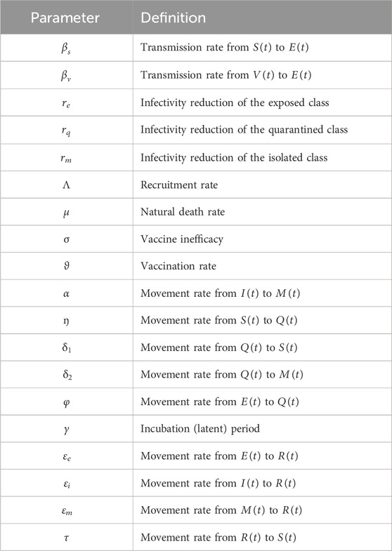
The aforementioned issues have driven this study to explore the effects of vaccination and infectivity reductions on the spread of COVID-19, devise optimal control interventions, and analyze the cost–benefits of implementing the interventions. The subsequent sections are as follows: in Section 2, we present the design of the epidemiological model together with the definition of the parameters and variables in the model. In Section 3, we analyze the positivity of the model’s solutions, computation of the models’ reproduction numbers, and stability of the model. In Section 4, we present the model parameter estimation and sensitivity analysis. In Section 5, we present the numerical simulations and model analysis. In Section 6, we present the optimal control strategies and analyze the cost–benefit analysis. We finally present the concluding remarks of this study in Section 7.
2
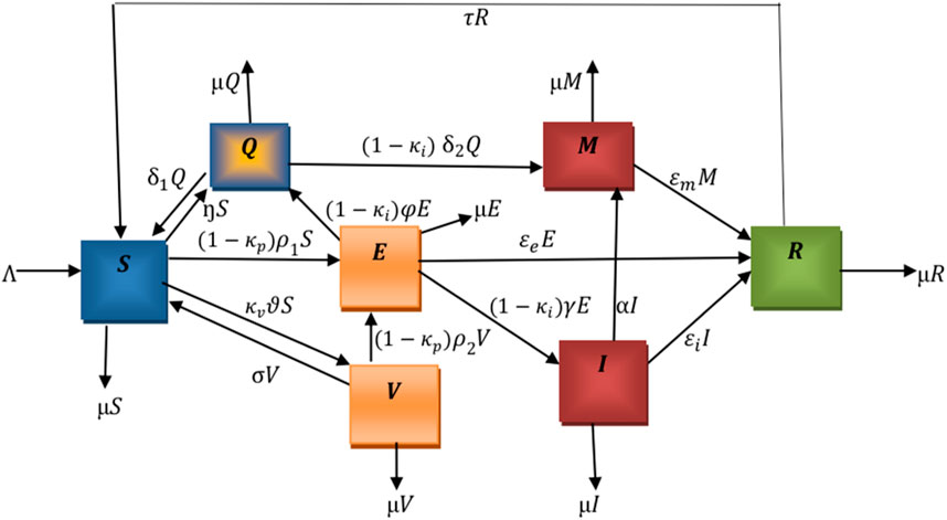
The flowchart below illustrates the mechanism of the model. We denote
The total population
The following nonlinear ordinary differential equations illustrate the model.
where
With initial conditions
3
The detailed analysis of the model is conducted mathematically to show the positivity of solutions and their boundedness within a specific domain.
3.1 Positivity and boundedness of solutions
The variables and parameters of model (2) are nonnegative since it is based on a population with COVID-19.
Theorem 1. Define
Proof: Let us consider the following instance where there exists an initial time
Here,
Therefore,
This contradicts the claim
Theorem 2. To prove the boundedness of model (2), define a positive invariant set as
Proof: Considering Eq. 1.
The rate of change in the total population is given as
From Eq. (3), it follows that,
Then,
3.2 Disease-free equilibrium and effective reproduction number
The disease equilibrium point,
At disease-free equilibrium (DFE), we set
At disease-free equilibrium,
The corresponding Jacobian matrix of the system (2) evaluated at
where
Using
where
The effective reproduction number,
where
Substituting
Therefore, there is a unique equilibrium in the model, which implies that
• In the absence of vaccination, the reproduction number,
• In the absence of infectivity reductions, the reproduction number,
• In the absence of vaccination and infectivity reductions, the reproduction number,
3.3 Stability analysis
Next, since the system has unique equilibrium points, we check its stability.
3.4 Local stability of disease-free equilibrium
The Jacobian matrix,
where
Therefore, the remaining eigenvalues are the roots of the following characteristic polynomial:
where
Therefore, using the Routh–Hurwitz stability conditions, the roots of
3.5 Existence of endemic equilibrium of the model
Let us consider
where
Then,
Substituting the expressions for
Simplifying the above equation gives Eq. (16)
where
Note that, in evaluating
Substituting
Let
It follows that
The expressions for
Let us consider the denominators of
(a) If
(b) If
Using Eq. (17), for
3.6 Global stability of endemic equilibrium
Let us consider a globally positively definite and unbounded function
Theorem 3. The system (14) has an endemic equilibrium
Proof. We define the Lyapunov function
from Eq. (19), we have
Substituting (2) and (18) into (20) gives
Solving the (21) value gives
Let
Hence, the result is
From the above Eqs (22, 23), it can be realized that if the arithmetic mean is greater than or equal to their geometric mean, then
4 Model parameterization and sensitivity analysis
We evaluate the reproduction number to find the transmission routes of the pandemic and the proportion of individuals. A sensitivity analysis was carried out to evaluate the contribution of each parameter to the reproduction number.
4.1 Estimation of model parameters
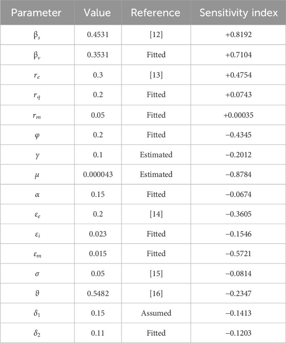
We evaluate the reproduction numbers using the values in Table 3. The effective reproduction number
Table 2 reveals that the infectious and exposed classes contribute significantly to the transmission of the disease. This implies that there must be admissible measures to halt the transmission of the disease.
4.2 Sensitivity analysis
We illustrate the arithmetic behavior of model (2) parameters’ sensitivity. The sensitivity of the parameters in
where
From the above analysis, it is observed that
Based on the numerical illustrations shown in Table 3, the effective reproduction number
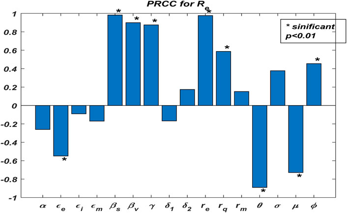
Now, we examine the relationship between the parameters of effective reproduction number
From Figure 2, one could realize that
4.3 Effects of vaccination and infectivity reductions on the effective reproduction number
This subsection explores the dynamics of
Figure 3A demonstrates the influence of vaccination rate
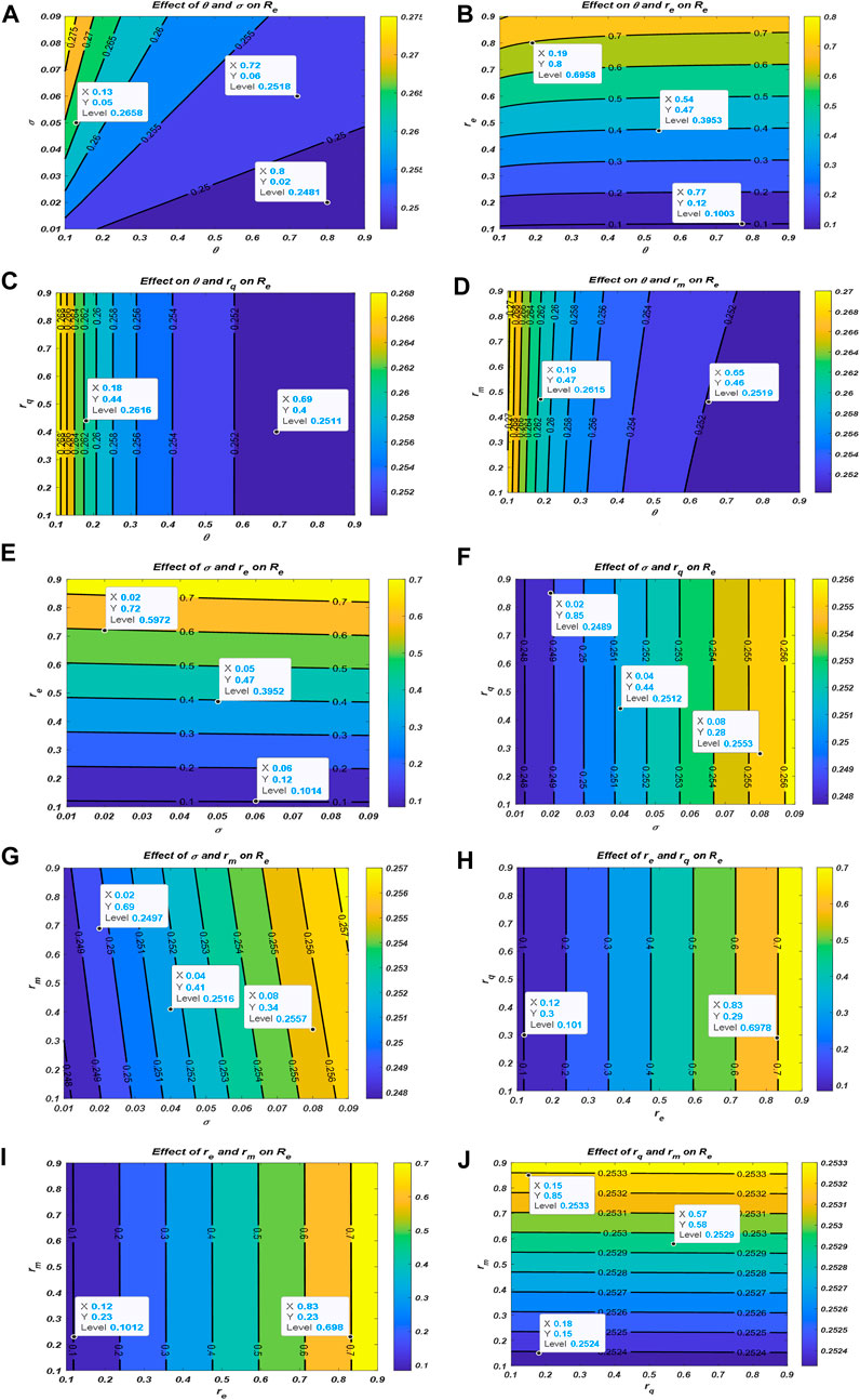
Figure 3. Effect of vaccination and infectivity reductions on the effective reproduction number
5 Numerical simulations and discussions
In this section, the real data are observed to depict the situation of the transmission. The real data are compared with the model’s solution accuracy. The proposed model is applied to explore the transmission of COVID-19 disease in Ghana using data from the WHO [17]. This includes the daily number of infections and the total number of daily infections after the introduction of vaccines. The data are analyzed and compared to other literature works for the simulations. The daily infections and the total number of infections are simulated to analyze the behavioral pattern of the transmission of the disease. In particular, we illustrate the changing effects of the vaccination rate
5.1 Application of the
Once the model is formulated, it is necessary to compare it with data to check its validity. Here, we want to check the accuracy and authenticity of the model by verifying the extent to which the model can represent the real situation, as described in [18]. The simulation consists of the application of the data from Ghana to illustrate the transmission of COVID-19 for the period 1st January 2022 to 1st March 2022 when the individuals were vaccinated. The following state variables are considered using data from Ghana for the period 1st January 2022 to 1st March 2022 [17]. The estimated total population of Ghana is
The SVEQIMR model (fitted) depicts the pattern of the real situation (real data), as shown in Figure 4A, which represents the plot of the daily number of infections, and Figure 4B represents the total number of infections for the period of 1st January 2022 to 1st March 2022. The plot of the model results indicates the pattern of the real situation. That is, the fitted model and real situation agree with each other and illustrate the transmission dynamics of the spread of the pandemic.

Figure 4. Plot of (A) the daily cases and (B) the total number of cases of the fitted model verses the real data from 1st January to 1st March 2022.
5.2 Effects of vaccination and infectivity reductions on COVID-19 incidences
Here, we analyze the influence of vaccination rate and vaccine inefficacy on the spread of COVID-19 disease using the same dataset. Let us consider the following parameters: vaccination rates
Again, we demonstrate the changing effects of the different infectivity reductions on the behavioral pattern of the transmission of COVID-19 disease by considering the following arbitrary values
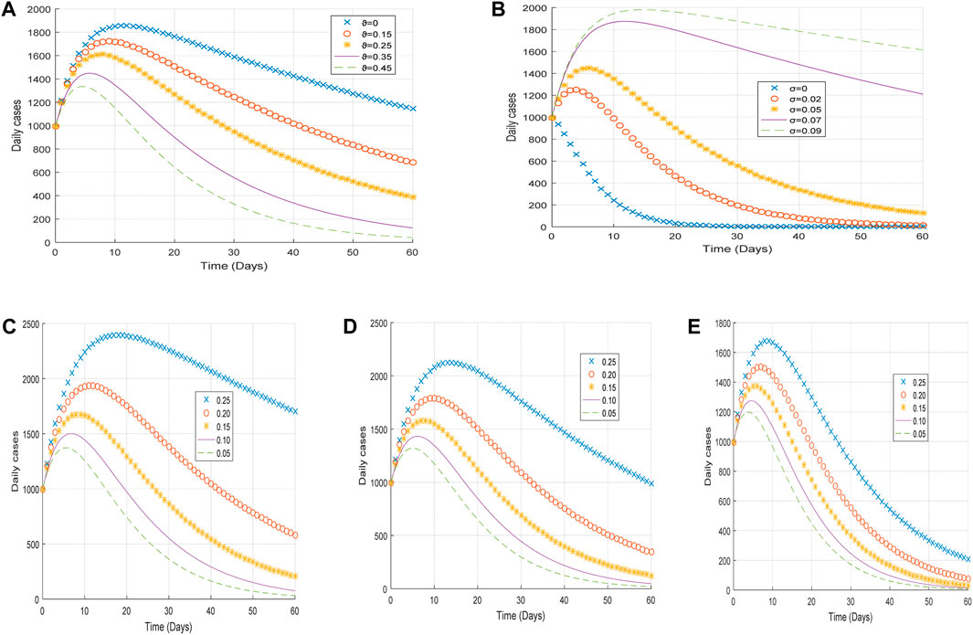
Figure 5. Plot of (A) the impact of vaccination rate
From Figure 5A, it is observed that an increase in the vaccination rate
From Figure 5C, it is realized that an increase in the infectivity reduction of exposed individuals
6 Optimal control problem and cost–benefit analysis
We modify Equation 2 with the following optimal control variables:
where
6.1 Objective functional
We now formulate the optimal trajectories that show the effect of the control efforts
We focus on minimizing the cost function (26), and the total cost of implementing the optimal control is given as
The parameters
Now, we establish point-wise Hamiltonian
where
Theorem 4. Given
with conditions
Proof: We formulate the adjoint equation for the optimal system by taking the partial derivative of Eq. 30 as follows in Eq. (32):
The control set illustrates the co-state system with the optimal conditions.
We solve for
Therefore, using the bounds of the controls
6.2 Optimal control strategies
Here, our aim is to determine the number of infections after deploying the optimal control interventions. We explore the effects of implementing the interventions; therefore, the optimality system (36) is solved forward in time and the adjoint system backward in time with the corresponding lower and upper bounds of the controls. We used the population of Ghana to study the behavioral pattern of COVID-19. The estimated total population of Ghana is
6.2.1 Strategy 1: implementation of public awareness (
The optimal solutions illustrated in Figure 6 account for the observations when the control effort

Figure 6. Optimal solutions of implementing strategy 1. Plot (A) blue dotted line is the optimal solution for implementing strategy 1. (B) Optimal control profile for strategy 1.
The optimal solutions illustrated above depict the following observations when public education is only applied:
(a) Figure 6A represents the effect of the control effort
(b) Figure 6B represents the profile of the control effort for public awareness of COVID-19. It implies that education on COVID-19 should reach 50% of the population throughout the implementation to halt COVID-19 transmission.
6.2.2 Strategy 2: implementation of vaccination (
The optimal solutions illustrated in Figure 7 account for the observations when the control effort
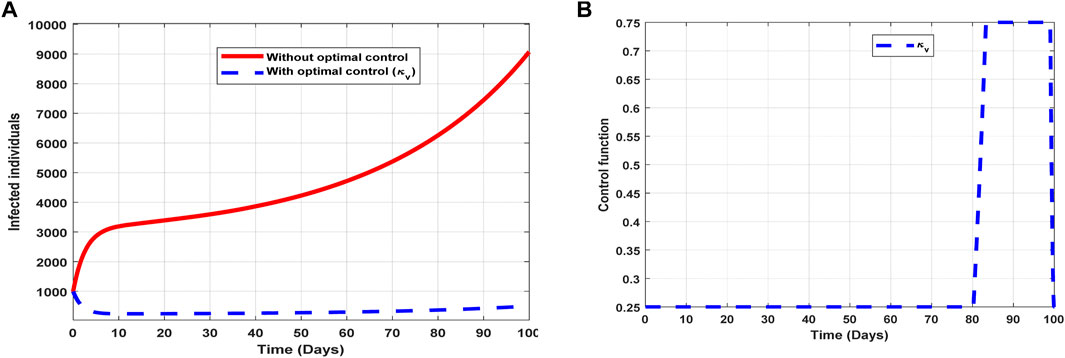
Figure 7. Optimal solutions of implementing strategy 2. Plot (A) blue dotted line is the optimal solution for implementing strategy 2. (B) Optimal control profile for strategy 2.
The optimal solutions illustrated above depict the following observations when vaccination is only applied:
(a) Figure 7A represents the effect of the control effort
(b) Figure 7B represents the profile of the control effort for vaccination to prevent COVID-19. It implies that approximately 25% of the population should be vaccinated within 80 days and intensified further up to 75% in the subsequent days throughout the implementation to halt COVID-19 transmission.
6.2.3 Strategy 3: implementation of infectivity treatment (
The optimal solutions illustrated in Figure 8 account for the observations when the control effort
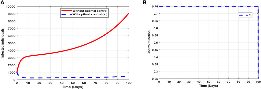
Figure 8. Optimal solutions of implementing strategy 3. Plot (A) blue dotted line is the optimal solution for implementing strategy 3. (B) Optimal control profile for strategy 3.
The optimal solutions illustrated above depict the following observations when infectivity treatment is only applied:
(a) Figure 8A represents the effect of the control effort
(b) Figure 8B represents the profile of the control effort for COVID-19 reinfection. It implies that approximately 75% of the individuals suspected to be carriers of the virus should be treated/monitored throughout the implementation to halt COVID-19 transmission.
6.2.4 Strategy 4: implementation of public awareness and vaccination (
The optimal solutions illustrated in Figure 9 account for the observations when the control efforts

Figure 9. Optimal solutions of implementing strategy 4. Plot (A) blue dotted line is the optimal solution for implementing strategy 4. (B) Optimal control profile for strategy 4.
The optimal solutions illustrated above depict the following observations when control efforts for public awareness and vaccination are applied:
(a) Figure 9A represents the effect of the control efforts
(b) Figure 9B represents the profile of the control efforts for public awareness and vaccination against COVID-19. It implies that approximately 80% of the population should be educated on COVID-19 within 22 days, which can be relaxed to approximately 25%, and 50% of the population should be vaccinated throughout the implementation of these interventions to halt COVID-19 transmission.
6.2.5 Strategy 5: implementation of public awareness and infectivity treatment (
The optimal solutions illustrated in Figure 10 account for the observations when all the control efforts
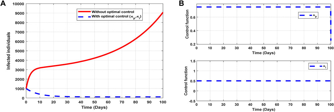
Figure 10. Optimal solutions of implementing strategy 5. Plot (A) blue dotted line is the optimal solution for implementing strategy 5. (B) Optimal control profiles for strategy 5.
The optimal solutions illustrated above depict the following observations when all the control efforts for public awareness and infectivity treatment are applied:
(a) Figure 10A represents the effect of the control efforts
(b) Figure 10B represents the profile of the control efforts for public awareness and infectivity treatment. It implies that approximately 80% of the population should be educated on COVID-19, and 50% of suspected carriers of the virus should be treated/monitored throughout the implementation of these interventions to halt COVID-19 transmission.
6.2.6 Strategy 6: implementation of vaccination and infectivity treatment (
The optimal solutions illustrated in Figure 11 account for the observations when the control efforts
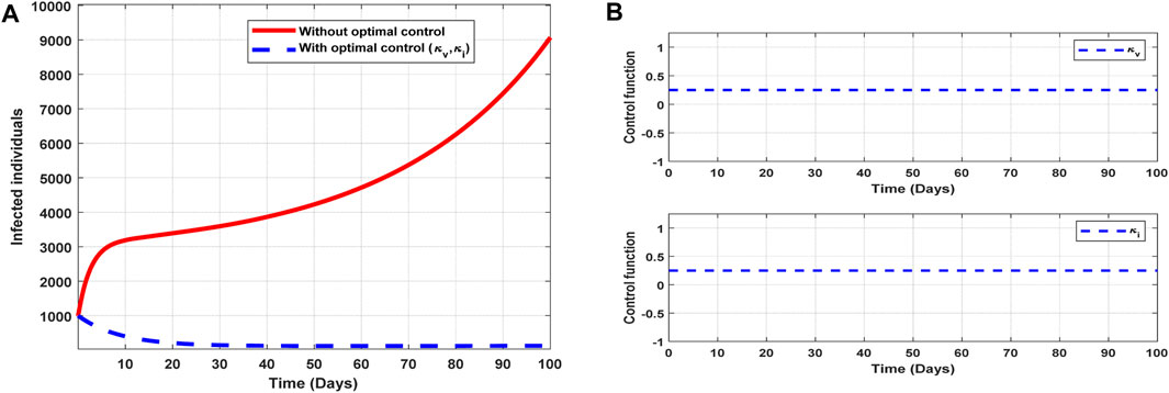
Figure 11. Optimal solutions of implementing strategy 6. Plot (A) blue dotted line is the optimal solution for implementing strategy 6. (B) Optimal control profiles for strategy 6.
The optimal solutions illustrated above depict the following observations when all the control efforts for vaccination infectivity reduction are applied:
(a) Figure 11A represents the effect of the control efforts
(b) Figure 11B represents the profile of the control efforts for public education and vaccination against COVID-19. It implies that all the interventions
6.2.7 Strategy 7: implementation of all controls (
The optimal solutions illustrated in Figure 12 account for the observations when the control efforts

Figure 12. Optimal solutions of implementing strategy 7. Plot (A) blue dotted line is the optimal solution for implementing strategy 7. (B) Optimal control profiles for strategy 7.
The optimal solutions illustrated above depict the following observations when all the control efforts are applied:
(a) Figure 12A represents the effect of the control efforts
(b) Figure 12B represents the profile of all control efforts. It implies that approximately 80% of the population should be educated on COVID-19, approximately 50% of the population should be vaccinated, and 50% of suspected carriers of the virus should also be treated/monitored throughout the implementation period of these interventions to halt COVID-19 transmission.
6.3 Cost–benefit analysis
Once the strategies are given, it is imperative to know the cost associated with implementing such intervention(s). Therefore, we explore the cost associated with each control strategy to check their effectiveness. We outline some cost-effectiveness approaches to further understand the control strategies.
We consider two procedures, namely, average cost-effectiveness ratio (ACER) and incremental cost-effectiveness ratio (ICER), which have been explained in [20–23], to carry out epidemiological studies.
6.4 Average cost-effectiveness ratio
We define the ACER of implementing a strategy as
The overall cost
From Table 4, control strategy 1, which involves the implementation of public education only, has the least value of ACER, indicating cost savings. However, relying solely on this metric is not enough to choose a strategy; hence, we further explore other approaches.
6.5 Incremental cost-effectiveness ratio
We define the ICER of implementing a strategy as
The total cost function
The ICER in Table 5 is calculated as
Assessing strategies 2 and 1 in Table 5, it is noticed from the ICER that strategy 2 is expensive to deploy in a resource-limited setting; therefore, strategy 2 is removed from the list of possible controls, and the ICER is calculated again. This is presented in Table 6.
Assessing strategies 1 and 4 in Table 6, it is noticed from the ICER that strategy 4 is expensive to deploy in a resource-limited setting; therefore, strategy 4 is removed from the list of possible controls, and the ICER is calculated again. This is presented in Table 7.
Assessing strategies 1 and 3 in Table 7, it is noticed from the ICER that strategy 3 is expensive to deploy in a resource-limited setting; therefore, strategy 3 is removed from the list of possible controls, and the ICER is calculated again. This is presented in Table 8.
Assessing strategies 1 and 5 in Table 8, it is noticed from the ICER that strategy 5 is expensive to deploy in a resource-limited setting; therefore, strategy 5 is removed from the list of possible controls, and the ICER is calculated again. This is presented in Table 9.
Assessing strategies 1 and 6 in Table 9, it is noticed from the ICER that strategy 6 is expensive to deploy in a resource-limited setting; therefore, strategy 6 is removed from the list of possible controls, and the ICER is calculated again. This is presented in Table 10.
Finally, assessing strategies 1 and 7 in Table 10, it is noticed from the ICER that strategy 7 is expensive to deploy in a resource-limited setting; therefore, strategy 7 is removed from the list of possible controls. Therefore, we conclude that strategy 1 is the most cost-effective strategy to use among the several strategies under study here. From the above analysis, it is obvious that strategy 1, which involves public education, is the intervention that saves cost.
7 Conclusion
We have presented a work that analyzes the changing effects of vaccination and infectivity reductions on the transmission of COVID-19 using data from Ghana. We have estimated the model’s parameters and analyzed their effects on disease transmission through numerical and graphical illustrations. Again, we have exhibited the threshold dynamics of the effective reproduction number
The aim of this work is to study the effect of vaccination and infectivity reductions in controlling COVID-19 transmission and devise control interventions that save cost to mitigate the transmission; therefore, we have formulated optimal control strategies together with the cost–benefit analysis that consider control measures involving both pharmaceutical and non-pharmaceutical interventions to control COVID-19. We implemented the strategies (Figure 6A–Figure 12A), and it was realized that public education, vaccination, and infectivity reductions to prevent COVID-19 should be intensified and reach approximately 25% of the population from the beginning and intensified in the subsequent days (Figure 6B–Figure 12B).
It is also worth knowing that public education saves cost as per the cost–benefit analysis compared to the other strategies raised in this work. This intervention can minimize COVID-19, as illustrated in Figure 6A. This intervention should reach approximately 50% of the population throughout the period of its implementation in order to realize the results of strategy 1 (Figure 6). Although strategy 1 saves cost, other strategies elaborated in this work can also be applied, but one has to consider the cost involved in implementing the strategy. The cost involved in applying the optimal control strategies is presented in Table 4–Table 10.
The outcomes of the findings imply that both pharmaceutical and non-pharmaceutical measures are very important in controlling the transmission of COVID-19. These control measures should always be vigorously implemented to create public awareness on COVID-19 and its reinfection, as illustrated in Figure 6B–Figure 12B, in order to reduce the effective contact rates and rates of acquiring COVID-19, as illustrated in Figure 3.
Although we have demonstrated the dynamics of COVID-19 transmission with vaccination and different infectivity reductions, this work is focused on the homogeneity of the population, and we hope to extend this study to explore the transmission dynamics of COVID-19 reinfection by considering heterogeneity of the population such as age and sex. We encourage individuals to adhere to personal hygiene and be aware of COVID-19 reinfection.
Data availability statement
The original contributions presented in the study are included in the article/Supplementary Material; further inquiries can be directed to the corresponding authors.
Author contributions
RA: conceptualization, data curation, formal analysis, investigation, methodology, writing–original draft, and writing–review and editing. ZJ: funding acquisition, supervision, and writing–review and editing. JY: formal analysis, supervision, and writing–review and editing. JA: formal analysis, investigation, and writing–review and editing.
Funding
The author(s) declare that financial support was received for the research, authorship, and/or publication of this article. This research was supported by the National Natural Science Foundation of China grants 12231012 and 61873154.
Acknowledgments
The authors appreciate the support of Complex Systems Research Center, Shanxi University.
Conflict of interest
The authors declare that the research was conducted in the absence of any commercial or financial relationships that could be construed as a potential conflict of interest.
Publisher’s note
All claims expressed in this article are solely those of the authors and do not necessarily represent those of their affiliated organizations, or those of the publisher, the editors, and the reviewers. Any product that may be evaluated in this article, or claim that may be made by its manufacturer, is not guaranteed or endorsed by the publisher.
References
1. World Health Organization. Coronavirus disease 2019(COVID-19), situation report -51, data as reported by 8 March 2020 (2019). Available at: https://www.who.int/emergencies/disease/novel-coronavirus-2019/situation-reports (Accessed January 10, 2024).
2. Chen Y, Wang Y, Fleming J, Yu Y, Gu Y, Liu C, et al. Active or latent tuberculosis increases susceptibility to COVID-19 and disease severity (2020). Available at: https://www.medrxiv.org/ (Accessed January 10, 2024).
3. Salman AM, Ahmed I, Mohd MH, Jamiluddin MS, Dheyab MA. Scenario analysis of COVID-19 transmission dynamics in Malaysia with the possibility of reinfection and limited medical resources scenarios. Comput Biol Med (2021) 133:104372. doi:10.1016/j.compbiomed.2021.104372
4. Zamir M, Nadeem F, Alqudah MA, Abdeljawad T. Future implications of COVID-19 through Mathematical modeling. Results Phys (2022) 33:105097. doi:10.1016/j.rinp.2021.105097
5. Worldometers. Reported cases and deaths by country or territory (2022). Available at: https://www.worldometers.info/coronavirus/#countries (Accessed April 30, 2022).
6. Zegarra MAA, Infante SD, Carrasco DB, Liceaga DO. COVID-19 optimal vaccination policies: a modeling study on efficacy, natural and vaccine-induced immunity responses. Math Biosci (2021) 337:108614. doi:10.1016/j.mbs.2021.108614
7. Adachi A. Grand challenge in human/animal virology: unseen, smallest replicative entities shape thewholeglobe. FrontMicrobiol (2019) 11:431. doi:10.3389/fmicb.2020.00431
8. 1mg. Coronavirus No-panic help guide (2020). Available at: https://smef.org.uk/wpcontent/uploads/2020/03/Corona-Ebook.pdf. (Accessed January 10, 2024)
9. Annas S, Pratama MI, Rifandi M, Sanusi W, Side S, Stability analysis and numerical simulation of SEIR model for pandemic COVID-19 spread in Indonesia. Chaos, Solitons and Fractal (2020) 139:110072. doi:10.1016/j.chaos.2020.110072
10. Pang L, Liu S, Zhang X, Tian T, Zhao Z, Transmission dynamics and control strategies of COVID-19 in Wuhan, China. J Biol Syst (2020) 28:543–60. doi:10.1142/s0218339020500096
11. Asamoah JKK, Owusu MA, Jin Z, Oduro F, Abidemi A, Gyasi EO, Global stability and cost-effectiveness analysis of COVID-19 considering the impact of the environment: using data from Ghana. Chaos, Solitons and Fractals (2020) 140:110103. doi:10.1016/j.chaos.2020.110103
12. Tchoumi S, Diagne M, Rwezaura H, Tchuenche J, Malaria and COVID-19 co-dynamics: a mathematical model and optimal control. Appl Math Model (2021) 99:294–327. e327. doi:10.1016/j.apm.2021.06.016
13. Yan X, Zou Y, Optimal and sub-optimal quarantine and isolation control in SARS epidemics. Math Comp Model (2008) 47(1-2):235–45. doi:10.1016/j.mcm.2007.04.003
14. Khan MA, Atangana A, Mathematical modeling and analysis of COVID-19: a study of new variant omicron. Physica A: Stat Mech Its Appl (2022) 599:127452. Article 127452. doi:10.1016/j.physa.2022.127452
15. Rwezaura H, Diagne M, Omame A, de Espindola A, Tchuenche J, Mathematical modeling and optimal control of SARS-CoV-2 and tuberculosis co-infection: a case study of Indonesia. Model Earth Syst Environ (2022) 8(4):5493–520. e5520. doi:10.1007/s40808-022-01430-6
16. Omame A, Abbas M, Onyenegecha C, A fractional-order model for COVID-19 and tuberculosis co-infection using Atangana–Baleanu derivative. Chaos, Solitons and Fractals (2021) 153:111486. Article 111486. doi:10.1016/j.chaos.2021.111486
17. World Health Organization. World health organization covid– 19 report (2024). Available at: https://covid19.who.int/region/afro/country/gh. (Accessed January 10, 2024).
18. Dietz K. The estimation of the basic reproduction number for infectious diseases. Stat Methods Med Res (1993) 2:23–41. doi:10.1177/096228029300200103
19. Osei E, Amu H, Kye-Duodu G, Kwabla MP, Danso E, Binka FN, et al. Impact of COVID-19 pandemic on Tuberculosis and HIV services in Ghana: an interrupted time series analysis. PLoS ONE (2023) 18(9):e0291808. doi:10.1371/journal.pone.0291808
20. Asamoah JKK, Owusu MA, Jin Z, Oduro FT, Abidemi A, Gyasi EO, Global stability and cost-effectiveness analysis of COVID-19 considering the impact of the environment: using data from Ghana. Chaos, Solitons and Fractals (2020) 140:110103. doi:10.1016/j.chaos.2020.110103
21. Agusto F, Leite M, Optimal control and cost-effective analysis of the 2017 meningitis outbreak in Nigeria. Infect Dis Model (2017) 4(2019):161–87. doi:10.1016/j.idm.2019.05.003
22. Asamoah JKK, Okyere E, Abidemi A, Moore SE, Sun G, Jin Z, et al. Optimal control and comprehensive cost-effectiveness analysis for COVID-19. Results Phys (2022) 33:105177. doi:10.1016/j.rinp.2022.105177
Keywords: COVID-19, vaccination, infectivity reductions, optimal control, cost–benefit analysis
Citation: Appiah RF, Jin Z, Yang J and Asamoah JKK (2024) Cost–benefit analysis of the COVID-19 vaccination model incorporating different infectivity reductions. Front. Phys. 12:1383357. doi: 10.3389/fphy.2024.1383357
Received: 07 February 2024; Accepted: 19 March 2024;
Published: 08 May 2024.
Edited by:
Xiaoke Xu, Dalian Nationalities University, ChinaReviewed by:
Xiaofeng Luo, North University of China, ChinaSegun Oke, Ohio University, United States
Copyright © 2024 Appiah, Jin, Yang and Asamoah. This is an open-access article distributed under the terms of the Creative Commons Attribution License (CC BY). The use, distribution or reproduction in other forums is permitted, provided the original author(s) and the copyright owner(s) are credited and that the original publication in this journal is cited, in accordance with accepted academic practice. No use, distribution or reproduction is permitted which does not comply with these terms.
*Correspondence: Zhen Jin, amluemhuQDI2My5uZXQ=; Junyuan Yang, eWp5YW5nNjZAc3h1LmVkdS5jbg==
 Raymond Fosu Appiah
 Zhen Jin
 Junyuan Yang
 Joshua Kiddy K. Asamoah