
94% of researchers rate our articles as excellent or good
Learn more about the work of our research integrity team to safeguard the quality of each article we publish.
Find out more
REVIEW article
Front. Phys. , 10 June 2024
Sec. Optics and Photonics
Volume 12 - 2024 | https://doi.org/10.3389/fphy.2024.1383256
 O. V. Angelsky1,2
 A. Y. Bekshaev3
 P. P. Maksimyak2
 I. I. Mokhun1
 C. Y. Zenkova1,2
 V. Y. Gotsulskiy3
 D. I. Ivanskyi2
 Jun Zheng1*
The review describes the principles and examples of practical realization of diagnostic approaches based on the coherence theory, optical singularities and interference techniques. The presentation is based on the unified correlation-optics and coherence-theory concepts. The applications of general principles are demonstrated by several examples including the study of inhomogeneities and fluctuations in water solutions and methods for sensitive diagnostics of random phase objects (e.g., rough surfaces). The specific manifestations of the correlation-optics paradigms are illustrated in applications to non-monochromatic fields structured both in space and time. For such fields, the transient patterns of the internal energy flows (Poynting vector distribution) and transient states of polarization are described. The single-shot spectral interference is analyzed as a version of the correlation-optics approach adapted to ultra-short light pulses. As a characteristic example of such pulses, uniting the spatio-temporal and singular properties, the spatio-temporal optical vortices are considered in detail; their properties, methods of generation, diagnostics, and possible applications are exposed and characterized. Prospects of further research and applications are discussed.
Electromagnetic fields are ubiquitous in Nature, and almost any process occurring in the material World is associated with a sort of generation, radiation, absorption or transformation of various electromagnetic waves. This stipulates the exceptional role of electromagnetic fields as unique witnesses carrying information about the most important physical phenomena, from the Big Bang and expansion of the Universe to the lepton and hadron interactions on sub-nuclear scales. In all such processes, electromagnetic fields are involved; they differ mainly by the characteristic wavelengths λ but the principles governing their physical behavior are universal.
The waves of optical range that expands from sub-millimeter to nanometer scales (λ ∼ 10−4 ÷ 10−8 m) are compatible with the most common atomic, molecular and structural processes occurring in various sorts of physical matter. That is why it is the optical methods that are especially suitable for testing, diagnostics and investigation of diverse physical systems, as well as for their purposeful transformations and manipulations. Such optical methods demonstrate a remarkable progress in the past years, stipulated by the development of new optical technologies based on the enhanced opportunities of light structuralization which involves not only spatial but also temporal and spectral dimensions [1–5]. The new possibilities for the light-field formation and characterization essentially enhanced the technical power in the optical means for study and control of matter but also have changed some common-sense optical paradigms. Now, it is not surprising that optical energy can be concentrated and fruitfully manipulated in the volumes, orders of magnitude smaller than the wavelength, and controllably released with the attosecond temporal resolution [6]. Simultaneously, the powerful theoretical instruments, involving the stochastic and correlation description of light fields [7–13] preserve their value and heuristic abilities.
In this paper, we make an attempt of describing some modern optical-diagnostic possibilities, based on the traditional correlation optics, coherence theory and interference technique. This ground enables us to consider, from the unified initial positions, different problems of optical diagnostics. After the short introduction into the optical coherence theory (Section 2), applications of its principles are demonstrated in the study of physical inhomogeneities and fluctuations in liquid media, especially, in water solutions (Section 3.1). The interference technique for sensitive detection of the solutions’ optical constants is discussed, as well as the approach of laser correlation spectroscopy for analysis of non-stationary perturbations in the sample. In Section 3.2, the methods for sensitive diagnostics of random phase objects, e.g., rough surfaces, are exposed and discussed.
In Section 4, the correlation-optics principles are refined and further adapted for optical fields with essential temporal structuring, e.g., non-monochromatic fields. The specific transient patterns of the light energy distribution, non-stationary polarization states, and the internal energy flows are discussed, with the special attention to their singularities and possible manifestations in the observable (time-averaged) field behavior. This way naturally brings the presentation to the topic of spatio-temporal light fields which are characterized by the non-separable structure variations in the space and time (spectral) coordinates (Section 5). As an example of such fields, the spatio-temporal optical vortices are considered in more detail as optical objects in which the high degree of 4D structuralization is combined with the essential singular nature. These features make them exemplary objects of highly developed and topologically organized wave packets. Their unique properties, methods of investigation, generation, and possible applications are described and characterized. Traditionally, the review is finished by Conclusion presenting a summary of the results achieved and some prospects of further activity in research and applications.
Modern approaches for quantitative characterization of light fields with arbitrary degree of coherence, structured both in time and space, start with the Wolf’s introduction of the field’s statistical correlation moments [7–13]. The matter is that the underlying field parameters (instantaneous electric and magnetic vectors) are not observable but the field is characterized by their spatial and temporal (and, possibly, mixed spatio-temporal) correlation moments. This paradigm enables to quantitatively describe the optical-field state, its transformations and evolution in a unified physically consistent manner compatible with usual conditions of optical experiments and applications. On this base, multiple methods for metrological assessment of the light field’s characteristics including the distributions of amplitude, phase, polarization, etc., have been developed, and novel approaches, with additional capacities and metrological power, regularly appear. In these methods, the possibilities of studying the field structure in linear (first-order moments), quadrature (second-order moments) and higher approximations (involving the higher-order statistical moments of the underlying field characteristics) are realized [7–13].
The basic instrument of the correlation optics is the cross-coherence function defined as [7, 12].
where
where
Temporal behavior of the fields is closely related to their spectral inhomogeneity [11–13]. Accordingly, the correlation properties of the field can be characterized by the cross spectral density which is defined via the Fourier transform of the cross-correlation function (1):
Generally, the cross spectral density can be expressed through the single-point spectral density
and the spectral degree of coherence
The spectral density (4) determines the correlation properties of the field in the same point R, whereas the spectral degree of coherence
Quantities 1-5 supply an exhaustive statistical characterization of scalar optical fields whose polarization is homogeneous and linear. But most of optical phenomena essentially involve the vector nature of light waves, and their statistical characterization requires to consider the vector stochastic processes which can be analyzed based on the Maxwell theory [14]. In general, the different orthogonal polarization components behave independently, and their mutual correlations can be considered in the frame of the coherence matrix [9, 10, 14–20] which is an immediate generalization of the scalar cross-correlation function 1. For paraxial fields mainly characterized by the transverse electric-field components Ex, Ey, the coherence matrix obtains the general form
where
where Det and Tr denote the matrix determinant and trace, correspondingly.
The relations (6), (7) and their derivatives, as well as the concepts these involve, form a basis for fruitful studies of the vector optical fields and their metrological applications in many applied and fundamental problems [18–21]. Coherence matrices, combining the coherence and polarization features of optical fields, constitute the ground for a powerful methodological approach to describing the optical-fields characteristics and their variations induced by light-matter interactions.
The general framework schematically outlined in Section 2 can be employed for multiple applied problems. In this context, it is especially interesting to consider the potential capabilities of the optical metrology methods for parametric characterization of some well-known systems, which have been traditional objects of comprehensive studies for a long time. On the one hand, this activity offers good opportunities for the methods’ evaluation and testing; on the other hand, it shows the aspects that require additional in-depth research and analysis of future prospects. In this Section, we illustrate the main characteristics, capacities and prospects of the interference approach, based on the typical examples stemmed from the authors’ experience.
In this context, we consider several demonstrative situations illustrating the power of the correlation-interferometry technique. The first one concerns the problem of high-precision measurement of the refractive-index variations in optically transparent aqueous solutions [22, 23]. Such measurements are highly important because the nature of the molecular interaction in a liquid determines the polarizability of molecules, and hence the refractive index. Consequently, the changes of polarizability, that accompany changes in the physical state of a solution, can be used to assess the short- and long-range molecular interactions. The long-range molecular interactions in a liquid manifest themselves in the form of a quasi-crystalline structure of water, similar to the structure of ice [22, 23]. For such media, the refractive index is related with the medium permittivity ε and can be described by relation [24]
where θ is the polarizability-correlation parameter, N is the concentration of particles (molecules of water and/or solved substance), and α is the polarizability of a single particle. According to Eq. 8, knowledge of the refractive index distribution gives a possibility to estimate spatial variations of the parameters θ, N and α which characterize fine processes of the molecular interactions and structure formation.
In the scheme of [22, 23], a Mach—Zehnder or Michelson interferometer is used, formed by the elements 3, 5, and 7 (Figure 1). The CW radiation generated by laser 1 passes the collimator 2 whence the quasi-plane-wave beam enters the beam splitter, and the two linearly-polarized beams with equal intensities are formed. One of these beams passes through the water-medium sample 4; the reference beam is obtained by reflection from mirror 7, and its polarization is set orthogonal by the quarter-wave plate 6. At the interferometer exit (branch 3–14), the beams are arranged strictly coaxial, and their polarizations are transformed into orthogonal circularly polarized states by means of the quarter-wave plate 10. Their interference results in a linearly polarized beam with the polarization direction depending on the phase retardation of the signal beam, i.e., on the refractive index of the investigated sample 4. Accordingly, any changes in the refractive index (8) caused by any external or internal impact (temperature, chemical transformations, mechanical disturbances) are manifested in a change of the linear-polarization azimuth at the interferometer output, which can be detected, e.g., by the analyzer 11. Modern modulation systems for the polarization measurements enable to evaluate the change in the linear-polarization azimuth at the level of one arc second. This, in turn, makes it possible to measure changes in the wave-path difference between the interferometer arms at a level of 0.5–1 nm [22, 23].
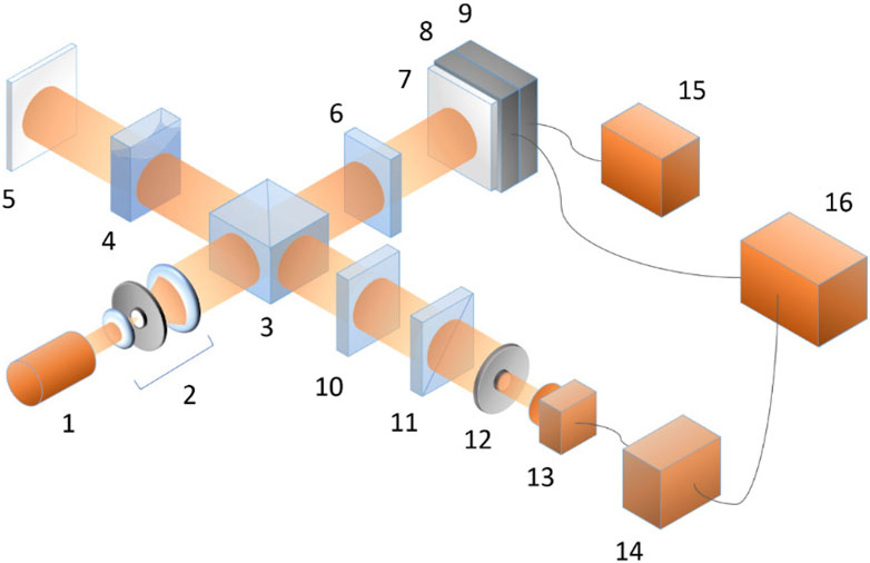
Figure 1. Experimental arrangement for measurement of the refractive-index variations in aqueous solutions: (1) single-mode laser; (2) collimator; (3) beam splitter; (4) liquid sample; (5, 7) mirrors; (6, 10) quarter-wave plates; (8, 9) piezoceramic modulators; (11) analyzer; (12) field diaphragm; (13) photodetector; (14), phase-sensitive electronic amplifier; (15) power supply; (16) recorder.
Therefore, at the same level of accuracy one can measure variations in the refractive index of the solution, and thus judge on the underlying microscopic phenomena [25–27]. This means that optical interference instruments, involving the principles of heterodyning, enable to study the intra-atomic and intra-molecular processes in optically transparent, weakly absorbing aqueous media.
In the above-described example, the interference technique was applied to spatially homogeneous fields with the phase difference being the only determinable parameter. This situation can be treated as an interference pattern with the single fringe of infinite width. However, the interference approaches can be equally useful for optical diagnostics of spatially inhomogeneous fields where the phase difference between the compared beams depends on transverse coordinates. The corresponding techniques can be applied for investigation of the influence of fluid mechanical disturbance (dynamics) on the spatial and/or temporal variations of the refractive index. To date, these processes have been studied insufficiently; only small steps have been taken in this direction. In particular, Ref. [27] presents the results related to anomalous light scattering [28, 29] in water-glycerol solutions that were prepared by diffusion in a gravitational field. This made it possible to cover the entire concentration range of existence of solutions in a single sample. The spatial distribution of the solution concentrations was obtained by the modification of the interference method known as the electronic speckle-pattern interferometry (ESPI) [30, 31].
Among various approaches to optical diagnostics of the condensed states of matter, especially liquids, one of the most efficient is the method of laser correlation spectroscopy (LCS) [32, 33]. Its first applications in the middle of the 20th century were associated with astrophysics at the intersection of optics and radio-physics. But with the appearance of lasers in physical laboratories, it quickly became popular for determining the properties of dispersed systems, liquid crystals, biological molecules, as well as spatial inhomogeneities and matter flows of various scales [34–36]. Because this technique is based on the scattering of light by moving objects, it is sometimes referred to as “dynamic light scattering” (DLS). However, the DLS is a broader category and includes a number of other methods based on the interaction of highly coherent radiation with moving objects, for example, laser Doppler anemometry [35].
In most works, the LCS principles are interpreted based on the radio-physical approach, where fluctuations of the scattered-light intensity δI are described as beatings that arise as a result of the interference of waves with frequencies shifted due to the Doppler effect. Within the framework of classical spectroscopy, when light is scattered by a system of moving objects, the monochromatic probe-radiation spectral line broadens by the Doppler-shifted sidebands. However, the characteristic spectral-line broadening in various problems is about
According to Eqs 3, 4,
The principles of LCS can be easily understood using the example of the frequently employed experimental arrangement of optical homodyning (Figure 2). Here, highly coherent probing radiation is scattered by optical inhomogeneities of the object, which performs random phase modulations. The size of the observed scattering volume is limited by the aperture d1. The scattered wave possesses a characteristic speckle structure [30, 31], and the second aperture diaphragm d2 separates a small portion of scattered light propagating at an angle θ. Since scattering occurs in the object with movable optical inhomogeneities, the speckle pattern is variable, and its changes in time are determined by the arrangement parameters and by the nature of the motions in the object of study. In order to record the temporal intensity variations, the diaphragm d2 should select no more than one speckle. Therefore, the geometry of the experiment must satisfy the relation
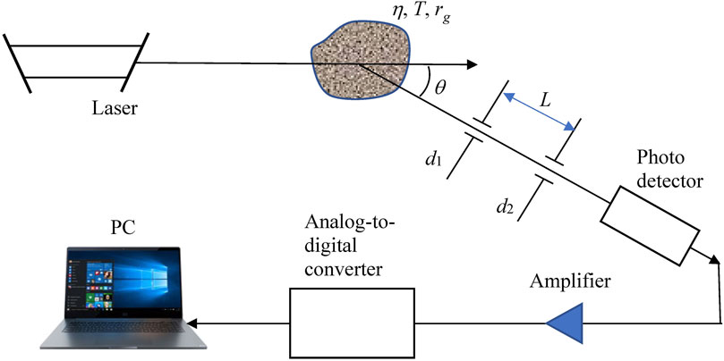
Figure 2. Homodyning scheme for the LCS (explanations in text).
Remarkably, in this method, the scattered light is observed immediately, without intermediate confrontation to the delayed or shifted probing-beam copy, immanent in the interference schemes (see, e.g., Section 3.1). This circumstance is favorable for simplicity and controllability of the equipment but puts additional requirements to the probing-radiation stability and spectral purity. In the scheme of Figure 2, the photodetector behind the diaphragm
and, for more complex situations
with properly adjusted parameters a, b, C.
The second problem is associated with the very low intensities of scattered light. Therefore, photomultipliers in the photon-counting mode have traditionally been used as photodetectors, which in modern devices are replaced by the avalanche diodes. Then, the photo-counts can be recorded with a rather simple optical equipment, after which the entire data stream is easily converted into digital format, and the further signal processing and storage of both the original data and the results of their processing depend only on the power of the digital part of the device and software solutions. In particular, the correlation function of intensity can be found via accumulation of photo-counts registered for several consecutive pulses [37, 38].
Normally, in the LCS method, the light scattered by Brownian particles is more intense and therefore more conveniently registered than the signal formed directly by the medium fluctuations. For this reason, the particles can be used as sensitive microscopic probes providing access to specific details of the molecular processes in liquid. For example, when studying the cluster structure of water-ethanol solutions in the vicinity of their singular point (the isotemperature point of contraction at 0.08 mol fraction of alcohol), latex particles were used in such low concentrations that they did not change the solution properties [39, 40]. It was found that at alcohol concentrations lower and higher than the singular point, the specific features in the particles’ mobility exist, which confirmed the emergence of micro-inhomogeneous structures of such solutions with different types of ordering.
In application to liquid and aqueous media, the interference techniques, briefly outlined in this Section, can be used for detection and characterization of specific topological wave structures whose existence in such systems has been recently demonstrated: phase vortices, skyrmions, merons, etc. [41–43]. These structures are well known in quantum physics and classical optics but the gravity and capillary surface waves in liquids offer very demonstrative and easily attainable realization of their principles illustrating the universal topological phenomena associated with wave fields. These topological structures naturally appear during interference of linear surface waves in water and can be efficiently controlled via regulation of the amplitudes, phases, frequencies (spectral composition) of the interfering waves, i.e., the same set of instruments that is used for optical fields in the correlation-optics framework. Their observation can be realized in the arrangements similar to those of Figures 1, 2 with the spatially-resolving detection of local phase differences via the spatially inhomogeneous interference patterns [21]. Additionally, their specific dynamical features may be favorable for implementation of the dynamical influence on the optical characteristics of liquids, in particular, on their refractive index (discussed in Section 3.1.1).
As a general inference of the above presentation, one may note that, currently, the idea of metrological assessment of the statistical consistency, both in time and in space, for wave fields has been practically implemented. Flexible, reliable and attainable interference approaches for metrological evaluation of the field correlation moments (including the mixed moments, describing, e.g., correlations between the amplitudes and phases of the fields involved) of different orders have been developed [44].
The ideology underlying the design and composition of such metrological systems is based on the concept of phase object (PO). From now on, the term “PO” means a material object whose influence on the input radiation can be reduced to the phase modulation of the output (reflected or transmitted) beam; of course, this “pure” phase modulation can only be observed immediately after the light-object interaction, i.e., in the “boundary zone” [44, 45] (with further propagation, the phase modulations inevitably induce the amplitude inhomogeneities). In many cases the PO-induced phase transformations are random and are directly associated with the irregularities of the object transmission or reflection coefficients, which can be described in a unified way as
where the input field amplitude
Since the information about a random PO is obtained from the optical radiation interacting with it, the random PO diagnostics must be carried out in two stages. The first one is identifying the relationships between the object statistical properties and the probe-field correlation parameters for different recording zones; the second one is the practical measurement of the probe field correlation parameters of necessary orders and with appropriate accuracy [47].
The problem is usually considered using a model of infinitely extended random POs. It is based on the approaches proposed, tested and implemented within the framework of statistical radio-physics [44]. Its main assumptions are: 1) all spatial-frequency components corresponding to the PO phase structure contribute to formation of the radiation field resulting from the light-object interaction; 2) the dispersion
The diagnostics of the PO structure is relatively simple if the random phase modulations obey Gaussian statistics. In this case, a complete description of the object is supplied by its mean phase and phase dispersion [54]. There is a unique and direct relationship between the phase dispersion of an object and the relative contrast of the speckle field obtained due to its interaction with the probing optical field [54]. By measuring the speckle-field contrast in different recording zones, one can obtain the object phase dispersion
Within the framework of this formulation of the diagnostic problem [48, 50], the unambiguous relation was found between the transverse coherence function
where
For objects with
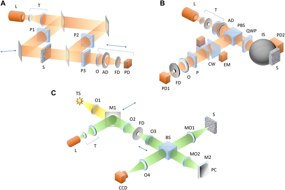
Figure 3. (A) Schematic view of the setup for measuring the correlation moments of the random PO [48]; (B) Optical arrangement for surface roughness measurements with sub-wavelength transverse size of inhomogeneities; (C) Experimental arrangement for PO diagnostics with large longitudinal inhomogeneities. Notations: (L) laser; (TS) temporal source; (T) telescopic system; (S) sample; (P, P1, P2, P3) polarizers, (O, O1, O2, O3, O4) objectives; (MO1, MO2) micro-objectives; (AD) aperture diaphragm; (FD) field diaphragm; (BS) beam-splitter; (PBS) polarizing beam-splitter; (QWP) quarter-wave plate; (IS) integrating sphere; (CW) calcite wedges; (EM) electromechanical modulator; (M1) movable mirror; (M2) mirror; (PC) piezo-ceramics; (PD, PD1, PD2) photodetectors; (CCD) camera.
In this scheme, a quasi-plane-wave beam is formed by the laser source L and the collimator T, after which it is divided into the object arm (elements P1, S) and the reference arm (element P2). The object-arm beam impinges the sample S perpendicular to its surface (in Figure 3A, the transparent sample of fused quartz is implied but simple modifications of the same scheme enable testing the reflecting surfaces). The resulting beam obtained after passing the sample is superimposed with the reference beam; the mixed output beams are collinear. The unwanted displacements of the compared beams in the longitudinal direction somewhat hamper measuring the object inhomogeneity. To avoid this difficulty, a method for measuring the phase dispersion was chosen, which connects the mixed third-order correlation moment of the amplitude fluctuations with the phase dispersion function. The imaging system, containing the objective O and diaphragms AD, FD, projects the resulting intensity distribution onto the photodetector PD input plane. The observed pattern expresses the interference between the plane reference wave and the phase-modulated object wave, which enables to find the relation between the phase dispersion and the normalized value of the intensity inside the averaging area [48]
Here
There is a connection between the field scintillation index and its phase dispersion, on the one hand, and a set of statistical moments that characterize the statistical structure of an object [44]. In particular, knowledge of the correlation moments of a random field up to the fourth order enables to approximate the characteristic function (spatial-frequency distribution) of this field θ(κ) [56]. In turn, the characteristic function determines the distribution function of the heights h of irregularities for the examined rough surface in the form
This way determines the distribution function with relative error not exceeding 5%–7% [56]; the available sensitivity of the roughness irregularity measurements reaches ∼5 Å [48, 54]. In a whole, the above results form a basis for the development of metrology methods for high-speed, high-precision device prototypes, which have been successfully verified in a series of consistent metrological tests.
Optical diagnostics of surfaces with a roughness transverse size comparable to λ require extracting the information that is contained in high-spatial-frequency components of the reflected (scattered) field. This problem can be solved with a modified approach in which the regular and diffuse parts of the reflected radiation are spatially separated [49, 50], and the surface roughness characteristics are evaluated from the interference measurement of the regular part and photometric measurement of the diffuse part of the object wave.
To this end, in the optical arrangement of Figure 3B [49], a single-mode He-Ne laser radiation (λ = 632.8 nm) is used, which forms a quasi-plane-wave beam after passing a telescopic system T. Then, a homogeneous component of the beam is separated by means of the diaphragm AD. Its polarization is directed according to the transmission plane of the polarizer cube PBS, making a 45° angle with the principal axis of the quarter-wave plate QWP. Afterwards, the beam enters the integrating sphere IS to interact with the surface of the tested sample S. The resulting beam intensity Ip is composed of three contributions: 1) coherent part Ic, which leaves the photometric sphere after being reflected from the surface, 2) stochastically reflected light Is propagating within the coherent beam aperture, and 3) diffusely reflected light Id which is “caught” by the photometric sphere. The beams Ic + Is pass through the quarter-wave plate QWP twice, thus experiencing a 90° rotation of the plane of polarization. Therefore, the beams Ic + Is undergo a total reflection from the beam-splitting face of the cube PBS and enter the displacement interferometer formed by two calcite wedges CW that implement a plane-parallel plate and a polarizer. The principal axes of the wedges coincide and make a 45° angle with the plane of polarization of the beam approaching from the cube PBS, while the polarizer P transmission plane makes a 90° angle with this plane. The image of the surface S is projected onto the field-diaphragm plane FD, after which it is registered by a photodetector PD1. The diffusely reflected beam intensity Id is measured by a power detector PD2. The transverse relative displacement of the beams mixed in the polarization interferometer, which is necessary for measuring the coherence function
The schemes and approaches outlined in the above paragraphs form the basis of efficient diagnostic systems for various surfaces, e.g., those assigned for applications in optical, semiconductor, and microelectronic techniques. These are especially valuable for the quality control of ultra-smooth, slightly rough surfaces, where the achieved sensitivity, estimated by the height parameter (the standard deviation of the rough surface profile from the baseline) is ∼3–5 Å, and the response speed is at the level of 1 s [50].
Further developments of the correlation-optics techniques, based on the random PO model, for the rough surface diagnostics, are coupled with their extension to objects with non-Gaussian statistics, fractal random surfaces, and coarse surfaces with the height variations exceeding the probing beam wavelength [21]. In such cases, the statistical properties of fractal surfaces can be most naturally described via the spatial power spectrum of the surface inhomogeneity h(x,y) rather than by the correlation function [50–52].
Relating the spatial structuring of light scattered by rough surfaces of different natures, interesting problems emerge in the framework of their distant diagnostics. Here, the two situations can be singled out and separately analyzed. The first one appears when the dispersion of the surface-inhomogeneity heights is comparable or exceeds the wavelength of the probing coherent beam, and there is no specular component of the reflected radiation. Accordingly, the unambiguous connection between the statistical parameters of roughness and scattered field is lost. To diagnose such surfaces, new approaches of fractal and singular optics are employed [51, 52]. However, such approaches only provide classification of rough surfaces, distinguishing the random and fractal ones.
In this case, the task of optical diagnostics requires an employment of additional means from the arsenal of correlation-optics tools. Namely, together with the usual transverse field correlations, it is necessary to study how the longitudinal coherence function of the incident beam is transformed, and to quantitatively assess this transformation. It is quite appropriate to assume that the longitudinal coherence function of the object field appears as a convolution of the longitudinal coherence function Γ0(∆z) of the probing beam and the distribution function F(h) of the heights of irregularities of the surface under study [53]:
where F(h) describes the statistical distribution of the partial signal delays determined by the surface inhomogeneities (cf. Eq. 11).
The experimental determination of the longitudinal coherence function is coupled with difficulties caused by the unequal visibility of the resulting interference pattern, which originate from the, generally, polychromatic nature of waves with finite coherence length lc. To overcome these difficulties, a Michelson interferometer was engaged (see Figure 3C), in which a monochromatic or polychromatic image of the rough surface (formed by elements MO1, O4 at the CCD input plane) is mixed with a monochromatic or polychromatic reference field formed by the mirror M2 [53, 54]. Herewith, it is admissible that the depth of phase modulations caused by the surface relief may exceed the coherence length of the probing radiation.
Nevertheless, the interference between the phase-modulated object beam and a coherent reference beam having a smooth simple-shape wavefront, supplies sufficient information for solution of the diagnostic problems [53, 54]. The 3D interference pattern depends on the local value z of the optical path difference between the beams:
where I0 is the reference wave intensity, Is (x,y) is the object-wave intensity distribution (the rough-surface image) in polychromatic light, and z0 is an arbitrary starting position, which is controllable by means of piezoceramics PC (Figure 3C). This example demonstrates that the data, obtained using partially-coherent (in time) probing radiation, supply an additional channel for information on the structure of rough surfaces with large inhomogeneities h > λ. The results can be obtained after the proper analysis of the interference fringes and are related to the last (cosine) multiplier of Eq. 13 responsible for the pattern visibility.
Another situation occurs in the opposite case of slightly rough (weakly structured) surfaces, where the phase inhomogeneities are distributed with dispersion much less than 1, and their transverse dimensions are significantly smaller than the wavelength. In this case, it seems that the most efficient and facilitative method is based on the use of micro- or nanoparticles that “feel” the surface-induced optical-field structure via optical forces that cause their concentration near special points (intensity minima, maxima, saddle points, etc., forming the field “skeleton” [1, 57–59]) and, in this manner, visualize the details of the surface relief. In this context, the specially designed carbon nanoparticles look especially useful as metrological probes [21, 47, 55, 60]. The latest results demonstrate the possibility of studying distant objects in real time by analyzing the skeleton of the scattered speckle field and studying the behavior of carbon nanoparticles under the influence of internal energy flows of this field. The carbon nanoparticles have been successfully used for reconstruction of the 3D landscape of super-smooth surfaces, with the lateral resolution ∼10 nm, fairly surpassing the well-known Abbe limitations of optical imaging systems [47, 55, 60].
Last examples of the previous Section have illustrated the useful utilitarian properties of probing beams with low temporal coherence, and thus lead us to understanding the special importance of non-monochromatic (although spatially coherent) light for optical-diagnostic problems. Such fields show certain specific statistical and dynamical features which are briefly discussed in this Section.
The concept of transient superposition was introduced for characterizing the phenomena obtainable with quasi-monochromatic beams of slightly different central frequencies [61]. Let us consider two waves for which the electric field values can be represented by Fourier integrals:
(from now on, symbols with tilde “∼” denote “true” instantaneous characteristics, in contrast to the time-averaged ones which will be in the focus of further analysis). Here R = (x, y, z)T denotes the spatial coordinates (superscript “T” means the matrix transposition), the spectral densities can be presented in the form
In turn, it is suitable to suppose the separability of the spatial and spectral arguments in
so the waves’ amplitudes are determined by
Additionally, to reflect the real situation of quasi-monochromatic waves, we suppose
where
We consider superposition of waves (14) that forms a resulting field
According to the classic theory of the second-order coherence [61], the waves
The most important results are associated with the last (interference) term of (19), I1,2. By using relations (15)–(18), its time-averaged value with sufficient accuracy can be described by equation
where
The quantity
and possess similar phase distributions such that
where the function
which supplies the usual expression of beatings observable in the superposition of waves with different frequencies. Eq. 23 describes the slowly-varying interference pattern moving with the velocity determined by the difference of the central frequencies.
The latter results of the previous Section testify that some essential features of the non-monochromatic optical fields can be understood via the simplified analysis of a bi-chromatic superposition containing only two frequencies (Eq. 22). In Section 4.1, the scalar field model was considered which is applicable to beams with a homogeneous linear polarization [58, 59]; now we address a bit more complex situation where the superposition includes two vector paraxial beams with arbitrary polarization in the transverse cross section.
In this case, it is suitable to start with the explicit expressions for bi-chromatic superposition that follow immediately from the vector analogs of Eqs. 14, 22:
where
(ex, ey, and ez are the unit vectors of a Cartesian frame). In turn, the complex amplitude components are characterized by their own amplitudes
For illustration, we consider the field behavior in a single point of the beam cross section, which allows one to omit the coordinate dependence of (26). Then, Eqs 24, 26 determine the instantaneous behavior the electric field components. It is suitable to choose the time-scale origin so that
These relations describe the instantaneous behavior of the electric field in a bi-chromatic polarized wave [62–66]. In contrast to the usual linear or elliptic polarizations, observed in monochromatic fields, here the electric vector describes rather complex trajectories. If the frequencies ω1 and ω2 are commensurate, the trajectories are similar to the Lissajous figures [67] repeatedly reproduced with the beating period
where ⟨…⟩ means the average over the beating period (“moments of inertia tensor” of the Lissajous figure [62, 63]). This matrix is similar to the real coherence matrix (6) at τ = 0 and to the moment matrix in parametric characterization of the beam transverse profile [20, 68]. The Lissajous singularities appear as the generalizations of the usual monochromatic polarization singularities [69, 70] in points where the eigenvalues of the matrix (28) are equal and where at least one of the eigenvalues vanishes (analogs, respectively, of the C-points and s-contours [69, 70]). Such structures naturally appear in the processes of higher-harmonic generation where N1 = 1, N2 = 2, 3, … [62–64], and the involved beams are spatially inhomogeneous.
Here, we briefly consider the instantaneous field in a single point; in this case, Eqs 27 allow to disclose the formation mechanism of the time-averaged characteristics in the general polychromatic case [71]. Some numerical results are presented in Figure 4, which illustrates the case of superposition of beams with orthogonal linear (circular) polarizations. This situation is free from the limitations associated with the harmonic generation, and the conditions N1 = 4, N2–N1 = 1 (ω2/ω1 = 1.25) are accepted. Accordingly, the electric-field-vector motion is periodic with the period depending of the frequency difference,
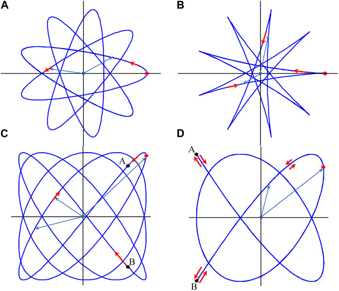
Figure 4. Trajectories described by the electric-field vector in the cross section z = 0 of the superposition (27) of (A, B) circularly polarized waves with a1,2y = a1,2x = a1,2, Δφ1 = π/2, Δφ2 = –π/2 and (C, D) linearly polarized waves with a1y = 0, a2x = 0, Δφ1 = Δφ2 = 0. In all cases the frequencies relate as ω2/ω1 = 1.25; the ratio of amplitudes a2/a1 is (A) 0.5, (B) 0.8 and (C, D) 1 (a2y = a1x); the initial phase difference φ21 is (A, B) 0; (C) 0.1π and (D) 0.25π. Thin gray arrows starting at the coordinate origin show some current electric vector positions, the red asterisk denotes its initial position at the moment t = 0, red arrows show the direction of its motion with time; in points A and B (black asterisks), handedness of the electric-vector rotation changes. The whole duration of the trajectory evolution equals to the beating period
Notably, in Figures 4A, B, the electric vector always rotates in the positive (counter-clockwise) direction while in Figures 4C, D, the rotation handedness changes inside the single period (in points A and B). This corresponds to the zero average handedness of the electric field rotation, which is an example of the Lissajous singularity [62, 63] analogous to that realized at points of s-contours in monochromatic fields [1, 59, 70]. The complicated electric-vector trajectories associated with arbitrary bi-chromatic and, generally, polychromatic fields [71, 72] cause the complex states of polarization whose systematic studies are yet at the early stage. Specific analytical instruments for their description are being developed, in particular, the bi-chromatic Stokes parameters and the polarization matrices (Eq. 28 and its 3D generalization [63, 73]), the technique based on the time-dependent modified Jones vector [72], etc. Such fields show interesting properties, especially in the tightly-focused state; for example, their spin AM and the spin vector, indicating the circulation handedness and the axis, around which the electric field circulates, may be different, and thus supply independent characterization of the field [73]. Also, the Lissajous figures supply impressive manifestations of the SU (2) symmetry group transformations in optics [74]. It may be expected that the purposeful creation and application of desirable electric-vector patterns, akin to those depicted in Figure 4, will be helpful for realization of specific fine features in the light-matter interaction, with applications for optical manipulation and data processing techniques.
In the previous Sections, the light fields description was mainly based on the non-observable amplitudes and phases; the only observable characteristic was the intensity—the light energy density averaged over the rapid oscillations. However, the light fields can be fruitfully and instructively characterized by the internal energy flows which form a physically meaningful and application-oriented framework for the optical field characterization [58, 59]. Their importance for monochromatic fields is obvious and well recognized; now we briefly outline their generalizations for polychromatic (at the first stage, bi-chromatic) light fields [57].
Generally, the field dynamical properties are characterized by energy flow density (Poynting vector) P whose instant value P is determined by equation [14]
where
Additionally, there is a weak longitudinal field [58, 59] described by equations
where
(definitions of Eqs 24, 25 are used). Relations (30)–(32) determine the complex positive-frequency quantities similar to the 3rd Eq. 24; the instantaneous values are determined akin to the 2nd Eq. 24.
For paraxial fields, the Poynting vector (29) can be decomposed into the longitudinal (main) and transverse (internal) parts,
The explicit expressions for the summands of this equation follow directly from Eqs 29–32. However, their interpretation depends on the assumed conditions of observation; the general approach here is the same as in the intensity analysis of the superposition of partially-coherent monochromatic components (Section 4.1). Results of observation are determined by the observation time in comparison with the period of beatings
After averaging of the fast-varying terms (oscillation frequencies 2ω1, 2ω2 and
where
whence, after omitting the rapidly oscillating terms proportional to
In Eq. 35, the first term characterizes the summary orbital (canonical) energy flow [58, 59] of both frequency components
where the representation (26) has been used,
where
The contributions (36) and (37) are time-independent, while the last term of (35) describes the slowly varying part, emerging due to interference between the monochromatic components
The first and second lines of (38) unite the terms with identical polarizations of the waves 1 and 2; on the contrary, each term in the third and fourth lines combines orthogonal polarizations of the composing waves. For this reason, the first- and second-line terms are non-zero in case when both waves are polarized identically, and vanish if the waves 1 and 2 are polarized orthogonally. The third and fourth lines vanishe if both waves have identical linear polarizations and do not vanish if these identical polarizations are circular. One can treat the first-line contributions as the two-frequency modification of the orbital flow, whereas the second line performs the similar spin-flow corrections.
In turn, Eq. 35 and its constituents determine the longitudinal angular momentum (AM) density [1, 58, 59] of the beam as
where
Eqs 36–38 illustrate the general scheme of interactions (or “coupling”) between the separate monochromatic contributions of a polychromatic field. Each pair of discrete spectral component forms its own set of orbital, spin and interference contributions which, in complex, produce a rather complicated picture of the internal energy flows. However, the resulting observed picture depends on the observation time. For example, in the special situation where the polychromatic field is formed by the equidistant frequency comb ([2], part 3), not only the TPV pattern but also the intensity and phase distributions show periodic variations, including the beam profile expansions and contractions, rotations (near the wave-packet “center of gravity”
In the limit case, when the observation time exceeds the maximum period of oscillations, the observed TPV structure is determined exclusively by the time-independent terms (36) and (37), which describe the simple sum of contributions caused by each spectral component. Obviously, this conclusion can be extended to arbitrary polychromatic field: for large enough observation times the resulting TPV structure looks as a direct superposition of the TPVs of all spectral components,
Accordingly, the AM density can also be found via the simple summation of expressions like (39):
When the observation period approaches the beating periods, then the temporal variations, whose periods are determined by differences between the spectral-component frequencies, become noticeable. This case is described by Eqs 36, 37 supplemented with the interference contributions (38). The most interesting (although hardly observable) situations occur if an observer can resolve the time intervals “inside” the beating period. Then, the complex non-stationary TPV behavior can be realized (see, e.g., Figure 5 [79]). The instantaneous structures with strong TPV circulation and, consequently, with high AM may exist (Figures 5A, B). However, just the opposite TPV circulations occur in other moments inside the beating period, and for larger observation times the structures disappear.
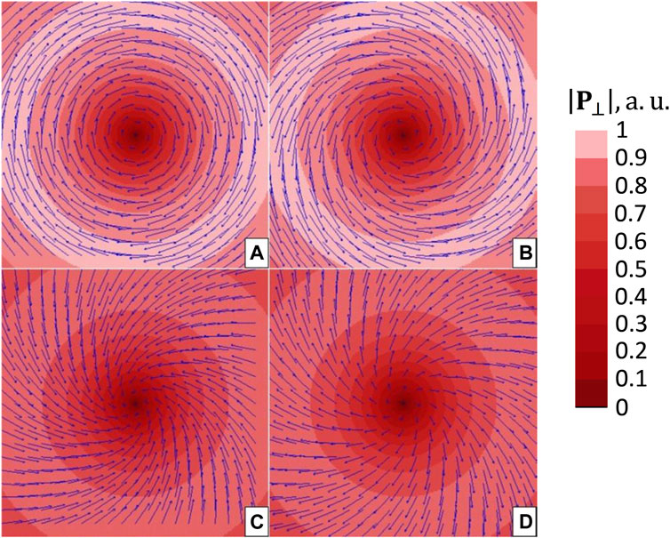
Figure 5. The structure of instantaneous energy flows (arrows) for the superposition (24) of linearly orthogonally polarized beams with different frequencies: a1x = a2y ≠ 0, a2x = a1y = 0, φ2y–φ1x = π/2, ω2 = 2ω1 (cf. Eqs 27). Images differ by the time moments t: (A) t = 0; (B) t = π/(ω2–ω1); (C) t = π/2 (ω2–ω1); (D) t = 3π/2 (ω2–ω1). The TPV structures in the second half-period (B, D) reproduce the mirror-reflected structures of the first half-period. The background of the panels (A–D) illustrate the TPV magnitude by the color saturation (see the colorbar).
Nevertheless, the instantaneous vortices similar to those depicted in Figure 5, like other optical vortices known from the literature [1, 58, 59, 69, 80–82], can be used for implementing the light-induced mechanical action on small particles, optical trapping and micromanipulation.
Presentation of the above Section 4 illustrates how the main concepts and approaches of the correlation optics, primary introduced for quasi-monochromatic fields with, generally, time-independent behavior of the main observable characteristics, can be extended to fields that are essentially non-stationary, and whose temporal evolution comprises their characteristic features important for the fields’ description and applications. Hence, we approach the intriguing and fascinating realm of spatio-temporal (ST) light fields where the temporal structure is of the main importance. This vivid branch of optical research started from the discovery of ultra-short pulses generated by lasers in the mode-locking regime (the history can be found in Ref. [83]), and shows the fruitful progress during the past decades, which was confirmed by the Nobel Prizes awarded in 2005, 2018 and 2023 [6]. Numerous captivating effects and impressive applications are described in a huge massive of literature (see, e.g., the recent compendia [2–5]), and the whole ST-optics domain cannot be properly reflected in the limited frame of this work. However, in this Section we present a few examples illustrating the productivity of the ideas of correlation and singular optics in this vibrant area of research.
First of all, we emphasize that in the ST optics, as well as for the stationary fields, the main way for extraction the optical-field parameters is the interference with a properly chosen reference wave. However, in case of ultra-short (femtosecond) pulses, the interference requires some special precautions. The main one is that the whole measurement process should be completed within the limited spatial and temporal duration of a single pulse (see [2], part 14); the second precaution is that both the object and reference waves are essentially polychromatic, and the interference pattern contains a “mixture” of overlapping monochromatic contributions, which implies the additional task of its deciphering and interpretation. These factors have led to the development of “single-shot spectral interference” (SSSI) schemes [84, 85] where the reference beam
In the arrangement of Figure 6A, the interference occurs in the 0.5 mm thick fused-silica “witness plate” where the Kerr effect produces the interference pattern. Regarding the regime, the interference signal is generated in the form
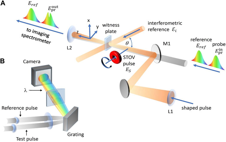
Figure 6. Setup for the single-shot spectral interference analysis: (A) three-beam Kerr-based SSSI for the STOV characterization [85]; (B) two-beam linear spectral interferometry (generalized scheme of Refs. [2, 86]). Further explanations see in text.
Another version of SSSI presented in Figure 6B involves only linear interactions [2, 86]. Here, the reference and sample (tested) pulses are collimated and spectrally resolved in the horizontal direction by the diffraction grating. The cylindrical lens projects the spectral distribution onto the camera input. In the vertical dimension, the reference and sample pulses’ trajectories cross at a small angle so that their images overlap at the camera thus forming the interference fringes. In this simple configuration, the spatial resolution is not high and is limited to the vertical direction only, but, using the beam-splitter, the same procedure can be simultaneously applied to the orthogonal transverse direction. Additionally, several copies of the sample pulse, with prescribed transverse shifts with respect to the reference position, can be analyzed simultaneously to improve resolution and signal-to-noise ratio.
In this way, the SSSI enables to obtain a spatially and spectrally resolved map of the sample-pulse field distribution. However, achievement of high spatial and spectral (temporal) resolution on a single-shot basis is still a challenge and its practical realization meets many difficulties, despite the crucial importance for high-power and low-repetition-rate laser systems.
Upon the conditions of Ref. [85], the SSSI is used for the experimental characterization of the ST optical vortex (STOV), which is a representative of a new family of singular ST light fields. Due to their unique physical properties, uniting the essential ST coupling with expressive topological and singular-optics features, the STOVs are in the focus of the most scrupulous and permanently growing attention during the last years [2, 3, 5, 85, 87–99]. Prior to discuss the physical properties and manifestations of the STOVs, we briefly outline their formal description.
To this purpose we start with considering the simplest Gaussian ST wave packet [100]. In the scalar paraxial approximation, its electric field distribution can be presented as
A is the normalization constant, and
where b0 is the beam waist radius, and it is supposed that the beam waist is situated at z = 0. Based on the wave packet (40), the usual (longitudinal) optical vortex (OV) can be constructed as
where σ = ±1 denotes the OV sign. Quite similarly, the STOV appears if the pre-exponential multiplier involves the spatial transverse (say, x) and longitudinal (temporal) s coordinates:
Like Eq. 42, this expression is a solution to the paraxial wave equation but its z-dependent evolution differs in some important aspects: in (42), the coefficients of x and y in the first parentheses evolve identically while in (43), the coefficient of x, exp (–iχ)/b varies according to the rules (41) but the coefficient of s remains constant. This stipulates peculiar features of the STOV propagation which are discussed below.
The properties of the STOV (43) are illustrated in Figure 7. The intensity distribution in the (x, s) plane, calculated for the case ζ = b0, σ = +1 and z = 0 (Figure 7A) is doughnut-shaped, with bright ring and dark spot in the center. Moreover, the isolated amplitude zero in point (s = 0, x = 0) is coupled with the phase singularity: the field phase is indeterminate at s = 0, x = 0, and grows by 2π upon the circulation near this point (Figure 7B). These features resemble the field pattern of a circular OV (42) in the transverse (x, y) plane depicted in Figure 7C for a comparison. The 3D spatial profile (instantaneous intensity distribution) of the STOV forms, generally, a toroidal structure that can be illustrated by the equal-intensity surfaces (Figures 7D–F). For the STOV (43), the toroid is situated in the longitudinal plane (s, x) containing the propagation axis [90, 95], while a light pulse with the conventional transverse OV forms a similar toroid in the (x, y) plane illustrated by Figure 7D; the “depth” of the latter toroid (its size along the s-direction) is determined by the pulse duration ζ/c.
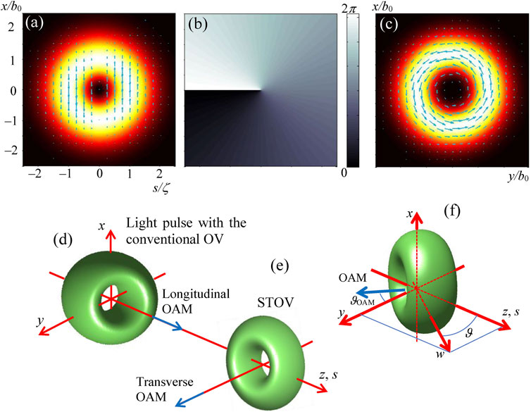
Figure 7. Characteristics of the STOV (43) with b0 = ζ = 0.1 mm,
The energy flows in the STOV are determined by Eq. 43 and the scalar versions of Eqs 33, 36 with k1 = k2 =
(w is the STOV energy density,
The TPV pattern in Figure 7A shows a sort of circulatory energy flow associated with the corresponding orbital angular momentum (OAM) of the STOV [90, 94–96]. It also resembles the OAM of a conventional OV (Figure 7C) but is directed orthogonally to the beam propagation (Figure 7E). Additional distinctions follow from the fact that the STOV (43) contains only the x-directed TPV component in the (s, x) plane. In contrast to the conventional circular OV (Figure 7C), in the STOV, a certain “imbalance” exists in the transverse energy flows between the regions s > 0 and s < 0, which is well seen in Figure 7A and Eqs. 45. Due to this imbalance, the spatial configuration of the STOV does not preserve the circular symmetry and changes in the course of propagation (see Figure 8).
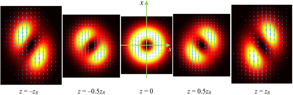
Figure 8. Spatial evolution of the STOV (43) with σ = 1 during propagation; for σ = −1, the patterns are mirror-reflected with respect to axis z (s). Other parameters are the same as in Figure 7.
As a result, the “perfect” circular STOV is only realized in a single cross section (under conditions of Figure 8, this is the waist section but proper adjustment of the parameters ζ, b0 and χ enables to get the circular STOV in any longitudinal location up to the far field [85]). In other cross sections, the intensity pattern is typical for the anisotropic (“non-canonical”) OV [20, 21, 101]. Ultimately, the energy-flow imbalance causes the intensity profile distortion, and the two-lobe structure appears. The whole evolution of the propagating STOV looks as a sort of rotation. The sense of this rotation is dictated by the sign of the STOV topological charge which is positive in Figure 8.
A STOV with the ring-like structure in a certain cross section z = z1 is described similarly to (43) with the only difference that the parameter ζ in the pre-exponential parentheses is replaced by the complex quantity
In general case, when
Like in the case of conventional OVs [58, 59, 80], the STOVs of any integer order l (also called topological charge) may exist, in which the phase increment on a circulation near the vortex center is 2πl. For a higher-order STOV, at least in a single cross section z = z1 the complex amplitude distribution can be represented as
where l = σ|l|. However, in other cross sections this simple form is destroyed: the pre-exponential binomial must be expanded in a series in degrees of (s/ζ), (x/b), and each summand evolves in its own way [94, 101]. This fact stipulates a rather rich and non-trivial picture of the STOV profile evolution, and enables purposeful formation of a necessary profile (e.g., ring-like one) at any specific position along the propagation axis up to the far field [85, 94].
The STOVs (43), (46), (47) considered so far are oriented such that their intensity toroids and the energy circulation are concluded within the plane (z, x) (see Figures 7A–E, 8). However, the STOVs with other toroid orientations may also exist [92]. For example, the following function is the solution of the ST paraxial wave equation [100]:
This STOV propagates along axis s but its equal-intensity toroid is adjusted along the plane (x, w) which is inclined at an angle ϑ (Figure 7F); the OAM orientation in the (z, y) plane is characterized by the angle ϑOAM which, generally, differs from ϑ. For example, if by = ζ, χy = 0 (conditions of Figure 7F) and α = β = 1/√2, ϑ = π/4. Practically, STOVs of arbitrary orientation can be realized [92].
It was already mentioned in comments to Eqs. 45 that the specific TPV distribution in the plane (x, s) is coupled with the transverse OAM with respect to any y-oriented axis. It is suitable to consider the OAM defined with respect to the moving axis (x = 0, s = 0) crossing the wave-packet center. Thus, the y-component of the Poynting vector gives no contribution, and the OAM density can be determined as
(cf. Eq. 39). The total OAM of the STOV is obtained via the integration of (49) over dxdyds. In this procedure, the term
In agreement with the angular momentum conservation, the result does not depend on z, despite that the pulse configuration changes rather impressively (as is seen, for example, in Figure 8). The quantity (50) depends on a set of the STOV parameters. However, like the longitudinal OAM of the conventional OV beams, the transverse OAM expresses the deep topological properties of the field which are largely “masked” by the specific parameters of the beam shape. To disclose this topological essence, the numerical OAM value (50) should be normalized by the beam energy. The total STOV energy is determined by the energy density distribution (44),
which, in view of Eq. 50, determines the OAM per unit energy of the STOV [95, 96]
where
It is instructive to compare this transverse OAM with the longitudinal OAM Λz of the conventional OV. In view of the generally astigmatic character of the STOV, for comparison we consider the light pulse with the astigmatic transverse OV, for which the longitudinal OAM Λz, normalized per unit energy, obeys the relation [96, 101]
where
This relation was the subject of a controversial discussion [95, 96] but it finds a simple qualitative support in juxtaposition of the corresponding energy flow patterns presented in Figures 7A, C [95]. The energy circulation in the conventional OV (Figure 7C) is “complete” and contains the “full” circulation including the contributions along both orthogonal transverse components while in the STOV field, only the ± x-oriented circulation contributions are present, so the circulation loses a half of its “complete” value.
There are several prospective approaches to the practical STOV generation discussed in literature [2, 91–93]. Conceptually, all of them employ one or several “source” light pulses without special structure, usually obtained from the mode-locked laser, which undergo certain structuring manipulations. In this regard, the most direct method is based on the superposition of properly prepared and phase-shifted non-vortex pulses, for example, those described by the first and second summands in pre-exponential parentheses of Eq. 43 [87]. In principle, this approach is applicable for obtaining any of the complicated STOV structures, e.g., characterized by Eqs 47, 48, as well as by their generalizations. But it requires preparing a number of special light pulses with prescribed configurations and their precise alignment, which is practically difficult.
Another group of approaches involves manipulations with the STOV Fourier-spectra,
where k = ω/c is the wavenumber corresponding to the spectral frequency ω, and
Such spectral density in the Fourier space
A sort of such transformation is implemented in the 2D pulse shaper [85, 90] (Figures 9A, B) where the general principle of “structuring light in time” ([3], part 21) is realized. Namely, the input dispersion element performs “spectrum-to-space” transformation such that different spectral components are spatially separated; ideally, each spectral component enters its own spatial channel. Then, in each channel, the prescribed modulation of the spatial (amplitude and phase) and, if appropriate, polarization distributions is executed, after which the spectral channels are recombined by another dispersion element operating in the inverse mode. The schemes of Figures 9A, B employ the simplified version of this principle. The dispersion elements are diffraction gratings that disperse the input wave packet components with different values of k along the horizontal direction. Then, in the cylindrical-lens focal plane, the complex amplitude distribution is formed proportional to
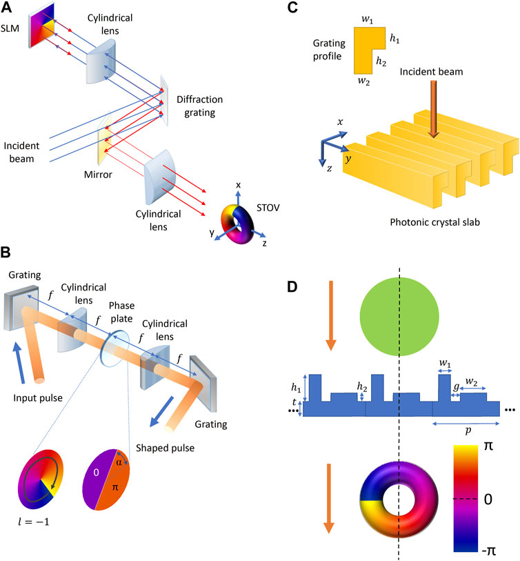
Figure 9. Examples of the STOV generation principles. (A, B) Beam-shaper schemes with (A) the reflecting SLM [90] and (B) phase plate [85] which introduce the spatio-spectral coupling (57) (β = 0) in the Fourier plane; the subsequent elements perform the inverse Fourier transform with the STOV formation at the prescribed longitudinal distance; (C) photonic-crystal grating with the spectral-depending transmittivity [92]; (D) ST differentiator with enhanced topological robustness [93] (additional explanations in text).
But the most universal approaches for the STOV generation involve the specially designed metasurfaces [92]. The main element of the corresponding arrangement (Figure 9C) is the photonic-crystal slab furnished with the grating formed of material with permittivity ε = 12 (the grating profile is shown by the yellow inset). The whole system is polarization-sensitive and is placed between the polarizers with prescribed input and output polarization. With specially adjusted sizes w1, w2, h1, h2 (see Figure 9C), very narrow Fano resonance is excited in the slab due to which its transmission for normally incident light of the central frequency
with, generally, complex coefficients ak and ax. The phase difference between ak and ax is determined by the slab properties and can be adjusted to π/2, which realizes the transmission function (57) with β = 0 responsible for the longitudinal STOV (43). The terms proportional to ky appear in the Taylor expansion if the slab is slightly tilted around the x- or y-axes, and in this manner the STOV with arbitrary orientation (see, e.g., Eq. 48) can be produced [92].
Other similar approaches employ other properties of specially designed nanostructures. For example, a ST differentiator based on 1D periodic silicon structure with two rods, of different heights and widths, per period (Figure 9D) has been used [93] to realize the transmission function (58) after which the STOV carrying transverse OAM appears immediately without special Fourier-transforming elements: the necessary transformations happen during free propagation of the pulse. The structure of nonlocal mirror-symmetry-breaking metasurface of Figure 9D is prospective for the STOV topological stability [91, 102]. Its properties can be regulated via the rod height h1: It was found that the phase singularity in the transmission spectrum only exists if h1 lies between 238.5 nm and 388.7 nm; in this case, the mirror symmetry is broken and phase singularities appear in pairs. For h1 within this range, the STOV can be generated with the structure stable to the metasurface random deviations and fabrication imperfections.
The specific features of the STOVs stipulate their possible applications in many areas. First of all, the STOVs can be employed for executing the functions traditionally associated with conventional longitudinal OVs, providing additional benefits of high speed and high energy concentration. They can be used for optical manipulation [103], free-space optical communications [104], in space-time differentiators [93], etc. The STOV has been successfully harnessed to manipulate light in nanostructures, to study the optical properties of molecular transparent media (e.g., for investigation of the molecular chirality [105]), and supply additional instruments for excitation and investigation of the light-matter interactions [91]. Using STOV, optical metrology of nonlinear media, as well as fast processing and transmission of information with intense concentration and release of energy are possible.
An important property of STOVs is the possibility to form the prescribed (ring-like or another) structure with the required ST behavior at a given propagation distance. In this regard, the attractive topic for future developments is the ability to control light in different dimensions and degrees of freedom. This is relevant when high-intensity light fields are assigned to control complex ST processes, such as plasma dynamics, dynamics of free electrons and X-ray radiation ([2], part 2). The problem arises of forming appropriate radiation sources in the form of a multimode nonlinear laser system that would organize and coordinate the light modes with the desired ST characteristics, and the STOVs can be helpful for its solution.
The non-trivial phase and topological structure of STOVs coupled with the high energy concentration opens interesting prospects in applications associated with the non-linear optical transformations [2]. In particular, in the processes of higher-harmonic generation, a possibility emerges to transform the structured light from infra-red to ultra-violet or X-ray diapason. A unique opportunity opens up to transfer the spin and orbital AM into ultrashort pulses of femtosecond to attosecond ranges [2, 106].
Important manifestations of the intrinsic coupling between the spatial and temporal properties of STOVs come to light in the processes of their reflection and refraction at a flat isotropic interface between two media. In this situation, in addition to the conventional Goos-Hänchen and Imbert-Fedorov shifts [107], a number of new spatial shifts and time delays are found, which are controlled by the value and orientation of the intrinsic optical AM [97]. In this approach, due to the special combination of spatial and temporal degrees of freedom in space-time vortices, time delays and spatial shifts occur without the frequency dependence of the reflection/refraction coefficients, and the “slow” and “fast” propagation of pulses can be realized without the medium dispersion. These results can be important for scattering of localized vortex states of light with the transverse AM, both in classical and quantum formulation [97].
An interesting version of the STOV, especially suitable due to relative simplicity of its generation, is the partially coherent STOV [108–111]. In contrast to other (coherent) STOVs, which are obtained using the source pulses of the mode-locking lasers, these wave packets originate from the amplified spontaneous emission or from the noise-like pulse states of the fiber laser. In such regimes, the source pulses show some stochastic features that can be modelled by a combination of randomly distributed spectral phase and a Gaussian spectrum profile. The coherence time τc of such fields exceeds the pulse duration
The use of the STOV as an information carrier is stipulated by the transverse OAM which adds an additional degree of freedom to the conventional OAM-based data-processing schemes [112]. Moreover, toroidal structures like those described in Figures 7D–F, are closely related to particle-like waves such as hopfions [113]. The latter can be considered as high-dimensional data-carriers whose employment for the information processing will increase the information dimension per pulse for optical communication [91].
The general overview of the correlation- and singular-optics approaches in the optical-diagnostic problems, presented in the above Sections, convincingly illustrates the intensive development and increasing influence of the optical science and technology in both fundamental and applied problems. It should be noted that, actually, the general topic, announced in the title, is practically spanless, and the limited frame of this paper prevent us from reflecting many important facts and data. Forcedly, we restrict ourselves to selected examples that are closest to the authors’ research interests and work experience.
Nevertheless, we hope that the materials presented in the current review supply distinct illustrations of the correlation-optics ideology and its development in the wider framework of singular and transient fields, e.g., non-monochromatic fields and localized wave packets. Below, we briefly summarize the main issues addressed in this review, the most important (to our understanding) subjects that are left beyond our scope, and some prospects of future development.
In many situations associated with the statistical analysis of singular light fields, the correlation properties of light can be considered as a sort of additional degree of freedom and additional channel of controllable light-matter interaction, which can be used, for example, in optical diagnostics of complex random objects, as is shown in Section 3.2 [52–54]. The corresponding opportunities constitute a base for several promising directions of research among which the peculiar interest is attracted by the rapidly developing branch of optical coherence tomography [114–118], especially useful in application to biological objects.
Another important direction of possible advances concerns the interrelations between the correlation optics and optical singularities. This topic has been briefly discussed in connection with the non-monochromatic ST fields, polarization beatings and transient energy flows (Section 4.2, Section 4.3). The important feature of singular optical fields is their topological nature dictating the stability of the qualitative field patterns and their robustness against external perturbations. Especially, singularities of the transverse energy flows are crucial for understanding the transient field patterns and principal mechanisms regulating the formation and evolution of observable time-averaged field characteristics. These issues are mainly fundamental; attractive application-oriented aspects associated with combination of the singular-optics and correlation-optics paradigms have been recently displayed in more detail [21].
Despite the multitude of novel branches of research and areas of application, which arise almost every day, the main traditional elements of the correlation and singular optics retain their fruitfulness and practical power. First of all, this relates to the principle of interference according to which the tested-field characteristics are obtained via its comparison with the time-delayed or spatially-shifted copy of the probing wave (the LCS approach described in Section 3.1.2 constitutes an exclusion but it puts increased demands on the probing-radiation stability and coherence). In this context, the most interesting, to our opinion, developments and applications of the correlation-optics techniques are associated with the vibrant area of structured ST optical fields, whose properties, description, methods of generation and applications are considered in Section 5. Simultaneously, some ingenious modifications of the correlation methods, adapted to ultra-short light pulses with ultra-wide spectral bands (including various versions of the single-shot spectral interferometry), are briefly outlined.
In order to focus on principles and to avoid inessential technical difficulties, in Section 5 the physical nature, theoretical foundations and experimental characterization of the ST fields have been presented, based mainly on the examples associated with Gaussian (in space and time) wave packets. Herewith, a number of other instructive and meaningful examples of the STOV fields have been inevitably missed. In particular, there should be mentioned the important family of Bessel STOVs [119, 120] which represent the ST version of the known Bessel-Gaussian beams [121] with the transverse OAM. Additionally, one cannot omit the very impressive class of “ST wave packets” which are also based on the Bessel beam model [4]. These optical structures demonstrate the unique propagation-invariant behavior: they can be “rigidly” transported in linear media preserving the spatial and temporal configuration during the whole evolution. Besides, these wave packets can be endowed with controllable group velocities in free space, showing both subluminal and superluminal propagation.
Furthermore, the analysis of the ST pulses has been restricted to the scalar approximation, which, enabling the simplified and pictorial demonstration of the principles governing the ST organization and evolution, neglects some fundamental details dictated by the vector nature of light waves. At the same time, it is the vector-based topological structures (toroidal and supertoroidal ST pulses, optical skyrmions, merons, hopfions, etc.) which attract the very intense and promising efforts of researchers ([2], part 11; [122–125]). Such optical structures are essentially singular and topologically determined. Their theoretical prototypes, being the exact solutions of the Maxwell equations, demonstrate the impressive fundamental features of light fields localized within a few oscillation cycles: 1) non-trivial vector nature with complex orientation of the electric and magnetic vectors; 2) fractal-like and self-similar singular building; 3) essential ST non-separability resulting in non-diffracting propagation over arbitrarily long distances; 4) expressive superoscillations [126] (i.e., the actual field oscillations occur with frequency higher than the highest spectral component). Toroidal and supertoroidal ST fields (also termed “flying doughnuts”) are so short that the usual time-averaged field characteristics, discussed in Section 4, are not applicable to them. Their instantaneous patterns show a rich set of singular textures in the electric and magnetic field distributions as well as in the instant energy flows; the regions of anomalous “back flow” may exist where the Poynting vector is directed oppositely to the direction of propagation [125]. These stable and robust topological structures are prospective for information encoding and transfer.
Very interesting and important features of the ST fields with singularities stem from their complex non-separable structure in space and time [127–129]. Investigations of such fields can be considered as the first step towards the formation of multidimensional structured light. In this process, the usual spatial degrees of freedom are supplemented by the time and spectral coordinates. Additionally, the light acquires specific degrees of freedom associated with the field vector directions and the internal energy flows, as well as stochastic ones associated with the spatial and temporal coherence [108–111]).
The development of complex light-shaping tools, as well as advances in nanotechnology will discover new ways to manipulate magnetic, molecular, and quantum excitations at the nanoscale with high resolution in four dimensions. In particular, the toroidal pulses are promising for the studies of subtle phenomena occurring at the frontier between classical and quantum optics, including the effects of quantum coherence and entanglement [130, 131].
In this regard, the recent achievements of the attosecond pulse techniques are especially exciting [2, 106]. Such pulses provide opportunities for observation and control of the electron processes inside atoms and molecules [6]. Their attractive physical features include the ability to carry OAM changing in time and accompanied by variation of their own momentum [106]; besides, trains of attosecond pulses can be created with controllable and variable pulse-by-pulse characteristics, e.g., polarization [132].
All these examples confirm the exceptional importance and necessity of further development of the singular and correlation optics in novel applications to highly structured light fields and material objects. Hopefully, this review will facilitate consistent and profitable advances in this direction.
OA: Conceptualization, Project administration, Supervision, Writing–original draft, Writing–review and editing. AB: Conceptualization, Methodology, Validation, Writing–original draft, Writing–review and editing. PM: Investigation, Methodology, Visualization, Writing–original draft, Writing–review and editing. IM: Data curation, Formal Analysis, Investigation, Writing–original draft, Writing–review and editing. CZ: Conceptualization, Data curation, Formal Analysis, Writing–original draft, Writing–review and editing. VG: Data curation, Investigation, Methodology, Writing–original draft, Writing–review and editing. DI: Investigation, Resources, Software, Writing–original draft, Writing–review and editing. JZ: Conceptualization, Funding acquisition, Resources, Supervision, Writing–original draft, Writing–review and editing.
The author(s) declare financial support was received for the research, authorship, and/or publication of this article. Research Institute of Zhejiang University—Taizhou, Center for Modern Optical Technology, China; Ministry of Education and Science of Ukraine (projects ## 0122U001830, 0122U001198).
The authors declare that the research was conducted in the absence of any commercial or financial relationships that could be construed as a potential conflict of interest.
All claims expressed in this article are solely those of the authors and do not necessarily represent those of their affiliated organizations, or those of the publisher, the editors and the reviewers. Any product that may be evaluated in this article, or claim that may be made by its manufacturer, is not guaranteed or endorsed by the publisher.
1. Angelsky OV, Bekshaev AY, Mokhun II, Vasnetsov MV, Zenkova CY, Hanson SG, et al. Review on the structured light properties: rotational features and singularities. Opto-Electronics Rev (2022) 30(2):e140860. doi:10.24425/opelre.2022.140860
2. Shen Y, Zhan Q, Wright LG, Christodoulides DN, Wise FW, Willner AE, et al. Roadmap on spatiotemporal light fields. J Opt (2023) 25(9):093001. doi:10.1088/2040-8986/ace4dc
3. Rubinsztein-Dunlop H, Forbes A, Berry MV, Dennis MR, Andrews DL, Mansuripur M, et al. Roadmap on structured light. J Opt (2017) 19(1):013001. doi:10.1088/2040-8978/19/1/013001
4. Yessenov M, Hall LA, Schepler KL, Abouraddy AF. Space-time wave packets. Adv Opt Photon (2022) 14(3):455–570. doi:10.1364/AOP.450016
5. Bliokh KY, Karimi E, Padgett MJ, Alonso MA, Dennis MR, Dudley A, et al. Roadmap on structured waves. J Opt (2023) 25(10):103001. doi:10.1088/2040-8986/acea92
6. The Nobel Prize in Physics. The Nobel prize in physics (2022). Available from: https://www.nobelprize.org/prizes/physics/ (Accessed May 24, 2024).
7. Wolf E. A macroscopic theory of interference and diffraction of light from finite sources. II. Fields with a spectral range of arbitrary width. Proc R Soc Lond (1955) 230:246–65. doi:10.1098/rspa.1955.0127
8. Wolf E, Shirai T, Agarwal G, Mandel L. Storage and retrieval of correlation functions of partially coherent fields. Opt Lett (1999) 24:367–36. doi:10.1364/OL.24.000367
9. Wolf E. Unified theory of coherence and polarization of random electromagnetic beams. Phys Lett A (2003) 312:263–7. doi:10.1016/S0375-9601(03)00684-4
10. Wolf E. Correlation-induced changes in the degree of polarization, the degree of coherence and the spectrum of random electromagnetic beams on propagation. Opt Lett (2003) 28:1078–80. doi:10.1364/OL.28.001078
12. Wolf E. Introduction to the theory of coherence and polarization of light. Cambridge: Cambridge University Press (2007).
13. Gbur G, Visser TD. The structure of partially coherent fields. Prog Opt (2010) 55:285–341. doi:10.1016/B978-0-444-53705-8.00005-9
14. Born M, Wolf E. Principles of optics: electromagnetic theory of propagation, interference and diffraction of light. Elsevier (2013).
15. Réfrégier P, Roueff A. Intrinsic coherence: a new concept in polarization and coherence theory OPN. Opt Photon News (2007) 18:30–5. doi:10.1364/OPN.18.2.000030
16. Setälä T, Tervo J, Friberg AT. Complete electromagnetic coherence in the space-frequency domain. Opt Lett (2004) 29:328–30. doi:10.1364/OL.29.000328
17. Ellis J, Dogariu A. Complex degree of mutual polarization. Opt Lett (2004) 29:536–8. doi:10.1364/OL.29.000536
18. Gori F. Matrix treatment for partially polarized, partially coherent beams. Opt Lett (1998) 23:241–3. doi:10.1364/OL.23.000241
19. Gori F, Vicalvi S, Borghi R, Guattari G. Beam coherence-polarization matrix. Pure Appl Opt (1998) 7:941–51. doi:10.1088/0963-9659/7/5/004
20. Mejıas PM, Martınez-Herrero R, Piquero G, Movilla JM. Parametric characterization of the spatial structure of non-uniformly polarized laser beams. Prog Quant Electron (2002) 26(2):65–130. doi:10.1016/S0079-6727(02)00003-4
21. Angelsky OV, Bekshaev AY, Zenkova CY, Ivansky DI, Zheng J. Correlation optics, coherence and optical singularities: basic concepts and practical applications. Front Phys (2022) 10:924508. doi:10.3389/fphy.2022.924508
22. Angelsky OV, Maksimyak PP. Polarization interferometry assessment of the water-lecithin system. Proc SPIE (1992) 1647:237–42. doi:10.1117/12.60211
23. Angelsky O, Maksimyak P, Rudeychuk V. Effect of phospholipids on intermolecular coupling in water. Proc SPIE (1993) 1922:105–10. doi:10.1117/12.146186
24. Zemskov EM, Seminogov VN, Yamnov AL. Microscopic theory of refractive index. Consideration of multiple scattering. Fiz Zhidk Sost (1982) 10:95–105.
25. Vikas D, Basu S, Dutta P. In-situ measurements of concentration and temperature during transient solidification of aqueous solution of ammonium chloride using laser interferometry. Int J Heat Mass Transf (2012) 55:2022–34. doi:10.1016/j.ijheatmasstransfer.2011.12.002
26. Abramov A, Dikov O, Ryabukho V, Shipovskaya A. Laser interferometry for study of mutual diffusion in polymer–solvent system. Proc SPIE (2006) 6165:61650F. doi:10.1117/12.696853
27. Bulavin LA, Gotsulskiy VY, Popov AY. Determination of characteristics of anomalous light scattering in the gradient solutions using electronic speckle-pattern interferometry control of concentration distribution. Ukr J Phys Opt (2014) 15:216–26. doi:10.3116/16091833/15/4/216/2014
28. Vuks MF. Light scattering in gases, liquids and solutions. Leningrad: Izdatel'stvo Leningradskogo Universiteta (1977). p. 320. (In Russian).
30. Dyrseth AA, Spooren R. Measuring mixing dynamics of transparent fluids with electronic speckle pattern interferometry. Appl Opt (1997) 36:6171–7. doi:10.1364/AO.36.006171
31. Mujeeb A, Nayar VU, Ravindran VR. Electronic Speckle Pattern Interferometry techniques for non-destructive evaluation: a review. Insight – Non-Destructive Test Condition Monit (2006) 48(5):275–81. doi:10.1784/insi.2006.48.5.275
32. Foord R, Jakeman E, Oliver CJ, Pike ER, Blagrove RJ, Wood E, et al. Determination of diffusion coefficients of haemocyanin at low concentration by intensity fluctuation spectroscopy of scattered laser light. Nature (1970) 227:242–5. doi:10.1038/227242a0
33. In: HZ Cummins, and ER Pike, editors. Photon correlation and light beating spectroscopy; NATO advanced study institutes series. Series B. Physics, v. 3. New York: Plenum Press (1974). p. 504.
34. Berne BJ, Pecora R. Dynamic light scattering with applications to chemistry. In: Biology and physics. New York: Willey-Interscience (1976).
35. In: W Brown, editor. Dynamic light scattering: the method and some applications. Oxford: Clarendon Press (1993).
36. "ISO 22412:2017. Particle size analysis — dynamic light scattering (DLS)". Geneva, Switzerland: ISO https://cdn.standards.iteh.ai/samples/65410/d885a552582f401894bc1dc4449e7f3e/ISO-22412-2017.pdf. Retrieved 31 May 2022.
37. Zaremba VG, Salistra GI, Gotsulskiy VY, Chechko VE. Determination of higher moments of correlation functions of electromagnetic fields with a one-point registration. Ukr J Phys (1995) 40(6):638–9. (in Ukrainian).
38. Gotsul'skij VY, Chechko VE, Zaremba VG. Correlometer of pulse random signals. Pribory i Tekhnika Eksperimenta (1997) 2:101–2.
39. Gotsulskiy VY, Chechko VE, Melnik YA. The origin of light scattering by aqueous solutions of alcohols in vicinities of their singular points. Ukr J Phys (2015) 60:780. doi:10.15407/ujpe60.08.0782
40. Chechko VY, Gotsulskiy VY, Malomuzh NP. Peculiar points of aqueous solutions of mono-hydrogen alcohols. J Mol Liq (2022) 367:120537. doi:10.1016/j.molliq.2022.120537
41. Smirnova DA, Nori F, Bliokh KY. Water-wave vortices and skyrmions. Phys Rev Lett (2024) 132(5):054003. doi:10.1103/PhysRevLett.132.054003
42. Bliokh KY, Punzmann H, Xia H, Nori F, Shats M. Field theory spin and momentum in water waves. Sci Adv (2022) 8(3):eabm1295. doi:10.1126/sciadv.abm1295
43. Chen J, Ji B, Lang P, Zhang Y, Lin J. Impact of the geometry of the excitation structure on optical skyrmion. Opt Express (2023) 31:37929–42. doi:10.1364/OE.500291
44. Rytov SM, Kravtsov YA, Tatarskii VI Principles of statistical radiophysics: elements of random fields, 3. Berlin: Springer (1989). p. 115.
45. Andrews LC, Phillips RL, Weeks AR. Propagation of a Gaussian-beam wave through a random phase screen. Waves in Random Media (1997) 7(2):229–44. doi:10.1088/0959-7174/7/2/005
46. Jakeman E, Pusey PN. Non-Gaussian fluctuations in electromagnetic radiation scattered by random phase screen. I. Theory. J Phys A: Math Gen (1975) 8(3):369–91. doi:10.1088/0305-4470/8/3/010
47. Angelsky OV, Bekshaev AY, Zenkova CY, Ivansky DI, Zheng J, Tkachuk VM. Fluorescence record diagnostics of 3D rough-surface landscapes with nano-scale inhomogeneities. Front Phys (2022) 9:787821. doi:10.3389/fphy.2021.787821
48. Angelsky OV, Maksimyak PP. Optical diagnostics of random phase objects. Appl Opt (1990) 29:2894–8. doi:10.1364/AO.29.002894
49. Angelsky OV, Maksimyak PP. Optical diagnostics of slightly rough surfaces. Appl Opt (1992) 31:140–3. doi:10.1364/AO.31.000140
50. Angelsky OV, Maksimyak PP, Ryukhtin VV, Hanson SG. New feasibilities for characterizing rough surfaces by optical-correlation techniques. Appl Opt (2001) 40:5693–707. doi:10.1364/AO.40.005693
51. Angelsky OV, Burkovets DN, Maksimyak PP, Hanson SG. Applicability of the singular-optics concept for diagnostics of random and fractal rough surfaces. Appl Opt (2003) 42:4529–40. doi:10.1364/AO.42.004529
52. Angelsky OV, Hanson SG, Maksimyak AP, Maksimyak PP. Interference diagnostics of white-light vortices. Opt Express (2005) 13:8179–83. doi:10.1364/OPEX.13.008179
53. Angelsky OV, Maksimyak AP, Maksimyak PP, Hanson SG. Optical correlation diagnostics of rough surfaces with large surface inhomogeneities. Opt Express (2006) 14:7299–311. doi:10.1364/OE.14.007299
54. Angelsky OV, Hanson SG, Maksimyak PP The use of optical-correlation techniques for characterizing scattering object and media, PM71. Bellingham: SPIE Press (1999).
55. Angelsky OV, Zenkova CY, Hanson SG, Ivansky DI, Tkachuk VM, Zheng J. Random object optical field diagnostics by using carbon nanoparticles. Opt Express (2021) 29:916–28. doi:10.1364/OE.411118
56. Kendall MG, Stuart A. The advanced theory of statistics. In: Distribution theory, Vol. 1. London: Griffin Co. Ltd. (1960).
57. Mokhun I, Bodyanchuk I, Galushko K, Yu G, Yu V. Formation mechanisms of the averaged Poynting vector of a polychromatic wave. Opt Mem Neural Netw (2021) 30:312–26. doi:10.3103/S1060992X2104010X
58. Bekshaev A, Bliokh K, Soskin M. Internal flows and energy circulation in light beams. J Opt (2011) 13(5):053001. doi:10.1088/2040-8978/13/5/053001
59. Angelsky OV, Bekshaev AY, Hanson SG, Zenkova CY, Mokhun II, Zheng J. Structured light: ideas and concepts. Front Phys (2020) 8:114. doi:10.3389/fphy.2020.00114
60. Angelsky O, Bekshaev A, Zenkova C, Ivanskyi C, Maksymyak P, Kryvetsky V, et al. Application of the luminescent carbon nanoparticles for optical diagnostics of structure-inhomogeneous objects at the micro- and nanoscales. Opt Mem Neural Netw (2023) 32:258–74. doi:10.3103/S1060992X23040069
61. Mandel L, Wolf E. Coherence properties of optical fields. Rev Mod Phys (1965) 37(2):231–87. doi:10.1103/RevModPhys.37.231
62. Kessler DA, Freund I. Lissajous singularities. Opt Lett (2003) 28:111–3. doi:10.1364/ol.28.000111
63. Freund I. Bichromatic optical Lissajous fields. Opt Commun (2003) 226:351–76. doi:10.1016/j.optcom.2003.07.053
64. Fleischer A, Kfir O, Diskin T, Sidorenko P, Cohen O. Spin angular momentum and tunable polarization in high-harmonic generation. Nat Photon (2014) 8:543–9. doi:10.1038/nphoton.2014.108
65. Pisanty E, Machado GJ, Vicuña-Hernández V, Picón A, Celi A, Torres JP, et al. Knotting fractional-order knots with the polarization state of light. Nat Photon (2019) 13:569–74. doi:10.1038/s41566-019-0450-2
66. Miao W, Visser TD, Gbur G. Lissajous singularities in Young’s interference experiment. Opt Express (2024) 32:813–24. doi:10.1364/oe.510413
68. Anan'ev YA, Bekshaev AY. Theory of intensity moments for arbitrary light beams. Opt Spectrosc (1994) 76(4):558–68.
69. Dennis MR, O'Holleran K, Padgett MJ. Chapter 5 singular optics: optical vortices and polarization singularities. Prog Opt (2009) 53:293–363. doi:10.1016/S0079-6638(08)00205-9
70. Angelsky OV, Mokhun II, Bekshaev AY, Zenkova CY, Zheng J. Polarization singularities: topological and dynamical aspects. Front Phys (2023) 11:1147788. doi:10.3389/fphy.2023.1147788
71. Mokhun I, Bodyanchuk I, Ye K, Turubarova-Leunova N. Characteristics of a field formed by superposition of two plane waves with different frequencies and different polarization. Proc SPIE (2018):10612. doi:10.1117/12.2304786
72. Mokhun I, Bodyanchuk I. Polarization characteristics of a polychromatic wave. Ukr J Phys Opt (2022) 23:30–6. doi:10.3116/16091833/23/1/30/2022
73. Gil JJ, Norrman A, Friberg AT, Setälä T. Spin of random stationary light. Phys Rev A (2023) 107(5):053518. doi:10.1103/PhysRevA.107.053518
74. Shen Y. Rays, waves, SU (2) symmetry and geometry: toolkits for structured light. J Opt (2021) 23:124004. doi:10.1088/2040-8986/ac3676
76. Bekshaev AY, Soskin MS, Vasnetsov MV. Angular momentum of a rotating light beam. Opt Commun (2005) 249:367–78. doi:10.1016/j.optcom.2005.01.046
77. Bekshaev A. Bi-chromatic paraxial beam as a representative of spatio-temporal light fields: modeling abilities and restrictions. Proc SPIE (2024):12938. doi:10.1117/12.3009856
78. Zhao Z, Song H, Zhang R, Pang K, Liu C, Song H, et al. Dynamic spatiotemporal beams that combine two independent and controllable orbital-angular-momenta using multiple optical-frequency-comb lines. Nat Commun (2020) 11:4099. doi:10.1038/s41467-020-17805-1
79. Mokhun I, Bodyanchuk I, Galushko K, Galushko Y, Val O, Viktorovskaya Y. Energy flows in polychromatic fields. J Opt (2021) 23:015401. doi:10.1088/2040-8986/abcc54
80. Soskin MS, Vasnetsov MV. Singular optics. Prog Opt (2001) 42(4):219–76. doi:10.1016/S0079-6638(01)80018-4
81. Bowman RW, Padgett MJ. Optical trapping and binding. Rep Prog Phys (2013) 76(2):026401. doi:10.1088/0034-4885/76/2/026401
82. Shen Y, Wang X, Xie Z, Min C, Fu X, Liu Q, et al. Optical vortices 30 years on: OAM manipulation from topological charge to multiple singularities. Light Sci Appl (2019) 8:90. doi:10.1038/s41377-019-0194-2
83. Haus HA. Mode-locking of lasers. IEEE J Sel Top Quan Electron (2000) 6(6):1173–85. doi:10.1109/2944.902165
84. Kim KY, Alexeev I, Milchberg HM. Single-shot supercontinuum spectral interferometry. Appl Phys Lett (2002) 81:4124–6. doi:10.1063/1.1524701
85. Hancock SW, Zahedpour S, Goffin A, Milchberg HM. Free-space propagation of spatiotemporal optical vortices. Optica (2019) 6:1547–53. doi:10.1364/OPTICA.6.001547
86. Bowlan P, Gabolde P, Trebino R. Directly measuring the spatio-temporal electric field of focusing ultrashort pulses. Opt Express (2007) 15:10219–30. doi:10.1364/OE.15.010219
87. Sukhorukov AP, Yangirova VV. Spatio-temporal vortices: properties, generation and recording. Proc SPIE (2005) 5949:35–43. doi:10.1117/12.623906
88. Bliokh KY, Nori F. Spatiotemporal vortex beams and angular momentum. Phys Rev A (2012) 86:033824. doi:10.1103/PhysRevA.86.033824
89. Jhajj N, Larkin I, Rosenthal EW, Zahedpour S, Wahlstrand JK, Milchberg HM. Spatiotemporal optical vortices. Phys Rev (2016) 6:031037. doi:10.1103/PhysRevX.6.031037
90. Chong A, Wan C, Chen J, Zhan Q. Generation of spatiotemporal optical vortices with controllable transverse orbital angular momentum. Nat Photon (2020) 14(6):350–4. doi:10.1038/s41566-020-0587-z
91. Wan C, Chong A, Zhan Q. Optical spatiotemporal vortices. eLight (2023) 3(1):11–3. doi:10.1186/s43593-023-00042-6
92. Wang H, Guo C, Jein W, Song AY, Fan S. Engineering arbitrarily oriented spatiotemporal optical vortices using transmission nodal lines. Optica (2021) 8:966–71. doi:10.1364/OPTICA.426460
93. Huang J, Zhang J, Zhu T, Ruan Z. Spatiotemporal differentiators generating optical vortices with transverse orbital angular momentum and detecting sharp change of pulse envelope. Laser Photonics Rev (2022) 16:2100357. doi:10.1002/lpor.202100357
94. Hancock SW, Zahedpour S, Milchberg HM. Mode structure and orbital angular momentum of spatiotemporal optical vortex pulses. Phys Rev Lett (2021) 127(19):193901. doi:10.1103/physrevlett.127.193901
95. Porras MA. Transverse orbital angular momentum of spatiotemporal optical vortices. Prog Electromagn Res (2023) 177:95–105. doi:10.2528/PIER23012203
96. Bliokh K. Orbital angular momentum of optical, acoustic, and quantum-mechanical spatiotemporal vortex pulses. Phys Rev A (2023) 107:L031501. doi:10.1103/PhysRevA.107.L031501
97. Mazanov M, Sugic D, Alonso M, Nori F, Bliokh KY. Transverse shifts and time delays of spatiotemporal vortex pulses reflected and refracted at a planar interface. Nanophotonics (2021) 11(4):737–44. doi:10.1515/nanoph-2021-0294
98. Bliokh KY. Spatiotemporal vortex pulses: angular momenta and spin-orbit interaction. Phys Rev Lett (2021) 126:243601. doi:10.1103/PhysRevLett.126.243601
99. Hancock SW, Zahedpour S, Goffin A, Milchberg HM. Spatio-temporal optical vortex (STOV) pulses. Proc SPIE (2023):12436. doi:10.1117/12.2652132
100. Porras MA. Ultrashort pulsed Gaussian light beams. Phys Rev E (1998) 58(1):1086–93. doi:10.1103/PhysRevE.58.1086
101. Bekshaev AY, Karamoch AI. Astigmatic telescopic transformation of a high-order optical vortex. Opt Commun (2008) 281:5687–96. doi:10.1016/j.optcom.2008.09.017
102. Huang J, Zhang H, Wu B, Zhu T, Ruan Z. Topologically protected generation of spatiotemporal optical vortices with nonlocal spatial mirror symmetry breaking metasurface. Phys Rev B (2023) 108:104106. doi:10.1103/PhysRevB.108.104106
103. Stilgoe AB, Nieminen TA, Rubinsztein-Dunlop H. Controlled transfer of transverse orbital angular momentum to optically trapped birefringent microparticles. Nat Photon (2022) 16:346–51. doi:10.1038/s41566-022-00983-3
104. Wang J. Advances in communications using optical vortices. Photon Res (2016) 4:B14–28. doi:10.1364/PRJ.4.000B14
105. Ni J, Liu S, Wu D, Lao Z, Wang Z, Huang K, et al. Gigantic vortical differential scattering as a monochromatic probe for multiscale chiral structures. Proc Natl Acad Sci (2021) 118:e2020055118. doi:10.1073/pnas.2020055118
106. Shi X, Liao CT, Tao Z, Cating-Subramanian E, Murnane MM, Hernández-García C, et al. Attosecond light science and its application for probing quantum materials. J Phys B: Mol Opt Phys (2020) 53:184008. doi:10.1088/1361-6455/aba2fb
107. Bliokh KY, Aiello A. Goos–Hänchen and Imbert–Fedorov beam shifts: an overview. J Opt (2013) 15:014001. doi:10.1088/2040-8978/15/1/014001
108. Hyde MW. Twisted space-frequency and space-time partially coherent beams. Sci Rep (2020) 10:12443. doi:10.1038/s41598-020-68705-9
109. Mirando A, Zang Y, Zhan Q, Chong A. Generation of spatiotemporal optical vortices with partial temporal coherence. Opt Express (2021) 29:30426–35. doi:10.1364/OE.431882
110. Ding C, Horoshko D, Korotkova O, Jing C, Qi X, Pan L. Source coherence-induced control of spatiotemporal coherency vortices. Opt Express (2022) 30:19871–88. doi:10.1364/OE.458666
111. Ding C, Liang C, Horoshko D, Korotkova O, Pan L, Liu Z. Method for generating spatiotemporal coherency vortices and spatiotemporal dislocation curves. Opt Express (2024) 32:609–24. doi:10.1364/OE.509764
112. Bozinovic N, Yue Y, Ren Y, Tur M, Kristensen P, HuangWillner HA, et al. Terabit-scale orbital angular momentum mode division multiplexing in fibers. Science (2013) 340:1545–8. doi:10.1126/science.1237861
113. Wan C, Shen Y, Chong A, Zhan Q. Scalar optical hopfions. eLight (2022) 2:22–7. doi:10.1186/s43593-022-00030-2
114. Huang D, Swanson EA, Lin CP, Schuman JS, Stinson WG, Chang W, et al. Optical coherence tomography. Science (1991) 254:1178–81. doi:10.1126/science.1957169
115. de Freitas AZ, Amaral MM, Raele MP. Optical coherence tomography: development and applications. In: FG Duarte, editor. Laser pulse phenomena and applications. Rijeka, Croatia: IntechOpen (2010). p. 409–32. doi:10.5772/12899
116. Aumann S, Donner S, Fischer J, Mǘller F. Optical coherence tomography (OCT): principle and technical realization. In: JF Bille, editor. High resolution imaging in microscopy and ophthalmology. Cham: Springer (2019). p. 59–85. doi:10.1007/978-3-030-16638-0_3
117. Everett M, Magazzeni S, Schmoll T, Kempe M. Optical coherence tomography: from technology to applications in ophthalmology. Translational Biophotonics (2021) 3:e202000012. doi:10.1002/tbio.202000012
118. Angelsky OV, Bekshaev AY, Zenkova CY, Ivanskyi DI, Zheng J, Chumak MM. Modeling of the high-resolution optical-coherence diagnostics of birefringent biological tissues. Front Phys (2023) 11:1260830. doi:10.3389/fphy.2023.1260830
119. Dallaire M, McCarthy N, Piché M. Spatiotemporal Bessel beams: theory and experiments. Opt Express (2009) 17:18148–64. doi:10.1364/OE.17.018148
120. Cao Q, Chen J, Lu K, Wan C, Chong A, Zhan Q. Non-spreading Bessel spatiotemporal optical vortices. Sci Bull (2022) 67:133–40. doi:10.1016/j.scib.2021.07.031
121. Borghi R, Santarsiero M, Porras MA. Nonparaxial bessel-gauss beams. J Opt Soc Am A (2001) 18:1618–26. doi:10.1364/JOSAA.18.001618
122. Shen Y, Hou Y, Papasimakis N, Zheludev NI. Supertoroidal light pulses as electromagnetic skyrmions propagating in free space. Nat Commun (2021) 12:5891. doi:10.1038/s41467-021-26037-w
123. Zdagkas A, McDonnell C, Deng J, Shen Y, Li G, Ellenbogen T, et al. Observation of toroidal pulses of light. Nat Photon (2022) 16(7):523–8. doi:10.1038/s41566-022-01028-5
124. Shen Y, Zhang Q, Shi P, Du L, Yuan X, Zayats AV. Optical skyrmions and other topological quasiparticles of light. Nat Photon (2024) 18:15–25. doi:10.1038/s41566-023-01325-7
125. Zdagkas A, Papasimakis N, Savinov V, Dennis MR, Zheludev NI. Singularities in the flying electromagnetic doughnuts. Nanophotonics (2019) 8:1379–85. doi:10.1515/nanoph-2019-0101
126. Berry M, Zheludev N, Aharonov Y, Colombo F, Sabadini I, Struppa DC, et al. Roadmap on superoscillations. J Opt (2019) 21(2019):053002. doi:10.1088/2040-8986/ab0191
127. He C, Shen Y, Forbes A. Towards higher-dimensional structured light. Light Sci Appl (2022) 11:205. doi:10.1038/s41377-022-00897-3
128. Shen Y, Zdagkas A, Papasimakis N, Zheludev NI. Measures of space-time nonseparability of electromagnetic pulses. Phys Rev Res (2021) 3(1):013236. doi:10.1103/PhysRevResearch.3.013236
129. Shen Y, Rosales-Guzmán C. Nonseparable states of light: from quantum to classical. Laser Photon Rev (2022) 16:2100533. doi:10.1002/lpor.202100533
130. Forbes A, Nape I. Quantum mechanics with patterns of light: progress in high dimensional and multidimensional entanglement with structured light AVS Quantum Sci. AVS Quan Sci (2019) 1:011701. doi:10.1116/1.5112027
131. Yan Q, Hu X, Fu Y, Lu C, Fan C, Liu Q, et al. Quantum topological photonics. Adv Opt Mater (2021) 9:2001739. doi:10.1002/adom.202001739
132. Dorney KM, Ellis JL, Hernández-García C, Hickstein DD, Mancuso CA, Brooks N, et al. Helicity-selective enhancement and polarization control of attosecond high harmonic waveforms driven by bichromatic circularly polarized laser fields. Phys Rev Lett (2017) 119(6):063201. doi:10.1103/PhysRevLett.119.063201
Keywords: correlation optics, coherence, aqueous-solution diagnostics, optical singularity, random phase object, polychromatic light, internal energy flows, spatio-temporal optical vortex
Citation: Angelsky OV, Bekshaev AY, Maksimyak PP, Mokhun II, Zenkova CY, Gotsulskiy VY, Ivanskyi DI and Zheng J (2024) Correlation and singular optics for diagnostics of structured light and condensed matter: time-stationary and spatio-temporal approaches. Front. Phys. 12:1383256. doi: 10.3389/fphy.2024.1383256
Received: 07 February 2024; Accepted: 10 May 2024;
Published: 10 June 2024.
Edited by:
Yuxuan Ren, Fudan University, ChinaReviewed by:
Daryl Preece, University of California, Irvine, United StatesCopyright © 2024 Angelsky, Bekshaev, Maksimyak, Mokhun, Zenkova, Gotsulskiy, Ivanskyi and Zheng. This is an open-access article distributed under the terms of the Creative Commons Attribution License (CC BY). The use, distribution or reproduction in other forums is permitted, provided the original author(s) and the copyright owner(s) are credited and that the original publication in this journal is cited, in accordance with accepted academic practice. No use, distribution or reproduction is permitted which does not comply with these terms.
*Correspondence: Jun Zheng, ZGJ6akBuZXRlYXNlLmNvbQ==
Disclaimer: All claims expressed in this article are solely those of the authors and do not necessarily represent those of their affiliated organizations, or those of the publisher, the editors and the reviewers. Any product that may be evaluated in this article or claim that may be made by its manufacturer is not guaranteed or endorsed by the publisher.
Research integrity at Frontiers
Learn more about the work of our research integrity team to safeguard the quality of each article we publish.