Intelligent Bayesian regularization backpropagation neuro computing paradigm for state features estimation of underwater passive object

In underwater environments, the accurate estimation of state features for passive object is a critical aspect of various applications, including underwater robotics, surveillance, and environmental monitoring. This study presents an innovative neuro computing approach for instantaneous state features reckoning of passive marine object following dynamic Markov chains. This paper introduces the potential of intelligent Bayesian regularization backpropagation neuro computing (IBRBNC) for the precise estimation of state features of underwater passive object. The proposed paradigm combines the power of artificial neural network with Bayesian regularization technique to address the challenges associated with noisy and limited underwater sensor data. The IBRBNC paradigm leverages deep neural networks with a focus on backpropagation to model complex relationships in the underwater environment. Furthermore, Bayesian regularization is introduced to incorporate prior knowledge and mitigate overfitting, enhancing the model’s robustness and generalization capabilities. This dual approach results in a highly adaptive and intelligent system capable of accurately estimating the state features of passive object in real-time. To evaluate the efficacy of this intelligent computing approach, a controlled supervised maneuvering trajectory for underwater passive object is constructed. Real-time estimations of location, velocity, and turn rate for dynamic target are scrutinized across five distinct scenarios by varying the Gaussian observed noise’s standard deviation, aiming to minimize mean square errors (MSEs) between real and estimated values. The effectiveness of the proposed IBRBNC paradigm is demonstrated through extensive simulations and experimental trials. Results showcase its superiority over traditional nonlinear filtering methods like interacting multiple model extended Kalman filter (IMMEKF) and interacting multiple model unscented Kalman filter (IMMUKF), especially in the presence of noise, incomplete measurements and sparse data.

1 Introduction

The estimation of state elements for passive vehicles in aquatic environments poses a significant challenge and is of utmost importance for a wide range of applications [1]. The usages of these technologies incorporate several fields, including underwater robotics, where accurate knowledge of a vehicle’s trajectory and orientation is essential. As well as surveillance, which requires the tracking of targets of interest, and atmosphere monitoring, where identifying the complexities of marine ecosystems is of extreme importance [2, 3]. Accurately forecasting the state characteristics of passive object is a crucial factor in various circumstances, as it directly impacts its efficiency and safety of operations [4]. One of the main challenges in estimating the state features of submerged object is the inherent noise and limited availability of sensor data in aquatic scenarios [5]. In the domain of underwater sensing, many types of sensors, including sonar, acoustic, and optical sensors, frequently encounter a wide range of noise sources arising from phenomena such as water turbulence, ambient noise, and signal compression [6]. These elements have a tendency to provide measurement errors, hence posing challenges in the extraction of useful information for the state estimation mechanism. In addition, underwater processes often face situations in which there may be a lack of sensor coverage, demanding the development of creative approaches to address data deficiencies [7]. State estimation is a crucial aspect within the field of underwater robotics as it facilitates the ability of autonomous underwater vehicles (AUVs) to navigate, execute tasks, and successfully engage with their surrounding water [8]. Precise assessments of a vehicle’s physical coordinates, speed, and angular orientation are crucial for various activities, including subaquatic mapping, investigation, and even archaeological research. The capability of accurately evaluating these state characteristics in real-time and adapt to varying underwater conditions is a vital requirement for the effective execution of underwater robotic activities [9].

Researchers have been actively investigating novel methods for estimating state features in order to address the challenges presented by complex underwater mediums [10]. The utilization of well-known Kalman filtering and its nonlinear versions holds considerable importance for estimating the current state of underwater objects [11]. The employing of filtering techniques is vital in the process of modeling and estimating the state features of passive targets within underwater environments. The Kalman filter (KF), along with its derivative methods such as the extended Kalman filter (EKF) and unscented Kalman filter (UKF) demonstrates exceptional proficiency in state estimation through effective handling of measurements affected by noise. These filtering algorithms deploy probabilistic models in order to make estimations about the condition of submerged targets, thereby mitigating the impact of noise and yielding more precise estimations [12]. Most state feature estimation problems in underwater environments consist of non-linear correlations among state parameters and measurements [13]. In instances of this nature, conventional linear KFs are not properly viable. The EKF and UKF are algorithms that have been developed with the explicit purpose of mitigating the effects of nonlinearity in system models [14]. This is achieved by approximating the nonlinear system dynamics through linearization at each discrete time step. The aforementioned capacity enables them to effectively manage a diverse set of underwater target motion models and measurement expressions, hence improving the accuracy of state feature estimation [15]. Underwater circumstances exhibit dynamic behaviors, characterized by the presence of quickly fluctuating conditions, including underwater currents, tides, and object maneuverings. In this situation, the adaptable nature of KF and its nonlinear versions is essential [16]. One of the primary constraints associated with the EKF and UKF methodologies is their underlying assumption of linearity. There are a lot of underwater target tracking circumstances where state variables and measurements have nonlinear associations. In cases, where the system exhibits substantial nonlinearity, the application of these filters for linearization purposes may result in inaccuracies, resulting in imprecise state feature estimations. Accurately simulating these processes can be challenging in underwater environments, where the dynamics can be complicated and unpredictable [17].

The utilization of interacting multiple model (IMM) Kalman filtering is of great importance in the assessment of the state of underwater targets, especially in situations where the dynamics of the target or the underwater environment are prone to frequent alterations or uncertainty [18]. This modified filtering strategy aims to mitigate certain drawbacks inherent in conventional Kalman filtering approaches, hence providing numerous benefits [19]. The IMM Kalman filtering technique enables the representation of numerous motion models or modes, each characterizing a distinct target behavior. IMM Kalman filtering demonstrates exceptional performance in tracking dynamic behaviors shown by underwater targets that exhibit motion pattern variations, such as dodging maneuvers or alterations in depth [20]. The technique has the capability to smoothly transition between various motion models in order to uphold precise state estimation. The selection of motion models in the context of IMM Kalman filtering is often a complex decision-making process [21]. The task of choosing an appropriate combination of models and their associated transition probabilities might present difficulties, as it relies on the particular behavior of the undersea target, which may not always be fully known or readily described [22]. The selection of inappropriate models can result in poor results, filter divergence, and overfitting. Moreover, the inclusion of a large number of models may lead to the formation of a system that is overly complicated without necessarily enhancing the accuracy of state features estimation [23]. When dealing with instances where the undersea target exhibits extreme, sudden, or erratic fluctuations in behavior, IMM Kalman filtering may encounter challenges in fast transitioning between models or precisely adjusting to these changes [24]. The integration of neural networks and deep learning has demonstrated potential for improving the precision and flexibility of state estimation mechanisms in the underwater domain [25]. The use of deep learning techniques in state feature estimation of underwater objects has experienced a significant rise, bringing about an evolutionary effect. This is primarily attributed to deep learning’s capacity to effectively process complicated data, dynamically adjust to varying underwater conditions, and deliver precise estimations [26]. Deep learning models, specifically convolutional neural networks (CNNs) and recurrent neural networks (RNNs), have exceptional proficiency in independently extracting relevant information from raw sensor input, including acoustic sonar, and visualizing data [27, 28]. The collection of these learned parameters is crucial in the description of the submerged surroundings and the movement of objects, hence enhancing the precision of state feature estimates. Often, in underwater environments, the relationships between sensor readings and target states are highly nonlinear. Deep learning models possess a built-in capacity to effectively capture and represent nonlinearities, hence enabling more precise state feature estimation in comparison to conventional nonlinear variants of KF [29]. Due to several reasons such as obstacles, noise, or constraints in the sensors, underwater data may be sparse and unstable. Deep learning models have the ability to efficiently address the challenges posed by missing data points and inconsistent measurements through the utilization of time series and historical data [30]. These methods provide the capability to dynamically adjust the new data in real-time, enabling them to effectively handle unknown variations in the undersea environment or the behavior of the target [31]. This adaptability is of great significance in order to ensure precise state estimations while circumstances undergo changes.

Intelligent Bayesian regularization backpropagation neuro computing (IBRBNC) is a category of artificial neural networks (ANNs) that integrate Bayesian methods for regularization [32]. It has proven useful in a wide range of situations, especially when working with sparse data or in a noisy environment. The IBRBNC method offers a probabilistic structure that allows the modeling of uncertainties in predictions made by neural network [33]. These systems possess the ability to adapt their complexity according to the quantity of accessible data, making them highly suitable for various applications that exhibit dynamic data features. The effectiveness of IBRBNC has been found in various financial applications, including but not limited to stock price forecasting, risk evaluation, and portfolio optimization [34]. This innovation has the potential to facilitate disease diagnosis, evaluate patient risk levels, and provide recommendations for therapy treatments. The capacity to offer estimations of uncertainty can aid medical professionals in making well-informed judgments [35]. The IBRBNC extends across many domains, encompassing cybersecurity, network surveillance, and manufacturing quality control [36]. This soft computing has been employed in several natural language processing applications, including sentiment detection, text sorting, and machine translation [37]. It also works well for image analysis tasks like medical image analysis, object recognition, and picture segmentation. Probabilistic estimations of object locations and properties can be provided by this methodology [38, 39]. In addition, it has applications in meteorology [40], air quality forecasting [41], climate change [42], astronomy [43], and astrophysics [44]. Furthermore, it plays a significant role in the field of robotics, including many applications such as autonomous navigation, routing, and the supervision of robots [45, 46].

Motivated by the aforementioned applications, the current study aims to explore a robust neuro computing methodology with the objective of improving the real-time estimates of state features for underwater passive maneuvering object. In order to evaluate the ability of this computing, we developed a regulated and monitored itinerary for underwater target. The real-time approximation of the key features, including the position, velocity, and rate of change in path for a moving target are thoroughly examined in five different scenarios. Statistical variants of observed Gaussian noise are applied to generate various underwater configurations for the purpose of comparing the proposed paradigm with conventional Kalman filtering methods. Figure 1 presents a comprehensive and brief visual representation of the designed research approach. The subsequent points outline the key findings of the performed study.

• The work discusses the fundamental demand for precise estimate of state features of passive dynamic object in underwater scenarios.

• The study presents a novel neuro computing methodology designed for estimating state features, such as position, velocity, and rotation rate, across the x and y-axes.

• The IBRBNC paradigm utilizes deep neural systems, emphasizing backpropagation to effectively represent complex connections within the undersea surroundings.

• The integration of prior data and the mitigation of overfitting are achieved by the introduction of Bayesian regularization, that acts as a fundamental element of IBRBNC.

• The IBRBNC based dual approach is utilized to create a highly adaptable and smart system that can correctly guess the state features of passive object in real time.

• This study performs an in-depth review of the IBRBNC paradigm through a comparative analysis with conventional nonlinear filtering techniques, IMMEKF and IMMUKF.

• The findings demonstrate the exceptional performance of IBRBNC, particularly in challenging underwater environments.

The subsequent portions of the paper are organized in the following manner: Section 2 of this paper outlines the methodology for developing a maneuvering state features estimation model in 2-dimensional rectangular coordinates. This section further elaborates on the comprehensive mathematical modeling of continuous routing object. Section 3 provides a comprehensive overview of the establishment and behavior of the IBRBNC network, containing a detailed examination of the training, testing, and validation processes. In Section 4, we address the estimation results and the least mean squared error of the mentioned techniques. The final portion of the proposed work explains the notable achievements and outlines further research directions.

Figure 1

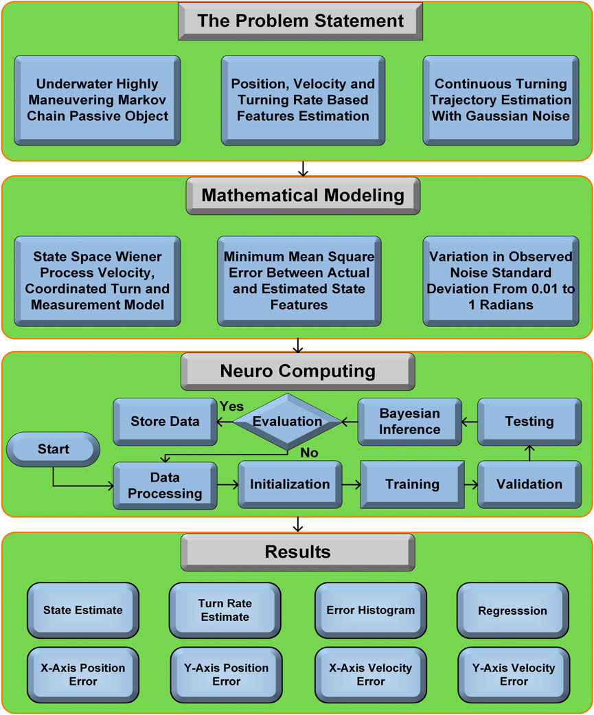
Figure 1. Graphical description of proposed paradigm.

2 System modeling of passive underwater object

In this portion of the study, the modeling of Markov chain moving object is designed using a bilateral state feature estimation approach in angular dimensions. This methodology incorporates the state space-based bearings only tracking (BOT) technique to precisely estimate the state features of a constantly rotating object in a complex and difficult marine atmosphere.In order to gather the collation of passive measurements, a total of eight monitoring bases are strategically positioned at equal intervals. The term passive measurements of the moving object refer to the nonlinear and intricate data obtained by hydrophones. It is assumed that the positions of the observers are known beforehand. The sole approach to get the bearings of the dynamic vehicle by passive acquisition from surveillance units. These bearings are relying on the angular position and placement of each individual sensor module. The proposed state feature estimation structure aims to observe target mobility in the far field zone. This observation is based on the prediction of a consistent turning course, which is tracked through the adoption of nonlinear multi model Kalman filters and neuro computing techniques. Figure 2 illustrates the maneuvering trends of a navigational target and its mechanism for estimating state features. Several systems in real life exhibit dynamic modeling variables. The description of these diverse system variables is unlikely to be addressed by a singular model. In the context of real-time state feature estimating applications, it is probable for the modeling values to experience variations during the estimation phase. These mechanisms are commonly referred to as Markov chains or multi models. In these situations, the whole design could diverge if one particular system model is selected. Consequently, the development of a generic movement model for dynamic object that will regulate numerous system models is critical. Coordinated Turn (CT) and Wiener process velocity (WPV) models are applied in this study to explain the underwater navigation object’s kinematics.

Figure 2

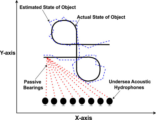
Figure 2. State feature estimation architecture.

2.1 Wiener process velocity (WPV) dynamic modeling

The state vector ${\mathbf{H}}_{\tau }^m$ given in Eq. 1 illustrates the real-time features of a maneuvering object at a given time interval τ, by using bidirectional angular axes to represent its position $\left(\begin{array}{c}{x}_{\tau }\\ y_{\tau }\end{array}\right)$ and velocity $\left(\begin{array}{c}{x}_{\tau }^{\prime }\\ y_{\tau }^{\prime }\end{array}\right)$ as:

${\mathbf{H}}_{\tau }^m=\left[\begin{array}{c}{x}_{\tau }^m\\ y_{\tau }^m\\ {x^{\prime }}_{\tau }^m\\ {y^{\prime }}_{\tau }^m\end{array}\right].(1)$

Concurrently, the state vector at the monitoring unit in angular axes can be represented in Eq. 2 as follows:

${\mathbf{H}}_{\tau }^n=\left[\begin{array}{c}{x}_{\tau }^n\\ y_{\tau }^n\\ {x^{\prime }}_{\tau }^n\\ {y^{\prime }}_{\tau }^n\end{array}\right].(2)$

The state formulation that relates the moving object and the observation station is listed in Eq. 3 below:

${\mathbf{H}}_{\tau }={\mathbf{H}}_{\tau }^m-{\mathbf{H}}_{\tau }^n=\left[\begin{array}{c}{x}_{\tau }\\ y_{\tau }\\ x_{\tau }^{\prime }\\ y_{\tau }^{\prime }\end{array}\right].(3)$

The discrete-time WPV approach is applied to construct the momentum of the maneuvering object under the framework of state-space science. This design is implemented to define the state expression in the following way:

${\mathbf{H}}_{\tau +1}={\mathbf{X}}_{\tau }{\mathbf{H}}_{\tau }+{\alpha }_{\tau }.(4)$

The state model illustrated above defines the dynamic shifting matrix X_τ, which consists of elements ι × ι. The dynamic shifting matrix reflects the response of the WPV model in the context of state-space strategy. It is assumed that process noise α_τ in this model follows a Gaussian spectrum having its mean near zero. The calculation for spread of the dynamic shifting matrix X_τ with respect to the sampling interval is described in Eq. 5 as:

${\mathbf{X}}_{\tau }=\left[\begin{array}{cccc}\hfill 1\hfill & \hfill 0\hfill & \hfill \partial \tau \hfill & \hfill 0\hfill \\ \hfill 0\hfill & \hfill 1\hfill & \hfill 0\hfill & \hfill \partial \tau \hfill \\ \hfill 0\hfill & \hfill 0\hfill & \hfill 1\hfill & \hfill 0\hfill \\ \hfill 0\hfill & \hfill 0\hfill & \hfill 0\hfill & \hfill 1\hfill \end{array}\right],(5)$

while the sampling interval ∂τ is given in Eq. 6 as:

$\partial \tau =\left[\left(\tau +1\right)-\tau \right].(6)$

To ensure precise estimation of state features through the IBRBNC paradigm, it is necessary to transform the state space model outlined in Eq. 4 into discrete time notation. The discrete-time regressive model is adopted because of its potential to achieve more precise assessment of the system’s behavior at time instances τ that are combination of the sampling interval ∂τ. The discrete time state computation has been transformed with its required elements in Eq. 7, resulting in the following form:

${\mathbf{H}}_{\tau +1}=\underset{{\mathbf{X}}_{\tau }}{\underbrace{\left[\begin{array}{cccc}\hfill 1\hfill & \hfill 0\hfill & \hfill \partial \tau \hfill & \hfill 0\hfill \\ \hfill 0\hfill & \hfill 1\hfill & \hfill 0\hfill & \hfill \partial \tau \hfill \\ \hfill 0\hfill & \hfill 0\hfill & \hfill 1\hfill & \hfill 0\hfill \\ \hfill 0\hfill & \hfill 0\hfill & \hfill 0\hfill & \hfill 1\hfill \end{array}\right]}}\underset{{\mathbf{H}}_{\tau }}{\underbrace{\left[\begin{array}{c}\hfill x_{\tau }\hfill \\ \hfill y_{\tau }\hfill \\ \hfill x_{\tau }^{\prime }\hfill \\ \hfill y_{\tau }^{\prime }\hfill \end{array}\right]}}+{\alpha }_{\tau }.(7)$

The process noise α_τ in the Gaussian spectrum is characterized by its covariance ℓ_τ in the following way:

${\alpha }_{\tau }\approx \text{N}(0,{\ell }_{\tau })\text{.}(8)$

In experimental tests, the Gaussian noise variance is typically assigned an integer value of 0.05 in order to generate target trajectory with minimal curves. In contrast,

${\ell }_{\tau }=\text{E}\left[{\alpha }_{\tau }{\alpha }_{\tau }^{\text{T}}\right].(9)$

In order to achieve a discrete-time state expression, it is necessary to distinguish the process Gaussian noise in the WPV mathematical design. It can be adopted to accurately incorporate the model’s parameters over time intervals that are successive integers of ∂τ. Following this methodology, the aforementioned Eq. 9 is modified to represent a covariance matrix as:

${\ell }_{\tau }=\left[\begin{array}{cccc}\hfill 0.3\partial {\tau }^3\hfill & \hfill 0\hfill & \hfill 0.5\partial {\tau }^2\hfill & \hfill 0\hfill \\ \hfill 0\hfill & \hfill 0.3\partial {\tau }^3\hfill & \hfill 0\hfill & \hfill 0.5\partial {\tau }^2\hfill \\ \hfill 0.5\partial {\tau }^2\hfill & \hfill 0\hfill & \hfill \partial \tau \hfill & \hfill 0\hfill \\ \hfill 0\hfill & \hfill 0.5\partial {\tau }^2\hfill & \hfill 0\hfill & \hfill \partial \tau \hfill \end{array}\right]\omega ,(10)$

meanwhile the constant ω in Eq. 10 defines the spectral magnitude of the Gaussian noise.

2.2 Coordinated turn (CT) modeling

The CT design is a commonly used approach for modeling the kinetic properties of a passive target that undergoes continuous axial motion. In this kinetic system modeling, rotation rate is an additional feature in the state vector. Here, the location, velocity, and spin rate of the maneuvering vehicle are represented by its state features vector in angular dimensions. Through the CT model, it can be defined in Eq. 11 as:

${\mathbf{H}}_{\tau }^m=\left[\begin{array}{c}{x}_{\tau }^m\\ y_{\tau }^m\\ {x^{\prime }}_{\tau }^m\\ {y^{\prime }}_{\tau }^m\\ {\omega }_{\tau }^m\end{array}\right].(11)$

As well as, the formulation of the state feature vector at the observation point can be done in Eq. 12 in the following manner:

${\mathbf{H}}_{\tau }^n=\left[\begin{array}{c}{x}_{\tau }^n\\ y_{\tau }^n\\ {x^{\prime }}_{\tau }^n\\ {y^{\prime }}_{\tau }^n\\ {\omega }_{\tau }^n\end{array}\right].(12)$

The corresponding state vector is presented to explain the relationship across the monitoring unit and the maneuvering object as:

${\mathbf{H}}_{\tau }={\mathbf{H}}_{\tau }^m-{\mathbf{H}}_{\tau }^n=\left[\begin{array}{c}{x}_{\tau }\\ y_{\tau }\\ x_{\tau }^{\prime }\\ y_{\tau }^{\prime }\\ {\omega }_{\tau }\end{array}\right].(13)$

The governing state formulation of the CT framework is presented in Eq. 14 as:

${\mathbf{H}}_{\tau +1}={\mathbf{X}}_{\tau }{\mathbf{H}}_{\tau }+\mathrm{\Upsilon }{\alpha }_{\tau }.(14)$

The state formulation in the CT framework closely resembles the configuration described in Eq. 4 of the Wiener process model with a supplementary variable ϒ, that determines the spatial pattern of Gaussian noise α_τ. The discrete-time sequence of state equation for the aforementioned framework is derived from an approach identical to the WPV modeling in Eq. 15 as:

${\mathbf{H}}_{\tau +1}=\underset{{\mathbf{X}}_{\tau }}{\underbrace{\left[\begin{array}{ccccc}\hfill 1\hfill & \hfill 0\hfill & \hfill \frac{\sin \left({\omega }_{\tau }\ell \tau \right)}{{\omega }_{\tau }}\hfill & \hfill \frac{\cos \left({\omega }_{\tau }\ell \tau \right)-1}{{\omega }_{\tau }}\hfill & \hfill 0\hfill \\ \hfill 0\hfill & \hfill 1\hfill & \hfill \frac{1-\cos \left({\omega }_{\tau }\ell \tau \right)}{{\omega }_{\tau }}\hfill & \hfill \frac{\sin \left({\omega }_{\tau }\ell \tau \right)}{{\omega }_{\tau }}\hfill & \hfill 0\hfill \\ \hfill 0\hfill & \hfill 0\hfill & \hfill \cos \left({\omega }_{\tau }\ell \tau \right)\hfill & \hfill -\sin \left({\omega }_{\tau }\ell \tau \right)\hfill & \hfill 0\hfill \\ \hfill 0\hfill & \hfill 0\hfill & \hfill \sin \left({\omega }_{\tau }\ell \tau \right)\hfill & \hfill \cos \left({\omega }_{\tau }\ell \tau \right)\hfill & \hfill 0\hfill \\ \hfill 0\hfill & \hfill 0\hfill & \hfill 0\hfill & \hfill 0\hfill & \hfill 1\hfill \end{array}\right]}}{\mathbf{H}}_{\tau }+\underset{\mathrm{\Upsilon }}{\underbrace{\left[\begin{array}{c}\hfill 0\hfill \\ \hfill 0\hfill \\ \hfill 0\hfill \\ \hfill 0\hfill \\ \hfill 1\hfill \end{array}\right]}}{\alpha }_{\tau }.(15)$

The CT paradigm additionally incorporates Gaussian dynamical noise given in Eq. 16, consisting of a zero-valued mean and a covariance equivalent to that specified in Eq. 8.

${\alpha }_{\tau }\approx \text{N}(0,{\ell }_{\tau })\text{.}(16)$

The computational analysis of the CT model is displayed in matrix format earlier, even though it has nonlinear dynamics. Consequently, the CT system can be formulated by employing Eqs 17-21 as:

$x_{\tau +1}=x_{\tau }+\frac{\sin \left({\omega }_{\tau }\ell \tau \right)}{{\omega }_{\tau }}{x}_{\tau }^{\prime }+\frac{\cos \left({\omega }_{\tau }\ell \tau \right)-\ell \tau }{{\omega }_{\tau }}{y}_{\tau }^{\prime },(17)$

$y_{\tau +1}=y_{\tau }+\frac{1-\cos \left({\omega }_{\tau }\ell \tau \right)}{{\omega }_{\tau }}{x}_{\tau }^{\prime }+\frac{\sin \left({\omega }_{\tau }\ell \tau \right)}{{\omega }_{\tau }}{y}_{\tau }^{\prime },(18)$

$x_{\tau +1}^{\prime }=\cos \left({\omega }_{\tau }\ell \tau \right)x_{\tau }^{\prime }-\sin \left({\omega }_{\tau }\ell \tau \right)y_{\tau }^{\prime },(19)$

$y_{\tau +1}^{\prime }=\sin \left({\omega }_{\tau }\ell \tau \right)x_{\tau }^{\prime }+\cos \left({\omega }_{\tau }\ell \tau \right)y_{\tau }^{\prime },(20)$

${\omega }_{\tau +1}={\omega }_{\tau }+{\alpha }_{\tau }.(21)$

In the context of experiments, when anticipating significant maneuverability of underwater object, the Gaussian dynamical noise covariance for the rotational feature is set at a particular integer value of 0.15.

2.3 Measurement modeling

In state feature estimation mathematical strategy, each WPV and CT framework corresponds to the same measurement modeling that is developed as well, utilizing the concept of state-space approach. The computational representation of the measurement modeling can be termed as:

${\text{Y}}_{\tau +1}=\mathbf{R}\left({\mathbf{H}}_{\tau +1},{\beta }_{\tau +1}\right).(22)$

Throughout the time intervals τ, the simultaneous passive bearings obtained from maneuvering object are compiled in a matrix R (.), which is commonly known as measurement matrix. It integrates complex passive bearings that are produced using the point-slope tangent interaction algebraic technique. The parameter β in the aforementioned measurement formula represents the detected noise at time interval τ, which follows a distinct Gaussian spectrum. The subsequent computation is carried out to develop passive bearings, which are observed acoustically based on the actual movement of the moving object and the placement of monitoring units.

$\mathbf{R}\left({\mathbf{H}}_{\tau +1}\right)=\underset{\text{Passive\hspace{0.17em}Bearings}}{\underbrace{\text{atan}\left[\frac{y_{\tau }-{\mathrm{\Phi }}_y^i}{x_{\tau }-{\mathrm{\Phi }}_x^i}\right]}}.(23)$

The given measurement equation represents the instantaneous motion of the moving object (y_τ, x_τ) through bilateral angular axes. As well as the placement of hearing observers, symbolized as $({\mathrm{\Phi }}_y^i,{\mathrm{\Phi }}_x^i)$, can be seen in this computation. For the monitoring unit i at time interval τ, the measurement framework Y, as specified in Eq. 22, can be formulated in revised form as:

${\text{Y}}_{\tau }^i=\text{atan}\left[\frac{y_{\tau }-{\mathrm{\Phi }}_y^i}{x_{\tau }-{\mathrm{\Phi }}_x^i}\right]+{\beta }_{\tau }^i.(24)$

In the above-mentioned expression, the observed noise ${\beta }_{\tau }^i$ possesses a zero mean. Whereas the calculation of its covariance ℵ_τ is as follows in Eq. 25.

${\beta }_{\tau }^i\cong \mathrm{N}\left(0,{\aleph }_{\tau }\right),(25)$

${\aleph }_{\tau }=\text{diag}({\sigma }_{\text{Y}}^2)\text{.}(26)$

The observed noise standard deviation given in Eq. 26, denoted by the sign σ, is represented in the above equation. It plays an important role in analyzing the performance of state feature estimation methodologies in the context of underwater object navigation. The dynamics of the subaquatic environment are characterized by the unpredictable nature of the observed standard deviation of acoustic noise. Different metrics for the observed noise standard deviation are adopted in our investigation in order to analyze the robustness and accuracy of the neuro computing and traditional Bayesian approaches. By adhering to the prescribed sequence of maneuvers, a synchronized rotational track can be established for the underwater object.

• The dynamic object commences its motion at a position of $\left[\begin{array}{c}{x}_{\tau }\\ y_{\tau }\end{array}\right]=\left[\begin{array}{c}0\\ 0\end{array}\right]$ and maintaining a constant velocity $\left[\begin{array}{c}{x}_{\tau }^{\prime }\\ y_{\tau }^{\prime }\end{array}\right]=\left[\begin{array}{c}1\\ 0\end{array}\right]$ across the x-axis, sets up its moves from the point of origin.

• Following a time interval of 4 s, the object undergoes a right twist having a rotation rate specified as ω_τ = −1.

• After completing a duration of 9 s, the object ceases its rightward rotation and proceeds to move along normal trajectory, maintaining a consistent velocity of 1 unit.

• The aquatic object exhibits leftward movement with a rotational parameter ω_τ = 1, which occurs at the 11 s interval over the entire period.

• Around 16 s, the vehicle discontinues its leftward turn and proceeds to travel straight ahead at a constant velocity for the duration of 4 s.

3 Neuro computing designing

In this portion of the study, a mathematical framework using smart neuro computing is developed for state feature estimation of underwater moving object. The link between Bayesian normalization deep learning, and underwater localization is their mutual reliance on Bayesian theories for the purpose of managing uncertainties. The primary objective of target localization is to estimate the motion features of a dynamic object. In contrast, Bayesian regularization neuro computing is primarily concerned with modeling the ambiguity that arises from neural network variables. The performance of the estimation approach in state feature applications is significantly influenced by the presence of noisy bearings. Therefore, the basic knowledge of complicated noisy bearings or prior information can be employed for the purpose of modeling IBRBNC in order to obtain the ideal performance of state features.

3.1 Intelligent Bayesian regularization backpropagation neuro computing (IBRBNC)

The IBRBNC is a particular form of neural network model that implements Bayesian concept to make its training operation smoother. The basic objective of Bayesian regularization is to establish a statistical structure for representing the unpredictability associated with the key variables of a network, namely, the weights and biases.

3.1.1 Mathematical modeling of IBRBNC

The IBRBNC framework employs Bayesian approaches, namely, weight priors and posterior variations, in order to incorporate regularization into the system. Regularization plays a crucial role in mitigating overfitting, hence enhancing the effectiveness of IBRBNC in scenarios such as limited access to data or noisy training samples. Taking advantage of the Bayesian approach in the context of IBRBNC enables better management of noisy data. The ability to distinguish actual features from erratic noise enhances the overall robustness of the algorithm. IBRBNC possesses the ability to effectively adjust to different degrees of complexity in the network. The proposed deep learning framework successfully integrates historical information in order to forecast the future outcomes of state features associated with submerged passive navigating object. Within the nonlinear environment of the IBRBNC paradigm, external input and consequent output are employed to forecast the future trends of state features. In this regard, IBRBNC adopts an extremely efficient multi-layer design consisting of an input layer, an embedded layer, a hold layer, and an outcome layer, as depicted in Figure 3. In this particular configuration, the measurement function Y(τ) given in Eq. 24 is applied to the IBRBNC network as input to create estimations regarding the passive object state vector H(τ) given in Eq. 13.

Figure 3

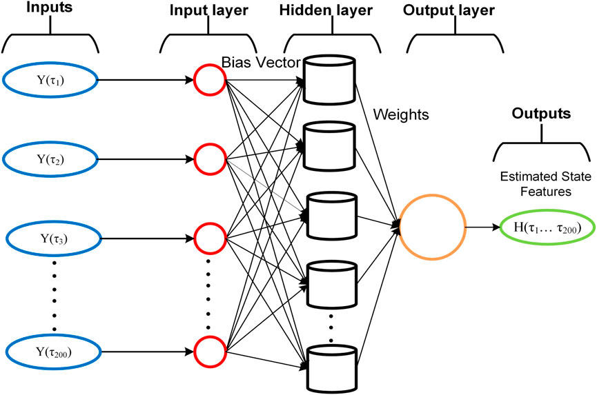
Figure 3. Architecture of Bayesian regularization neural network.

The most difficult aspect of applying the Bayesian regularization approach is determining the appropriate setting for the desired function coefficients. The Bayesian theory implemented in neural systems is founded upon the likelihood analysis of variables inside the network. In comparison with the standard procedure for network training, which selects the best combination of weights by reducing divergence, the Bayesian strategy incorporates a probabilistic spectrum of network weights. Consequently, the outputs of the network can be characterized by spectrum of likelihoods. Let us suppose a Bayesian neuro computing architecture that uses a learning data set S, which comprises z numbers of input and target matrix pairs. These pairings are used to train the neural model.

$\text{S\hspace{0.17em}}=\left\{\left({\text{Y}}_1,{\mathbf{H}}_1\right),\left({\text{Y}}_2,{\mathbf{H}}_2\right),\dots ,\left({\text{Y}}_z,{\mathbf{H}}_z\right)\right\}.(27)$

During the training stage, it is preferred to determine a standard evaluation metric for calculating the difference among actual and estimated data. The aforementioned metric can be mathematically represented in the following manner:

${\text{A\hspace{0.17em}}=\text{\hspace{0.17em}E}}_{\text{S}}\left(\text{S}|e\text{,\hspace{0.17em}F}\right)=\frac{1}{\mathbb{C}}{\displaystyle \sum _{j=1}^{\mathbb{C}}}{\left({\widehat{\mathbf{H}}}_j-{\mathbf{H}}_j\right)}^2.(28)$

In Eq. 28, E_S represents the average sum of squares of the model loss, it is also a measure for prior terminating, which is employed in several computational methods as a means to prevent excessive fitting. S denotes the learning data set, which consists of input-target combos, as defined in Eq. 27. The F is neural network layout, which is characterized by its configuration, that includes the quantity of layers, the size of elements inside each layer, and the particular trigger function employed by each element. In an IBRBNC model, the process of normalization includes a supplementary parameter in the desired function. This parameter is used to minimize the presence of massive weights, which can potentially result in more consistent mapping. In the present scenario, it is appropriate to use the gradient-based optimization method in order to effectively minimize the objective function.

$\text{A\hspace{0.17em}}=\eta {\text{E}}_{\text{S}}\left(\text{S}|e\text{,\hspace{0.17em}F}\right)+\kappa {\text{E}}_{\mathit{weight}}\left(e|\text{F}\right).(29)$

The term E_weight (e|F) in Eq. 29 represents the sum of squares of model weights, described in Eq. 30 as:

${\text{E}}_{\mathit{weight}}=\frac{1}{\mathbb{C}}{\displaystyle \sum _{j=1}^{\mathbb{C}}}{e}_j^2.(30)$

A pair of hyperparameters η and κ are needed to be computed as coefficients of the desired function. The closing term denoted as κE_weight (e|F), is commonly referred to as weight decay, while κ is alternatively recognized as the decay ratio. If the value of κ is significantly smaller than η, the neuro computing network will decrease mistakes. When κ is significantly larger than η, the training process will prioritize reducing the size of the weights, even if it leads to an increase in network mistakes. As a result, the network’s outcome will become more convenient. Once the data has been acquired, assuming Gaussian noise in the target samples, the subsequent spectrum of the weights in the neural network can be adjusted by applying Bayes’ rule.

$\text{P}\left(e|\text{S,}\kappa \text{,}\eta \text{,F}\right)=\frac{\text{P}\left(\text{S}|e,\eta ,\text{F}\right).\text{P}\left(e|\kappa ,\text{F}\right)}{\text{P}\left(\text{S}|\kappa ,\eta ,\text{F}\right)}.(31)$

Hence, Bayesian regularization incorporates a likelihood spectrum of network weights, defining the system architecture as a stochastic platform. In Eq. 31, the variable S represents the training sample, whereas the prior allocation of weights is formalized in Eq. 32 as:

$\text{P}\left(e|\kappa \text{,\hspace{0.17em}F}\right)={\left(\frac{\kappa }{2\pi }\right)}^{u/2}\exp \left\{-\frac{\kappa }{2}e{e}^{\prime }\right\}.(32)$

The neural network layer design is denoted as F, while the vector e represents the weights associated with the architecture. The term $\text{P}\left(e|\kappa \text{,\hspace{0.17em}F}\right)$ denotes understanding of weights prior to the acquisition of any dataset. The probability function, indicated as $\text{P}\left(\text{S}|e,\eta ,\text{F}\right)$, represents the likelihood of the happening of dataset pairs, specifically in relation to the design weights. Within the constraints of this Bayesian scheme, the most desirable weights are those that increase the subsequent likelihood, denoted as $\text{P}\left(e|\text{S,}\kappa \text{,}\eta \text{,F}\right)$. The process of improving the subsequent probability of weights e can be regarded as similar to the process of reducing the normalized desired function A = ηE_S + κE_weight. Let us assume the combined posterior density in Eq. 33 as:

$\text{P}\left(\kappa \text{,}\eta |\text{S,\hspace{0.17em}F}\right)=\frac{\text{P}\left(\text{S}|\kappa ,\eta ,\text{F}\right).\text{P}\left(\kappa ,\eta |\text{F}\right)}{\text{P}\left(\text{S}|F\right)}.(33)$

It can be observed in Eq. 34 as:

$\text{P}\left(\text{S}|\kappa ,\eta ,\text{F}\right)=\frac{\text{P}\left(\text{S}|e,\eta ,\text{F}\right)\text{P}\left(e|\kappa \text{,}\text{F}\right)}{\text{P}\left(e|\text{S,\hspace{0.17em}}\kappa ,\eta ,\text{F}\right)},(34)$

$\text{P}\left(\text{S}|\kappa ,\eta ,\text{F}\right)=\frac{{\nabla }_{\text{A}}\left(\kappa ,\eta \right)}{{\left(\pi /\eta \right)}^{v/2}{\left(\pi /\kappa \right)}^{u/2}}.(35)$

Whereas v represents the sum of the findings and u indicates the entire set of network coefficients. The Laplace approximation, represented in Eq. 35, yields the subsequent mathematical expression:

${\nabla }_{\text{A}}\left(\kappa ,\eta \right)\propto \frac{1}{\sqrt{\left|{\mathbf{X}}^{\mathit{BAP}}\right|}}\exp \left(-\text{A}\left(e^{\mathit{BAP}}\right)\right).(36)$

The Hessian matrix of the desired function is denoted by X^BAP in Eq. 36, while BAP is an acronym that refers to best a posteriori. The Hessian matrix may be estimated as:

$\mathbf{X}=\text{JJ’}\text{.}(37)$

Here letter J in Eq. 37 represents the Jacobian matrix, which comprises the partial derivatives of the network failures relative to the network variables. While J can be defined in Eq. 38 as:

$\text{J\hspace{0.17em}}=\left[\begin{array}{cccc}\hfill \frac{\partial {\mu }_1\left(e\right)}{\partial e_1}\hfill & \hfill \frac{\partial {\mu }_1\left(e\right)}{\partial e_2}\hfill & \hfill \cdots \hfill & \hfill \frac{\partial {\mu }_1\left(e\right)}{\partial e_{\text{q}}}\hfill \\ \hfill \frac{\partial {\mu }_2\left(e\right)}{\partial e_1}\hfill & \hfill \frac{\partial {\mu }_2\left(e\right)}{\partial e_2}\hfill & \hfill \cdots \hfill & \hfill \frac{\partial {\mu }_2\left(e\right)}{\partial e_{\text{q}}}\hfill \\ \hfill ⋮\hfill & \hfill ⋮\hfill & \hfill \ddots \hfill & \hfill ⋮\hfill \\ \hfill \frac{\partial {\mu }_{\text{Q}}\left(e\right)}{\partial e_1}\hfill & \hfill \frac{\partial {\mu }_{\text{Q}}\left(e\right)}{\partial e_2}\hfill & \hfill \cdots \hfill & \hfill \frac{\partial {\mu }_{\text{Q}}\left(e\right)}{\partial e_{\text{q}}}\hfill \end{array}\right].(38)$

The selection between the Gauss-Newton (GN) estimation approach and the Hessian matrix is an essential factor when implementing the Levenberg-Marquardt (LM) training method for the optimization of the objective function A. In the context of the LM algorithm, the variables at the rth loop are modified in Eq. 39 as:

$e^{r+1}=e^r-\left[\frac{1}{{\text{J}}^{\text{T}}\text{J}+\epsilon I}\right]{\text{J}}^{\text{T}}\mu \text{.}(39)$

Whereas ɛ represents the Levenberg attenuation coefficient. The variable ɛ can be adjusted with every repetition, which improves the process of optimization. It is widely adopted as an alternative to the GN approach for the purpose of identifying the lowest value of the given function.

3.1.2 Working principle of IBRBNC

The operation and work flow of the IBRBNC can be summarized as follows: Begin.

1. Preliminary processing of data:

• Regularization of given data

• Dividing data into training set, validation set, and test set

2. Initialization phase:

• Layout of the network configured by choosing the number of neurons, layers and delays

• Specify the weights and biases for the pre dispersion values

3. Training:

• Regarding every training instance:

• Feed forward cycle:

• Calculate the system outcome

• Determine Probability:

• Use training data alongside the network outcome to figure out the probability value

• Figure out preceding:

• Using the previous dispersion variables, compute the preceding value

• Calculate the posterior:

• Use Bayes’ formula to figure out the posterior dispersion

• Regularization:

• Apply regularization value to adjust weights

• Backpropagation:

• Determine weights and biases variations

• Modify variables:

• Through gradient descent optimization approach, improve weights and biases

4. Validation:

• Measure effectiveness of the network by validation sample

• Examine for overestimation or convergence

• If required, modify the normalization constants

5. Testing:

• Utilize the test sample to generate estimations using the trained IBRBNC

6. Possible Inference:

• If complete Bayesian inference is needed, then:

• To estimate the subsequent probability over network’s variables, use Bayesian inference approach (Markov Chain Monte Carlo)

7. Evaluation:

• Evaluate the IBRBNC success using test sample

• Calculate the estimation instability, if necessary

Finish.

The overall operational framework of the IBRBNC is depicted in Figure 4.

Figure 4

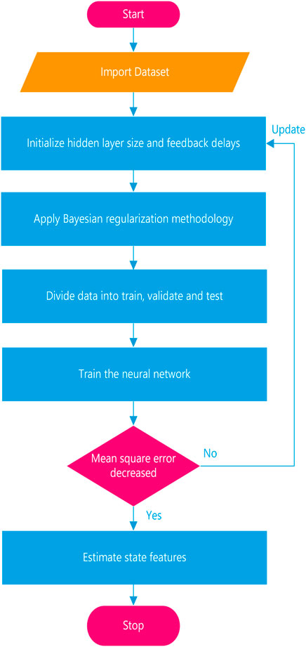
Figure 4. Flow chart of the IBRBNC paradigm.

The data that is fed to the IBRBNC design, as shown in Figure 5, consists of the passive bearings Y(τ) acquired from eight acoustical hydrophones. The bearings information provided to the IBRBNC network for the purpose of computing the estimated state vector H(τ) of five state features. This vector is also depicted as the outcome of the neural system. The layout of the IBRBNC model consists of three layers, namely, the input layer, hidden layer, and output layer, as illustrated in Figure 5.

Figure 5

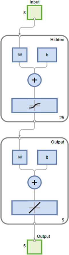
Figure 5. Neural network toolbox flow diagram for IBRBNC.

Eq. 13 in CT model represents real state vector that consists of five different features: the position along the x-axis, the position along the y-axis, the velocity along the x-axis, the velocity along the y-axis, and a variable related to turning around. The state vector is incorporated into the measurement framework, as depicted in Eq. 22, in order to calculate passive bearings. The passive bearings obtained from multiple acoustic hydrophones are processed as input for the IBRBNC infrastructure. This input serves to estimate the state vector, which consists of five state features. In experiments, a concealed layer comprising 25 neurons is deployed, wherein the triggering of these neurons is assisted by a sigmoid function. The process of training weights is achieved by employing Bayesian regularization-based training methodology, which incorporates the backpropagation through time (BPTT) mechanism. Similarly, the application of the epoch format is carried out throughout the training stage of the neuro computing paradigm. Through the process of simulation experiments using the IBRBNC paradigm, the data is divided into three parts. Specifically, 70% of the complete dataset is assigned to the training stage, while the remaining 30% is evenly distributed among the testing and validating processes. This allocation allows the evaluation of the outputs generated by the neuro computing network.

3.2 Assessment metrics

The evaluation standard for the approach of deep neuro computing refers to the development of a reduced MSE between the actual and forecasted state features of maneuvering object at every single moment τ. This research provides an investigation of the accuracy and robustness demonstrated by the neuro computing paradigm. Consequently, the MSE metric to analyze the performance of IBRBNC, IMMEKF, and IMMUKF is generated independently during every Monte Carlo simulation as:

$\text{Error}\left(\tau \right)=\frac{1}{j}{\displaystyle \sum _{\tau =1}^j}{‖{\mathbf{H}}_{\tau }^{\mathit{Real}}-{\mathbf{H}}_{\tau }^{\mathit{Estimates}}‖}^2.(40)$

The moving object’s real state features in the described error Eq. 40 are represented by the variable ${\mathbf{H}}_{\tau }^{\mathit{Real}}$. In contrast, ${\mathbf{H}}_{\tau }^{\mathit{Estimates}}$ expresses the predicted state features of the object, which are computed using IBRBNC and Bayesian filtering methodologies. The entire quantity of data samples is represented by the variable j, which has an amount of 200 in trials. Additionally, the initial data sample is given by τ = 1. The calculation of deviations in state features for the bending trajectory is performed on every sample of time.

4 Discussion on simulation results

This segment of the paper presents a brief discussion of the simulation outcomes for the proposed deep learning approach based on IBRBNC. The findings comprise on estimates of state features in real-time, errors in object’s position on the x and y-axes, divergence in object’s velocity on the x and y-axes, estimates of its rotation, a histogram of inaccuracies and analysis on regression. Five particular circumstances are simulated, and the assessment metrics is standard deviation of observed Gaussian noise. The level of this metrics is consistently adjusted within a range of 0.01–1 radian. The observed noise demonstrates a complicated maritime atmosphere when magnitude reaches its maximum, which is 1 radian. The optimal environment, on the other hand, is characterized by the lowest value, specifically 0.01 radians. In experiments, it is crucial to accurately manipulate the numerical factors of the state estimation model for better state feature estimation and to obtain the required outcomes. Table 1 presents the optimal setting of the parameters used in state estimation modeling.

Table 1

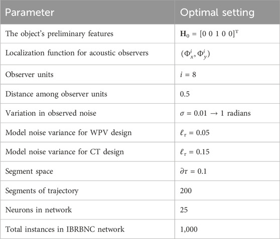
Table 1. Establishing various parameters of state features estimation model.

4.1 Assessment of navigating object state features with different levels of observed noise standard deviations

This part provides a comprehensive analysis of the simulation findings and a detailed discussion on the real-time estimates of state features for a dynamic object. The study implements Bayesian estimation approaches, including IMMEKF, IMMUKF, and IBRBNC. This investigation is aimed to compare the predictability and resolution efficiency of the IBRBNC strategy with IMM Kalman filters. The investigation mainly emphasizes on five distinct levels of recorded noise standard deviation. The statistics from Figures 6–15 exhibit diverse findings obtained from the filtering algorithms and IBRBNC paradigm. These findings represent state estimates, x-axis position error, y-axis position error, x-axis velocity error, y-axis velocity error, rotation forecasts, error histogram, and regression study. The subsequent parts provide an assessment of five independent scenarios associated with algebraic formulations and simulation outcomes.

Figure 6

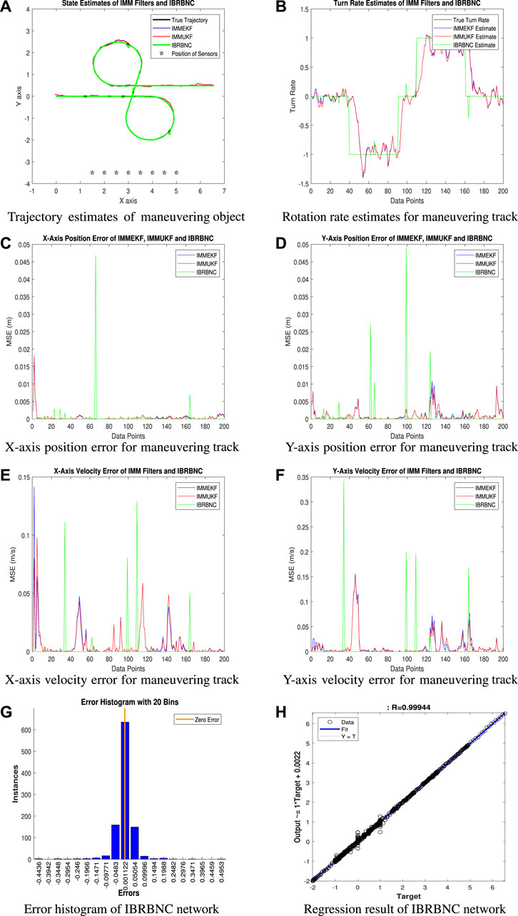
Figure 6. The outcomes of IMMEKF, IMMUKF, and IBRBNC for σ = 0.01 radians.

Figure 7

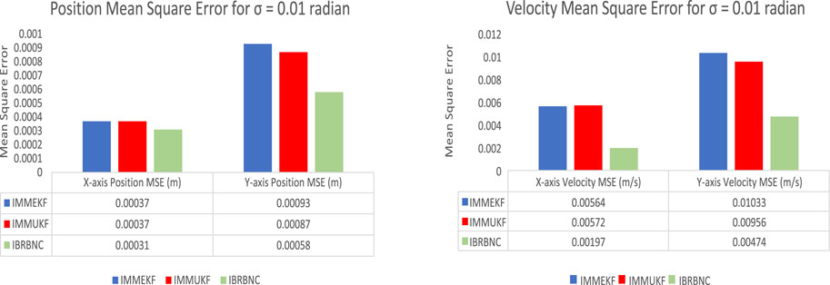
Figure 7. The IMMEKF, IMMUKF, and IBRBNC’s MSEs for estimating bidirectional position and velocity in condition 1.

Figure 8

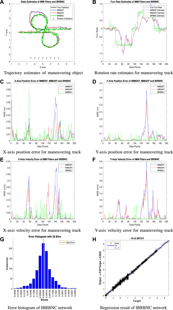
Figure 8. The outcomes of IMMEKF, IMMUKF, and IBRBNC for σ = 0.05 radians.

Figure 9

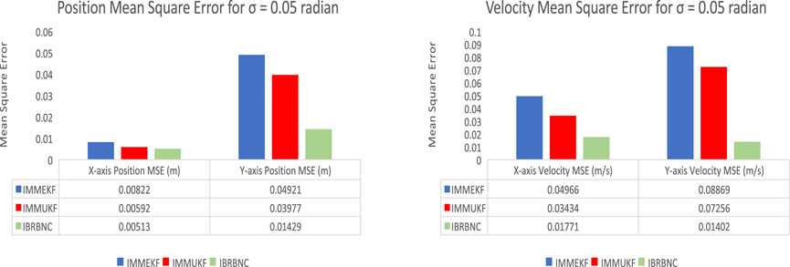
Figure 9. The IMMEKF, IMMUKF, and IBRBNC’s MSEs for estimating bidirectional position and velocity in condition 2.

Figure 10

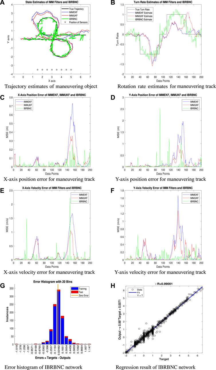
Figure 10. The outcomes of IMMEKF, IMMUKF, and IBRBNC for σ = 0.1 radians.

Figure 11

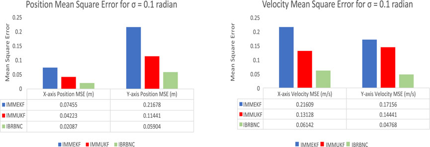
Figure 11. The IMMEKF, IMMUKF, and IBRBNC’s MSEs for estimating bidirectional position and velocity in condition 3.

Figure 12

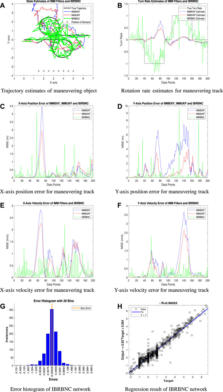
Figure 12. The outcomes of IMMEKF, IMMUKF, and IBRBNC for σ = 0.5 radians.

Figure 13

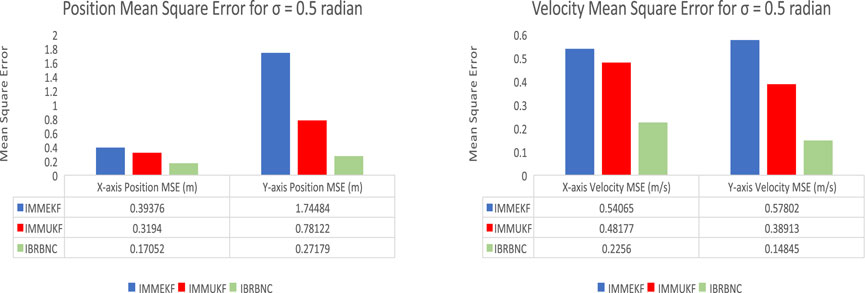
Figure 13. The IMMEKF, IMMUKF, and IBRBNC’s MSEs for estimating bidirectional position and velocity in condition 4.

Figure 14

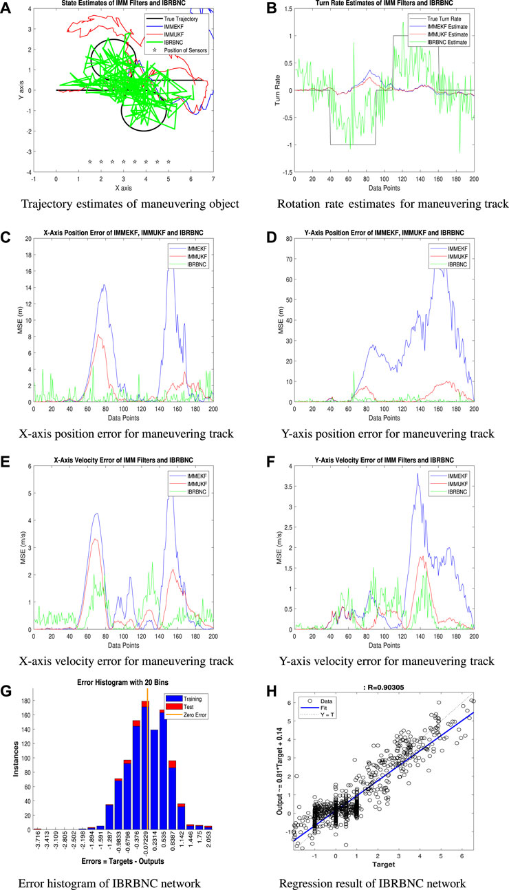
Figure 14. The outcomes of IMMEKF, IMMUKF, and IBRBNC for σ = 1 radian.

Figure 15

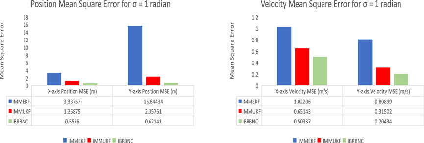
Figure 15. The IMMEKF, IMMUKF, and IBRBNC’s MSEs for estimating bidirectional position and velocity in condition 5.

4.1.1 Condition 1: The observed noise standard deviation σ = 0.01 radians

Gaussian noise ${\beta }_{\tau }^i$ is quantified by 0.01 radians standard deviation in the first condition. This level indicates a nearly ideal oceanic atmosphere with consistently calm circumstances. In this specific instance, the derivation of covariance which contains standard deviation of observed noise is performed in Eq. 41 as:

${\aleph }_{\tau }=\text{diag}({\sigma }_{\text{Y}}^2)\text{.}(41)$

The modeling of the observed noise at particular time interval τ for i sensor is established by employing covariance as:

${\beta }_{\tau }^i\cong \mathrm{N}\left(0,{\aleph }_{\tau }\right).(42)$

The above stated observed noise in Eq. 42 is adding in measurement expression Y as defined for entire passive bearings in Eq. 43 as:

${\text{Y}}_{\tau }^i=\text{atan}\left[\frac{y_{\tau }-{\mathrm{\Phi }}_y^i}{x_{\tau }-{\mathrm{\Phi }}_x^i}\right]+{\beta }_{\tau }^i.(43)$

The IBRBNC paradigm takes the above stated measurement data as its input. The true state vector, as explained in Eq. 44, is used in the measurement model, as shown in Eq. 22, to find out expected state features.

${\mathbf{H}}_{\tau }={\mathbf{H}}_{\tau }^m-{\mathbf{H}}_{\tau }^n=\left[\begin{array}{c}{x}_{\tau }\\ y_{\tau }\\ x_{\tau }^{\prime }\\ y_{\tau }^{\prime }\\ {\omega }_{\tau }\end{array}\right].(44)$

The first scenario demonstrates real-time state approximations, real and observed rotation rates, errors in x-axis and y-axis location, divergences in x-axis and y-axis velocity, an error histogram, and a regression study. All findings compare the true and estimated state features for σ = 0.01 radians observed noise standard deviation. For this scenario, we assume that the marine environment is steady by setting a low integer level for the detected noise.

• In Figure 6A, a comparison is made between the ability of the IBRBNC network and filtering techniques IMMEKF and IMMUKF in the prediction of state features for a navigating object throughout the identification of the turning route. It is worth mentioning that IBRBNC effectively tracks the exact trajectory of the maneuvering object, hence demonstrating its superior precision when compared to the other two approaches.

• Figure 6B depicts the rotational component estimates of the IMMEKF, IMMUKF, and IBRBNC strategies. The better results of the IBRBNC method compared to the IMM predictors are consistently observed throughout the process, as evidenced by the precise estimation of the turning feature for all data points.

• The analysis of the x-axis position inaccuracy is presented in Figure 6C using the mean square approach. Notably, the IBRBNC algorithm exhibits minimal average error when compared to other approaches, except for a single conspicuous spike.

• The simulation results for the y-axis position error of the IMMEKF, IMMUKF, and IBRBNC approaches are presented in Figure 6D. It is obvious that IBRBNC displays occasional spikes while also showcasing a higher average performance when compared to the other approaches. This highlights the effectiveness of IBRBNC in reducing errors in y-axis positioning, demonstrating its technical superiority.

• Figure 6E illustrates the disparity between the true velocity and the estimated velocity along the x-axis, which is measured in MSE context. The deep learning mechanism developed by the IBRBNC demonstrates significant computational efficiency in estimating the velocity along the x-axis. It surpasses the performance of nonlinear Kalman estimators when evaluated using 200 samples. Nevertheless, IBRBNC exhibits small number of spikes that occur during turns of trajectory.

• The simulation results for the y-axis velocity error of the IMMEKF, IMMUKF, and IBRBNC approaches are depicted in Figure 6F. It is worth noting that IBRBNC demonstrates limited sharp climbs while consistently displaying commendable overall performance in comparison to alternative methodologies.

• Figure 6G displays the deviation histogram that represents the discrepancies among the target data ${\mathbf{H}}_{\tau }^{\mathit{Real}}$, and the approximated output ${\mathbf{H}}_{\tau }^{\mathit{Estimates}}$ of the IBRBNC network. The deviation histogram consists of a set of divergence points, encompassing both negative and positive samples. The error values enable to quantify the discrepancy between the input dataset and the computed dataset. In this experiment, the total error of the IBRBNC network is divided into 20 bins, which are graphically depicted as perpendicular segments. The histogram displays an obvious disparity in the central box, as it demonstrates a discrepancy of 0.001122 with samples of 600. This observation implies that several data points display errors that lie within a specific zone. The zero-error line is also located within this box, indicating the neural network’s zero error.

• Figure 6H depicts the regression investigation of the IBRBNC method over the training, validation, and testing phases. The neuro computing platform employs a partitioning strategy to divide the input samples into three distinct subsets: training, validation, and testing. The aforementioned subsets are assigned proportions of 70%, 15%, and 15% respectively. This inspection utilizes probabilistic elements to illustrate the relationship between the findings of state features ${\mathbf{H}}_{\tau }^{\mathit{Estimates}}$ and the corresponding actual state features ${\mathbf{H}}_{\tau }^{\mathit{Real}}$. The regression modeling reveals a substantial level of correlation between the actual and predicted state features. A flat trend is observed in the data sets that reflect the degree of robustness of the IBRBNC paradigm.

Furthermore, the total MSEs for both bidirectional locations and velocities of the underwater object are computed by contrasting the observed values with the predicted values. The results of this condition suggest that the accuracy of the IBRBNC is superior than IMM Kalman filters when considering the responses of position and velocity errors. This illustrates the effectiveness of employing neuro computing for the estimation of state features in underwater maneuvering target scenarios. The graphs presented below illustrate the bidirectional position and velocity errors associated with the IMMEKF, IMMUKF, and IBRBNC techniques.

4.1.2 Condition 2: The observed noise standard deviation σ = 0.05 radians

In condition 2, the standard deviation of observing noise is chosen to be σ = 0.05 radians. The intent of this selection is to deliberately apply a certain amount of observed noise to the computational process. In this specific situation, the calculation of covariance is obtained in Eq. 45 by utilizing the standard deviation of observed noise as:

${\aleph }_{\tau }=\text{diag}({\sigma }_{\text{Y}}^2)\text{.}(45)$

The noise reported for time period τ at hydrophone i belongs to the Gaussian spectrum, with its parameters given by the formerly computed covariance in Eq. 46 as:

${\beta }_{\tau }^i\cong \mathrm{N}\left(0,{\aleph }_{\tau }\right).(46)$

The measurement mechanism of sensor i includes observed noise at every point in time τ as:

${\text{Y}}_{\tau }^i=\text{atan}\left[\frac{y_{\tau }-{\mathrm{\Phi }}_y^i}{x_{\tau }-{\mathrm{\Phi }}_x^i}\right]+{\beta }_{\tau }^i.(47)$

Likewise, the neural paradigm integrates this designed measuring model ${\text{Y}}_{\tau }^i$ given in Eq. 47 as an input. The desired value of IBRBNC is denoted by the subsequent vector of state features given in Eq. 48 as:

${\mathbf{H}}_{\tau }={\mathbf{H}}_{\tau }^m-{\mathbf{H}}_{\tau }^n=\left[\begin{array}{c}{x}_{\tau }\\ y_{\tau }\\ x_{\tau }^{\prime }\\ y_{\tau }^{\prime }\\ {\omega }_{\tau }\end{array}\right].(48)$

The state elements used in the estimation process exploiting the IBRBNC methodology consist of the instantaneous direction of the moving object (x_τ, y_τ), its velocity $(x_{\tau }^{\prime },y_{\tau }^{\prime })$, and its rotation rate ω_τ. The subsequent section showcases the simulation outcomes, encompassing state estimations, rotational approximations, errors in the position of the x and y-axes, errors in the velocity of the x and y-axes, a histogram illustrating divergence, and an analysis of regression for the current condition.

• Figure 8A displays a comparative analysis of all three techniques for state feature estimation by following the turning route of the maneuvering target. It is important to highlight that, in this particular case, the motion estimations and accuracy of IBRBNC are superior to conventional nonlinear filtering approaches.

• The estimated turn rates for the present condition of measurement noise are depicted in Figure 8B. Yet again, the superior performance of the IBRBNC method over standard filtering techniques is achieved for effectively determining the rotation variable.

• The average MSE across actual and predicted x-axis positions of the underwater navigation object is depicted in Figure 8C. Furthermore, this outcome illustrates the degree of accuracy exhibited by the IBRBNC approach in comparison to the IMMEKF and IMMUKF strategies.

• Likewise, y-axis MSE position error of all estimation algorithms is shown in Figure 8D. In this simulation result, IMMEKF and IMMUKF are facing large spikes between 120 and 140 samples. These large spikes are due to their divergence at the left turn of the trajectory. In comparison, IBRBNC is showing the minimum position MSE for all 200 samples of the turning trajectory.

• An analysis of a maneuvering vehicle’s actual and estimated x-axis velocity, computed by IMM filtering techniques and the IBRBNC network, is presented in Figure 8E. The findings show that, in terms of competence, the neuro computing technology executes better than the filtering strategies.

• Figure 8F displays a parallel view of the true and estimated velocity along the y-axis, as computed by all techniques. The results also endorse that the neural learning is estimating better y-axis velocity.

• The error histogram in Figure 8G evaluates the network error between the target dataset ${\mathbf{H}}_{\tau }^{\mathit{Real}}$, and estimated dataset ${\mathbf{H}}_{\tau }^{\mathit{Estimates}}$ of the target’s state features. The bar graph exhibits an inclined bin positioned at its midpoint, which signifies an error of −0.00505. This segment is associated with the input samples and contains an elevation exceeding 200 events. In the given scenario, the zero error is positioned underneath the middle vertical column.

• Figure 8H depicts the IBRBNC computed regression assessment for neural learning. The regression approach demonstrates the usefulness of the IBRBNC framework by illustrating the correlation between the actual intake and the estimated outcome.

The numerical values of average MSEs are also computed to quantify the difference between the actual and predicted bidirectional positions and velocities of the dynamic object in the presence of σ = 0.05 radians noise. The position and velocity errors provide more evidence that potency of the IBRBNC exceeds that of IMM Kalman filters. This demonstrates the efficacy of neural networks in forecasting state characteristics. Figure 9 lists the position and velocity errors derived from IBRBNC and Bayesian Kalman filters.

4.1.3 Condition 3: The observed noise standard deviation σ = 0.1 radians

Under this condition, the observed noise standard deviation increases to σ = 0.1 radians, suggesting that a significant amount of interference has been added in the whole model. Considering standard deviation of 0.1 radians for random detected noise, the variance ℵ at time step τ is computed in Eq. 49 as follows:

${\aleph }_{\tau }=\text{diag}({\sigma }_{\text{Y}}^2)\text{.}(49)$

The mathematical description of the measured noise that is derived from the above covariance for i sensor at time interval τ is given in Eq. 50 as follows:

${\beta }_{\tau }^i\cong \mathrm{N}\left(0,{\aleph }_{\tau }\right).(50)$

The observational model is including the achieved Gaussian measured noise as:

${\text{Y}}_{\tau }^i=\text{atan}\left[\frac{y_{\tau }-{\mathrm{\Phi }}_y^i}{x_{\tau }-{\mathrm{\Phi }}_x^i}\right]+{\beta }_{\tau }^i.(51)$

The above Eq. 51 represents the measurement model Y for hydrophone i at time step τ. This model combines the passive orientations observed by acoustic hydrophones, and correlates them with the white Gaussian distributed measured noise. The data set utilized for deep neuro computing is comprised on the calculations of the measurement model. The neural network’s output consists of state features following Eq. 52, which are presented in state vector as:

${\mathbf{H}}_{\tau }={\mathbf{H}}_{\tau }^m-{\mathbf{H}}_{\tau }^n=\left[\begin{array}{c}{x}_{\tau }\\ y_{\tau }\\ x_{\tau }^{\prime }\\ y_{\tau }^{\prime }\\ {\omega }_{\tau }\end{array}\right].(52)$

The following part provides the simulation results on this value of measured noise in terms of trajectory predictions, turning rate estimates, least bidirectional location errors, divergences in x and y-axes velocities, network failure histogram, and a regression study.

• The state features estimation performance for the synchronized spin track is plotted in Figure 10A for all techniques. It is evident that the deep learning model based on IBRBNC demonstrates superior accuracy when compared to the conventional IMMEKF and IMMUKF methodologies in this particular scenario. The IBRBNC technique demonstrates better capability for precisely determining the dynamics of maneuvering object over bends of the route, in contrast to conventional filters, which face larger hurdles in this regard. This shows the effectiveness of the neural approach.

• Figure 10B illustrates the turn rate predictions based on all methods. Neuro computing demonstrates far better estimation outcomes and achieve turn rates that are close to the actual values, surpassing the capabilities of Kalman filters.

• The plot shown in Figure 10C depicts the real-time mean square positioning inaccuracy along the x-axis for IMM and IBRBNC estimation approaches. IBRBNC demonstrates high precision compared to other techniques in all instances of turning course.

• In Figure 10D, position error along the y-axis is represented for all state feature estimation algorithms. IBRBNC is experiencing some large spikes near 100 data points, while between 120 and 180 samples, the performance of IMM filters is poor. As a whole, the average mean square error of neural learning is better than conventional techniques.

• Figure 10E illustrates the velocity inaccuracy along the x-axis, calculated in meter per second, of the navigation vehicle for every single sample over all methods. All estimation mechanisms are facing decline in accuracy at the intersections of the turning path. Yet, it is obvious that IBRBNC technique surpasses the IMM filters in performance across all sample points.

• Mean square velocity error computed by all estimation algorithms along y-axis of the underwater dynamic object is shown in Figure 10F. In this result, the estimation accuracy of IBRBNC method is steady for all data points while IMM filtering methods are showing large fluctuations, especially at turns of the target trajectory.

• Figure 10G displays a histogram comparing the error of neural learning between target ${\mathbf{H}}_{\tau }^{\mathit{Real}}$, and the expected dynamic features ${\mathbf{H}}_{\tau }^{\mathit{Estimates}}$ of the turning object. The histogram features a centrally positioned upward line, that corresponds to an error value of 0.02482. The maximum value of the vertical bin used for training is nearly 350 points, and the testing samples likewise fall within this limit. The investigation reveals that the zero error is situated inside this upward box, such as an integer of 0.02482.

• Figure 10H depicts the regression conditions that occur throughout the learning process of IBRBNC. The graph illustrates a slight discrepancy between the input and outcome data, which can be indicated by increase in the observed noise.

The current circumstance entails calculating the MSEs for both bidirectional orientations and velocities. The units used for these calculations are meter and meter per second, respectively. The recognition of position and velocity lapses helps to verify the previously described results, providing evidence that the neural system exhibits significantly higher convergence in comparison to multi model filtering methods. The graph presented in Figure 11 illustrates the bidirectional position and velocity inaccuracies obtained through the implementation of the IMMEKF, IMMUKF, and IBRBNC algorithms.

4.1.4 Condition 4: The observed noise standard deviation σ = 0.5 radians

The standard deviation of noise in passive observations is increased to σ = 0.5 radians in this case, so adding a large level of Gaussian disturbance into the state feature estimation mechanism. Here is the formulation of variance in Eq. 53, which includes this numerical value of the standard deviation of the observed noise as:

${\aleph }_{\tau }=\text{diag}({\sigma }_{\text{Y}}^2)\text{.}(53)$

As well as, the calculation of observed Gaussian noise is derived in Eq. 54 from the covariance in the following way:

${\beta }_{\tau }^i\cong \mathrm{N}\left(0,{\aleph }_{\tau }\right).(54)$

The comprehensive framework’s measurement equation incorporates the noise recorded at time step τ for each observer element i in the subsequent form:

${\text{Y}}_{\tau }^i=\text{atan}\left[\frac{y_{\tau }-{\mathrm{\Phi }}_y^i}{x_{\tau }-{\mathrm{\Phi }}_x^i}\right]+{\beta }_{\tau }^i.(55)$

The IBRBNC network is given the complete measurement model formulation ${\text{Y}}_{\tau }^i$ in Eq. 55 as input dataset. It includes passive bearings and observed noise. The desired statistics correspond to the actual state vector, as depicted in Eq. 56 here:

${\mathbf{H}}_{\tau }={\mathbf{H}}_{\tau }^m-{\mathbf{H}}_{\tau }^n=\left[\begin{array}{c}{x}_{\tau }\\ y_{\tau }\\ x_{\tau }^{\prime }\\ y_{\tau }^{\prime }\\ {\omega }_{\tau }\end{array}\right].(56)$

The bidirectional positions, velocities, and rotations of underwater moving vehicle are computed here in real-time for the precise curving path. The motion features are obtained via IMM Kalman filters and neural network leveraging IBRBNC. The actual state vector is employed to estimate the desired characteristics of the underwater object. The diagrams below illustrate simulation findings for path predictions, rotational approximations, oversights in x and y-axes locations, errors in x and y-axes velocities, a histogram of deviations, and the description of regression.

• The state feature estimation capability of Bayesian filtering and IBRBNC schemes is shown in Figure 12A, assuming a lot of observation distortion. It is notable that each of these strategies faces difficulties when attempting to precisely identify the real route of the target. Nevertheless, despite the existence of an adverse underwater environment, it can be seen that the IBRBNC algorithm demonstrates a greater level of coherence with the true trajectory in comparison to the other methodologies under consideration.

• The rotation rate estimates in this specific scenario are illustrated in Figure 12B. This demonstrates that neural computation has more effective predictive approach than IMM filtering methods.

• The schematic diagram denoted as 12c depicts the MSE among the actual and estimated x-axis coordinates of the moving target. The results show that filtration techniques have a notable margin of error, whereas the IBRBNC method provides better convergence with less average positional inaccuracy.

• The underwater object’s mean square position error along the y-axis is represented in Figure 12D. This outcome shows that all algorithms are providing large peaks of error due to enhance noise level. In comparison, the y-axis position prediction performance of neural computing is better than other two techniques.

• Figure 12E exhibits the discrepancy in velocity inaccuracy along the x-axis, which arises from different methods, thereby confirming the efficacy of the neural network model.

• The y-axis mean square velocity errors for all samples of turning trajectory are shown in Figure 12F. In this finding, the estimation accuracy of IBRBNC is far better than conventional techniques for all data points.

• A divergence histogram shown in Figure 12G presents the frequency of deviations across the target information ${\mathbf{H}}_{\tau }^{\mathit{Real}}$, and the estimated target’s motion characteristics ${\mathbf{H}}_{\tau }^{\mathit{Estimates}}$. The difference of −0.00828 is observed in the massive frame positioned in the middle of the chart. In the histogram, the zero-error line is situated beneath the vertical bar with a numerical value of −0.00828.

• The result of the regression in the given case is depicted in Figure 12H, which suggests a substantial gap between the input dataset and the expected outcome. The gap can be identified as an increase in the standard deviation of the observed noise.

To assess the difference between the actual and predicted bidirectional velocity and location of the moving vehicle, the MSE is derived here. The numerical position and velocity divergences strengthen the prior outcomes that IBRBNC demonstrates superior efficiency in comparison to Kalman filters. The position and velocity fluctuations, as computed with the IMMEKF, IMMUKF, and IBRBNC techniques, are depicted in Figure 13.

4.1.5 Condition 5: The observed noise standard deviation σ = 1 radian

In the concluding scenario of this research, a maximum magnitude of σ = 1 radian is chosen to depict an environment that contains an extreme amount of turbulence. Furthermore, the measurement framework with a significant level of noise is employed in the state feature estimation mechanism. The maximum amount of σ relates to the term of covariance ℵ_τ, given in Eq. 57 as:

${\aleph }_{\tau }=\text{diag}({\sigma }_{\text{Y}}^2)\text{.}(57)$

The mathematical modeling of Gaussian distributed observed noise ${\beta }_{\tau }^i$ for sensor i takes place at time τ through the covariance ℵ_τ in Eq. 58 as:

${\beta }_{\tau }^i\cong \mathrm{N}\left(0,{\aleph }_{\tau }\right).(58)$

The measurement formulation in Eq. 59 reflects the presence of excessive amount of distinct white Gaussian observation noise as:

${\text{Y}}_{\tau }^i=\text{atan}\left[\frac{y_{\tau }-{\mathrm{\Phi }}_y^i}{x_{\tau }-{\mathrm{\Phi }}_x^i}\right]+{\beta }_{\tau }^i.(59)$

The input set of data denoted as ${\text{Y}}_{\tau }^i$ for the IBRBNC network, comprises of passive measurements incorporating the highest level of noise. The output of the neuro computing is represented by the state vector, as indicated in Eq. 60 here:

${\mathbf{H}}_{\tau }={\mathbf{H}}_{\tau }^m-{\mathbf{H}}_{\tau }^n=\left[\begin{array}{c}{x}_{\tau }\\ y_{\tau }\\ x_{\tau }^{\prime }\\ y_{\tau }^{\prime }\\ {\omega }_{\tau }\end{array}\right].(60)$

The IBRBNC system combines observations and dynamic functions in a particular order to precisely calculate the output dataset, which includes the estimated vector of state features. The presented information in the below part includes path tracking, rotation predicts, bidirectional locations and velocities discrepancies, error bar chart, and regression approach.

• Figure 14A shows the turning trajectory estimates of IMMEKF, IMMUKF, and IBRBNC algorithms in this specific scenario. The existence of considerable noise in the underwater environment is the reason for the dispersion of route tracking findings among all approaches. Accurately determining the exact path of object presents considerable difficulties across all computational methods. Nevertheless, in this complex circumstance, the intelligent technology referred to as IBRBNC has superior accuracy in forecasting turning path in contrast to conventional methodologies.

• In this high noise level condition, Figure 14B demonstrates the investigation of rotation rate estimations, where the rotation feature is more precisely approximated with IBRBNC.

• Figure 14C displays the MSE representing the average disparity among the actual and anticipated x-axis coordinates of the underwater moving vehicle. The findings conclusively indicate that the IBRBNC paradigm reveals a significantly smaller x-axis position error in comparison to the IMMEKF and IMMUKF techniques.

• In Figures 14A, D comprehensive comparison between IBRBNC and IMM Kalman filters is done for the estimation of y-axis mean position error. In this comparative analysis, neuro computing is showing far better convergence rate and completely dominating IMM filters for all data points of the turning trajectory.

• Figure 14E illustrates the results of the x-axis velocity deviation for all methods. It shows that IBRBNC occasionally has spikes, whereas as a whole it performs better than IMM filtering methods.

• Y-axis velocity error analysis is done in Figure 14F for all applied techniques. In this finding, IBRBNC is showing far better performance in the start and end of the trajectory while experiencing some difficulties in the middle phase of the target’s trajectory. In contrast, the performance of IMM filters is getting worse after 120 data points in the trajectory. Again, IBRBNC is surpassing conventional techniques in this analysis too.

• Figure 14G demonstrates the investigation of neural network by executing the error statistic spectrum. This investigation involves the specific target dataset ${\mathbf{H}}_{\tau }^{\mathit{Real}}$, along with the estimated output dataset ${\mathbf{H}}_{\tau }^{\mathit{Estimates}}$. A disparity of −0.07229 has been identified in an upward box with a training dataset altitude near 170 steps, whereas the testing dataset has heights within the range of 170–180 steps. In this specific situation, the zero-divergence score is located beneath the vertical box, whose center point is −0.07229.

• Figure 14H displays the regression graph of the IBRBNC system, which demonstrates a statistical association between the input dataset and the intended outcome in this condition. The regression evaluation shows a significant difference among the input values and the expected output, which is due to the huge amount of uniformly dispersed noise in the state feature computation architecture.

The average MSEs for the bidirectional location and velocity of the maneuvering vehicle are also numerically calculated in meter and meter per second correspondingly, within this cluttered surrounding. These are determined through contrasting the actual values of the state features with their respective approximate values. The results of the bidirectional location and velocity deviations confirm the prior findings that IBRBNC demonstrates significantly greater precision than Kalman filters, particularly in extremely noisy underwater environments. Figure 15 displays a collection of bidirectional position and velocity mean square errors that have been calculated using the IMMEKF, IMMUKF, and IBRBNC techniques.

The statistics compiled from various conditions indicate that when the standard deviation of observed noise σ is high, all state feature estimation methods encounter difficulties in accurately monitoring the true state of navigational target in marine environment. After doing a thorough comparison of multiple approaches, it is obvious that deep learning using IBRBNC surpasses other strategies in terms of performance. This exceptional results of IBRBNC highlights its capacity to effectively forecast nonlinear real-time state features in underwater problems.

5 Conclusion

The study introduces the ability of deep learning, specifically exploiting the robust IBRBNC paradigm, to accurately estimate state features in real-time for a Markov chain undersea object using just bearing information. The investigation aims to accurately estimate the instantaneous motion features of a kinematic turning target within a two-dimensional x-y coordinate framework at each time instant. The analysis begins by using a mathematical BOT approach to create a model for estimating the state space of the target in both the dynamic and measurement frameworks. Subsequently, a neural computing technique based on IBRBNC is presented to predict the state features of the Markov chain passive object. The performance analysis of the IBRBNC network involves an extensive investigation to find the exact trajectory of target movements using rotation estimates, minimum mean square bidirectional location error, real-time path tracking, bidirectional velocity difference, error histogram, and linear regression. The assessment is conducted using a dataset consisting of 200 samples. Further review involves challenging the suggested method to different numerical values of Gaussian distributed observed noise, leading to a better understanding of its resilience. The outcomes of the simulation in the final section highlight the neural network’s higher level of accuracy in comparison to conventional nonlinear multi-model Bayesian filtering techniques such as IMMEKF and IMMUKF. Recognizing the rapid performance decline over all techniques for noisy measurements, highlights the difficult task of obtaining accurate state features in cluttered oceanic situations. This research represents a significant advancement in enhancing the capacity of underwater systems to estimate the features of moving object. Ultimately leading to improved decision-making and safety in aquatic missions. The establishment of the IBRBNC paradigm presents a great opportunity for further progress in underwater state estimation. It enables new possibilities for applications in marine science, defense, and underwater exploration.

Future research endeavors could investigate the use of recurrent and radial base neural techniques to improve the estimate of state features for objects that are highly maneuverable, even when there is non-Gaussian measurement noise. Exploring this field of research has great potential in underwater atmospheres involving single or many targets.

Data availability statement

The original contributions presented in the study are included in the article/supplementary material, further inquiries can be directed to the corresponding author.

Author contributions

WA: Conceptualization, Data curation, Methodology, Software, Visualization, Writing–original draft, Writing–review and editing. MB: Data curation, Formal Analysis, Methodology, Resources, Supervision, Validation, Writing–review and editing. AA: Funding acquisition, Project administration, Resources, Validation, Writing–review and editing. AJ: Formal Analysis, Funding acquisition, Investigation, Project administration, Validation, Writing–review and editing. AM: Funding acquisition, Writing–review and editing. SH: Resources, Software, Supervision, Writing–review and editing.

Funding

The author(s) declare that financial support was received for the research, authorship, and/or publication of this article. This work was supported by the National Defense Science and Industry Bureau Stability Support Fund (Grant No. JSGG20220831103800001).

Acknowledgments

We are grateful to Prof. Qiao Gang from the College of Underwater Acoustic Engineering, Harbin Engineering University, Harbin for his support and assistance.

Conflict of interest

The authors declare that the research was conducted in the absence of any commercial or financial relationships that could be construed as a potential conflict of interest.

Publisher’s note

All claims expressed in this article are solely those of the authors and do not necessarily represent those of their affiliated organizations, or those of the publisher, the editors and the reviewers. Any product that may be evaluated in this article, or claim that may be made by its manufacturer, is not guaranteed or endorsed by the publisher.

References

1. Yuan S, Li Y, Bao F, Xu H, Yang Y, Yan Q, et al. Marine environmental monitoring with unmanned vehicle platforms: present applications and future prospects. Sci Total Environ (2023) 858:159741. doi:10.1016/j.scitotenv.2022.159741

PubMed Abstract | CrossRef Full Text | Google Scholar

2. Luo J, Han Y, Fan L. Underwater acoustic target tracking: a review. Sensors (2018) 18:112. doi:10.3390/s18010112

PubMed Abstract | CrossRef Full Text | Google Scholar

3. Toky A, Singh RP, Das S. Localization schemes for underwater acoustic sensor networks-a review. Comp Sci Rev (2020) 37:100241. doi:10.1016/j.cosrev.2020.100241

CrossRef Full Text | Google Scholar

4. Huy DQ, Sadjoli N, Azam AB, Elhadidi B, Cai Y, Seet G. Object perception in underwater environments: a survey on sensors and sensing methodologies. Ocean Eng (2023) 267:113202. doi:10.1016/j.oceaneng.2022.113202

CrossRef Full Text | Google Scholar

5. Himri K, Ridao P, Gracias N. Underwater object recognition using point-features, bayesian estimation and semantic information. Sensors (2021) 21:1807. doi:10.3390/s21051807

PubMed Abstract | CrossRef Full Text | Google Scholar

6. Sánchez PJB, Papaelias M, Márquez FPG. Autonomous underwater vehicles: instrumentation and measurements. IEEE Instrumentation Meas Mag (2020) 23:105–14. doi:10.1109/mim.2020.9062680

CrossRef Full Text | Google Scholar

7. Aman W, Al-Kuwari S, Muzzammil M, Rahman MMU, Kumar A. Security of underwater and air–water wireless communication: state-of-the-art, challenges and outlook. Ad Hoc Networks (2023) 142:103114. doi:10.1016/j.adhoc.2023.103114

CrossRef Full Text | Google Scholar

8. Yang J, Huo J, Xi M, He J, Li Z, Song HH. A time-saving path planning scheme for autonomous underwater vehicles with complex underwater conditions. IEEE Internet Things J (2022) 10:1001–13. doi:10.1109/jiot.2022.3205685

CrossRef Full Text | Google Scholar

9. Zhang B, Ji D, Liu S, Zhu X, Xu W. Autonomous underwater vehicle navigation: a review. Ocean Eng (2023) 273:113861. doi:10.1016/j.oceaneng.2023.113861

CrossRef Full Text | Google Scholar

10. Menaka D, Gauni S, Manimegalai CT, Kalimuthu K. Challenges and vision of wireless optical and acoustic communication in underwater environment. Int J Commun Syst (2022) 35:e5227. doi:10.1002/dac.5227

CrossRef Full Text | Google Scholar

11. Ali W, Li Y, Chen Z, Raja MAZ, Ahmed N, Chen X. Application of spherical-radial cubature bayesian filtering and smoothing in bearings only passive target tracking. Entropy (2019) 21:1088. doi:10.3390/e21111088

CrossRef Full Text | Google Scholar

12. Khodarahmi M, Maihami V. A review on kalman filter models. Arch Comput Methods Eng (2023) 30:727–47. doi:10.1007/s11831-022-09815-7

CrossRef Full Text | Google Scholar

13. Herrera PA, Marazuela MA, Hofmann T. Parameter estimation and uncertainty analysis in hydrological modeling. Wiley Interdiscip Rev Water (2022) 9:e1569. doi:10.1002/wat2.1569

CrossRef Full Text | Google Scholar

14. Duník J, Biswas SK, Dempster AG, Pany T, Closas P. State estimation methods in navigation: overview and application. IEEE Aerospace Electron Syst Mag (2020) 35:16–31. doi:10.1109/maes.2020.3002001

CrossRef Full Text | Google Scholar

15. Jahan K, Rao SK. Implementation of underwater target tracking techniques for Gaussian and non-Gaussian environments. Comput Electr Eng (2020) 87:106783. doi:10.1016/j.compeleceng.2020.106783

CrossRef Full Text | Google Scholar

16. Tong F, Griffiths T. Hydrodynamics for subsea systems. In: Encyclopedia of ocean engineering. Singapore: Springer (2022). p. 751–7.

CrossRef Full Text | Google Scholar

17. Abbas MT, Jibran MA, Afaq M, Song WC. An adaptive approach to vehicle trajectory prediction using multimodel kalman filter. Trans Emerging Telecommunications Tech (2020) 31:e3734. doi:10.1002/ett.3734

CrossRef Full Text | Google Scholar

18. Ali W, Li Y, Raja MAZ, Ahmed N. Generalized pseudo bayesian algorithms for tracking of multiple model underwater maneuvering target. Appl Acoust (2020) 166:107345. doi:10.1016/j.apacoust.2020.107345

CrossRef Full Text | Google Scholar

19. Qiu J, Xing Z, Zhu C, Lu K, He J, Sun Y, et al. Centralized fusion based on interacting multiple model and adaptive kalman filter for target tracking in underwater acoustic sensor networks. IEEE Access (2019) 7:25948–58. doi:10.1109/access.2019.2899012

CrossRef Full Text | Google Scholar

20. Kumar M, Mondal S. Recent developments on target tracking problems: a review. Ocean Eng (2021) 236:109558. doi:10.1016/j.oceaneng.2021.109558

CrossRef Full Text | Google Scholar

21. Akhtar S, Habibi S. The interacting multiple model smooth variable structure filter for trajectory prediction. IEEE Trans Intell Transportation Syst (2023) 24:9217–39. doi:10.1109/tits.2023.3271295

CrossRef Full Text | Google Scholar

22. Kolat M, Törő O, Bécsi T. Performance evaluation of a maneuver classification algorithm using different motion models in a multi-model framework. Sensors (2022) 22:347. doi:10.3390/s22010347

PubMed Abstract | CrossRef Full Text | Google Scholar

23. Fu Q, Lu K, Sun C. Deep learning aided state estimation for guarded semi-markov switching systems with soft constraints. IEEE Trans Signal Process (2023) 71:3100–16. doi:10.1109/tsp.2023.3274937

CrossRef Full Text | Google Scholar

24. Ali W, Li Y, Raja MAZ, Khan WU, He Y. State estimation of an underwater Markov chain maneuvering target using intelligent computing. Entropy (2021) 23:1124. doi:10.3390/e23091124

PubMed Abstract | CrossRef Full Text | Google Scholar

25. Ji D, Yao X, Li S, Tang Y, Tian Y. Model-free fault diagnosis for autonomous underwater vehicles using sequence convolutional neural network. Ocean Eng (2021) 232:108874. doi:10.1016/j.oceaneng.2021.108874

CrossRef Full Text | Google Scholar

26. Cheng X, Li G, Ellefsen AL, Chen S, Hildre HP, Zhang H. A novel densely connected convolutional neural network for sea-state estimation using ship motion data. IEEE Trans Instrumentation Meas (2020) 69:5984–93. doi:10.1109/tim.2020.2967115

CrossRef Full Text | Google Scholar

27. Zuberi HH, Liu S, Bilal M, Alharbi A, Jaffar A, Mohsan SAH, et al. Deep-neural-network-based receiver design for downlink non-orthogonal multiple-access underwater acoustic communication. J Mar Sci Eng (2023) 11:2184. doi:10.3390/jmse11112184

CrossRef Full Text | Google Scholar

28. Lin C, Cheng Y, Wang X. A convolutional neural network particle filter for uuv target state estimation. IEEE Trans Instrumentation Meas (2022) 71:1–12. doi:10.1109/tim.2022.3169539

CrossRef Full Text | Google Scholar

29. Ali W, Khan WU, Raja MAZ, He Y, Li Y. Design of nonlinear autoregressive exogenous model based intelligence computing for efficient state estimation of underwater passive target. Entropy (2021) 23:550. doi:10.3390/e23050550

PubMed Abstract | CrossRef Full Text | Google Scholar

30. Cerqueira V, Torgo L, Mozetič I. Evaluating time series forecasting models: an empirical study on performance estimation methods. Machine Learn (2020) 109:1997–2028. doi:10.1007/s10994-020-05910-7

CrossRef Full Text | Google Scholar

31. Zhang Y, Li C, Wang H, Wang J, Yang F, Meriaudeau F. Deep learning aided ofdm receiver for underwater acoustic communications. Appl Acoust (2022) 187:108515. doi:10.1016/j.apacoust.2021.108515

CrossRef Full Text | Google Scholar

32. Polson NG, Sokolov V. Bayesian regularization: from tikhonov to horseshoe. Wiley Interdiscip Rev Comput Stat (2019) 11:e1463. doi:10.1002/wics.1463

CrossRef Full Text | Google Scholar

33. Gecili E, Sivaganesan S, Asar O, Clancy JP, Ziady A, Szczesniak RD. Bayesian regularization for a nonstationary Gaussian linear mixed effects model. Stat Med (2022) 41:681–97. doi:10.1002/sim.9279

PubMed Abstract | CrossRef Full Text | Google Scholar

34. Sariev E, Germano G. Bayesian regularized artificial neural networks for the estimation of the probability of default. Quantitative Finance (2020) 20:311–28. doi:10.1080/14697688.2019.1633014

CrossRef Full Text | Google Scholar

35. Abdullah AA, Hassan MM, Mustafa YT. A review on bayesian deep learning in healthcare: applications and challenges. IEEE Access (2022) 10:36538–62. doi:10.1109/access.2022.3163384

CrossRef Full Text | Google Scholar

36. Liu T, Liu Y, Liu J, Wang L, Xu L, Qiu G, et al. A bayesian learning based scheme for online dynamic security assessment and preventive control. IEEE Trans Power Syst (2020) 35:4088–99. doi:10.1109/tpwrs.2020.2983477

CrossRef Full Text | Google Scholar

37. Ng KH, Tatinati S, Khong AW. Grade prediction from multi-valued click-stream traces via bayesian-regularized deep neural networks. IEEE Trans Signal Process (2021) 69:1477–91. doi:10.1109/tsp.2021.3057691

CrossRef Full Text | Google Scholar

38. Zhou C, Zhang J, Liu J, Zhang C, Shi G, Hu J. Bayesian transfer learning for object detection in optical remote sensing images. IEEE Trans Geosci Remote Sensing (2020) 58:7705–19. doi:10.1109/tgrs.2020.2983201

CrossRef Full Text | Google Scholar

39. Ganji A, Minet L, Weichenthal S, Hatzopoulou M. Predicting traffic-related air pollution using feature extraction from built environment images. Environ Sci Tech (2020) 54:10688–99. doi:10.1021/acs.est.0c00412

CrossRef Full Text | Google Scholar

40. Nguyen C, Li X, Blanton S, Li X. Correlated bayesian co-training for virtual metrology. IEEE Trans Semiconductor Manufacturing (2022) 36:28–36. doi:10.1109/tsm.2022.3217350

CrossRef Full Text | Google Scholar

41. Balram D, Lian KY, Sebastian N. Air quality warning system based on a localized pm2. 5 soft sensor using a novel approach of bayesian regularized neural network via forward feature selection. Ecotoxicology Environ Saf (2019) 182:109386. doi:10.1016/j.ecoenv.2019.109386

PubMed Abstract | CrossRef Full Text | Google Scholar

42. Ye L, Jabbar SF, Abdul Zahra MM, Tan ML. Bayesian regularized neural network model development for predicting daily rainfall from sea level pressure data: investigation on solving complex hydrology problem. Complexity (2021) 2021:1–14. doi:10.1155/2021/6631564

CrossRef Full Text | Google Scholar

43. Price MA, McEwen JD, Pratley L, Kitching TD. Sparse bayesian mass-mapping with uncertainties: full sky observations on the celestial sphere. Monthly Notices R Astronomical Soc (2021) 500:5436–52. doi:10.1093/mnras/staa3563

CrossRef Full Text | Google Scholar

44. Hortúa HJ, Volpi R, Marinelli D, Malagò L. Parameter estimation for the cosmic microwave background with bayesian neural networks. Phys Rev D (2020) 102:103509. doi:10.1103/physrevd.102.103509

CrossRef Full Text | Google Scholar

45. Pignat E, Calinon S. Bayesian Gaussian mixture model for robotic policy imitation. IEEE Robotics Automation Lett (2019) 4:4452–8. doi:10.1109/lra.2019.2932610

CrossRef Full Text | Google Scholar

46. Yuan K, Chatzinikolaidis I, Li Z. Bayesian optimization for whole-body control of high-degree-of-freedom robots through reduction of dimensionality. IEEE Robotics Automation Lett (2019) 4:2268–75. doi:10.1109/lra.2019.2901308

CrossRef Full Text | Google Scholar