Innovative stochastic finite difference approach for modelling unsteady non-Newtonian mixed convective fluid flow with variable thermal conductivity and mass diffusivity

A novel stochastic numerical scheme is introduced to solve stochastic differential equations. The development of the scheme is based on two different parts. One part finds the solution for the deterministic equation, and the second part is the numerical approximation for the integral part of the Wiener process term in the stochastic partial differential equation. The scheme’s stability and consistency in the mean square sense are also ensured. Additionally, a respective mathematical model of the boundary layer flow of Casson fluid on a flat and oscillatory plate is formulated. Wiener process terms perturb the model to be studied. This scheme will be solved in contexts including deterministic and stochastic. The influence of different parameters on velocity, temperature, and concentration profiles is demonstrated in various graphical representations. The main objective of this study is to present a reliable numerical approach that surpasses the limitations of traditional numerical methods to analyze non-Newtonian mixed convective fluid flows with varying transport parameters. Our objective is to demonstrate the capabilities of the new stochastic finite difference scheme in enhancing our comprehension of stochastic fluid flow phenomena. This will be achieved by comprehensively examining its mathematical foundations and computer execution. Our objective is to develop a revolutionary method that will serve as a valuable resource for scientists and engineers studying the modeling and understanding of stochastic unstable non-Newtonian mixed convective fluid flow. This method will address the challenges posed by the fluid’s changing thermal conductivity and mass diffusivity.

1 Introduction

As we know, fluid dynamics is central to studying various other disciplines, such as environmental science, engineering, etc. Also, understanding complex real-world problems demands an insight into the specific characteristics of non-Newtonian fluids. They are the fluids that do not follow the linear relation between the shear stress and the velocity gradient. Casson fluids are a family of viscoplastic materials having yield stress, which is used to model the behaviour of many industrial and biological systems.

Several factors of the fluid, such as temperature, mass diffusivity, etc., affect the behaviour of Casson fluids internally and externally. These factors do not allow an easier way of modelling and recreating the movement of Casson fluids. In addition, Casson fluids frequently flow in systems with spatially varying thermal conductivity and mass diffusivity, necessitating the development of computational techniques that can accurately reflect these fluctuations.

Applications in physical chemistry, metrology, biology, oceanography, astrophysics, plasma physics, etc., all highlight the importance of heat transmission. Liquid distillation, heat exchangers, atomic controller refrigeration, and other technological advances rely heavily on heat transmission. In fluid mechanics, researchers have observed that a certain proportion of mechanical energy is converted into thermal or heat energy due to the resistance generated by viscosity between adjacent fluid layers during their motion. We refer to this as a “switch in internal energy.” First, in his essay [1], Brinkman studied the impact of an internal energy change on capillary flow. Using the impacts of internal energy change and heat transport, Jambal et al. [2] established a power law model and estimated the answer using the finite difference approach. The utilization of nanofluids to improve heat transfer has garnered significant interest among academics in recent years due to its extensive applicability in various industries, such as photonics, electronics, energy production, and transportation [3]. In general, metallic fluids tend to exhibit higher thermal conductivity when compared to non-metallic fluids. Hence, it can be observed that the thermal performance of simple fluids is relatively worse when compared to the thermal performance of metallic nano-sized solid particles dispersed in typical fluids. Nanofluids are formed by introducing microstructural particles into ordinary fluids. These particles, typically composed of metals, carbides, carbon nanotubes, or oxides, have dimensions on the nanometer scale [4, 5]. The nanoparticle composition is crucial in hybrid nanofluids, particularly in enhancing distinctive features such as thermal conductivity. Aziz [6] used the shot method to solve the governing equations, demonstrating the impact of viscous dissipation on an energy equation and the effect of altering thickness on momentum equations.

Nanofluids are the subject of many studies because of their superior conduction qualities that can be achieved through various nanofluid compositions [7, 8]. Herein, we list a few studies conducted along these lines. Nasrin and Alim [9] conducted a numerical study of the heat transmission rate for nanofluids containing dual particles.

Furthermore, a method for simulating micro- and nano-scale fluids has been investigated by Nie et al. [10]. In [11], the writers delve into the theoretical framework of hybrid nanofluids’ heat conduction. The effect of hybrid nanofluids on forced convective heat transfer was estimated statistically by Labib et al. [12].

Investigating fluid flow induced by a horizontally translating surface and its impact on thermo-physical characteristics, such as mass diffusivity, thermal conductivity, and viscosity, is a very captivating subject matter for researchers and scholars. Many studies do not account for or assume that a malleable surface’s thermophysical parameters like conductivity, diffusivity, and viscosity are constant. However, the findings of the experiments show that these thermo-physical properties depend on temperature and concentration, especially in the case of a very large temperature differential. As a result, much attention has been focused on how different thermo-physical factors affect surface stretching. The effect of radiation and thermo-physical factors on the flow of a viscous fluid towards a non-uniform permeable medium was explored by Elbarbary et al. [13]. Saleem studied the effects of various fluid properties on viscous fluid flow through a stretchable medium [14].

Hashim et al. [15] proposed the Willaimson fluid model incorporating nanoparticles, where thermophysical parameters were treated as independent variables. Malik et al. [16] investigated how different fluid properties affected the boundary layer flow of a viscous fluid induced by an expanded cylinder. By assuming exponential functions of temperature for both viscosity and thermal conductivity, Mohiuddin et al. [17] can define the behaviour of a viscoelastic fluid. Second-order fluid flow via a mobile medium in the presence of a heat source/sink was studied by Akinbobola et al. [18], who examined the effect of temperature-dependent physical features of the fluid. Muthucumaraswamy [19, 20] solved the constitutive equations for the flow of a viscous fluid across a non-uniform plate using the Laplace method and variable diffusivity. The 1D -diffusion-advection equation was studied by Jia et al. [21] in two different scenarios: (i) when the thermo-physical characteristics are fixed but the flow velocity is not, and (ii) when the flow velocity and the parameters of the fluid are both changeable. The model was solved, and the resulting outcomes for two scenarios were compared.

The thermo-physical parameters that change with temperature and concentration were studied by Li et al. [22] using the finite difference approach to examine their influence on nonlinear transient responses. The effects of temperature and concentration on the transmission of heat and mass in a viscoelastic fluid flow were examined by Qureshi et al. [23]. Researchers in [24] analyzed Maxwell’s fluid flow model for nanoparticles over a heterogeneous medium, considering thermal effects. Near a vertically moving surface, boundary layer flow is due to cooling and heating impulses [25]. The boundary layer flow around an isothermal, free-moving needle was discussed in [26]. [27] examined the heat transfer parameters of forced convection flow over a non-isothermal thin needle. The Boungirono model of nanofluid flow over a rotating needle was analyzed in [28]. Solving the governing equations involved shooting and fourth-order RK methods. The role of heat production and thermal radiation in MHD The effects of an infinite horizontal sheet on the flow of a Casson fluid in two dimensions were studied in [29].

Animasaun [30] examined how vertically uneven surface roughness affected an unstable mixed convection flow. To investigate the flow’s reaction to a chemical reaction and radiation, he applied the shooting method and quadratic interpolation to the model and then solved it. Shah et al. [32] investigated the effect of the Grashof number on the mixed convection flow of different fluids travelling along different surfaces when heat generation was present. In their study, Animasaun et al. [33] looked at how a chemical process, including quartic autocatalysis, might alter the trajectories of various airborne dust particles. Runge-Kutta, shooting, and bvp4c were used to solve the model’s constitutive equations. The influence of nanoparticles’ random mobility in three-dimensional flow was investigated in a recent meta-analysis by Animasaun et al. [34]. They calculated the heat transfer rate due to the Brownian motion of nanoparticles by considering radiation from the surface and local and mass convection. Researchers at [35] examined how alumina nanoparticles behaved in three dimensions when they carried water or were subject to Lorentz force. They looked into how various dimensionless factors affected the velocities involved.

The article [36] delves into heat transfer in Jeffery-Hamel hybrid nanofluid flows involving non-parallel plates. Molybdenum disulfide nanoparticles are suspended in fluids subjected to magnetic fields, heat radiation, and viscous dissipation. The researcher studied the flow of micropolar fluids across a vertical Riga sheet [37]. We look at the nonlinear stretching sheet. A magnetohydrodynamic (MHD) pair stress hybrid nanofluid on a contracting surface is studied in terms of its radiative properties and overall stability [38].

The difficulties in simulating Casson fluids with non-constant thermal and mass diffusivities can be mitigated with the help of stochastic numerical techniques. To capture the inherent stochasticity in real-world systems, these methods add probabilistic features to account for uncertainties and fluctuations in material qualities. Randomness can be due to material contamination, temperature difference or mass concentration change.

In the past, problems with intricate flows were analyzed by finite difference or finite element methods or by the CFD (Computational Fluid Dynamics) simulations to obtain a better viewpoint of fluid dynamics. Although these methods have enhanced our understanding of the subject, they have often failed to reproduce the inherently stochastic behaviours found in numerous real-world systems accurately. The natural uncertainties in several physical processes in fluid flow are due to numerous boundary conditions, material qualities, and environmental effects. If we do not consider these random variables, then the resulting description of the phenomenon may lead to a misleading picture of reality.

In this work, we examine and assess stochastic numerical methodology for modelling of dynamics of the Casson fluid with arbitrary temperature and density gradients for a better view of how uncertainties and fluctuations in material qualities influence the flow of Casson fluid; we will include a stochastic ingredient in the numerical simulations.

Applications in chemical engineering, geophysics, and biomedicine can significantly profit from gaining exact forecasts of the fundamental behaviour of the fluids to optimize the given processes, develop equipment or know the system’s biological behaviour.

We are at the dawn of applying stochastic probability in fluid mechanics; there is a long way to go. The present article goes into this notion. Let’s consider using stochastic predicting in computational fluid mechanics. We will understand mathematical predicting to describe the behaviours of a physical system’s system within which it operates. Computational models need optimization, design, and updating due to external effects like fluctuations in the natural system and internal elements like uncertainty in the model itself.

Numerous scholars are working hard to figure out stochastic partial differential equations and their numerical solutions. Tessitoe [39] made a seminal discovery in this area when he found that linear and infinite-dimensional stochastic differential equations satisfy the same general conditions as the modified solution. The authors of [40] examined the classical form of the stochastic equation under the assumption of homogeneous Dirichlet boundary conditions. The group set out to see if there were any non-trivial positive global solutions and whether or not those solutions were likely to explode in finite time. Researchers in Ref. [41] examined the Holder continuous coefficient obtained with constant coloured noise to study the stochastic partial differential equation (SPDE). Solving a backward double stochastic differential equation (SDE) allows for path-wise uniqueness and deterministic manipulation of the Laplacian. The solution to a system of stochastic differential equations (SDEs) is found by taking weak limits of a sequence of variables. We obtain this sequence by substituting the discrete Laplacian operator for the random variable in the stochastic partial differential equation (SPDE). Altmeyer et al. explained cellular repolarization using a stochastic variant of the Meinhardt equation. The driving noise process has been shown to influence the evolution of solution patterns for stochastic partial differential equations (SPDEs), and such solutions exist [42]. The solution is fully described in the works mentioned above.

Numerical estimation of stochastic partial differential equations (SPDEs) is a formidable challenge. Instead, Gyorgy et al. [43] worked to construct lattice approximations for elliptic stochastic partial differential equations (SPDEs). For white noise on a restricted domain in $R^d$, $d=1,2,3,$ the convergence rate of approximations is calculated. In [44], we look at how to approximate answers to stochastic partial differential equations of the Itô type. The consistency and stability of these approximations with respect to their mean-square error are established by employing explicit and implicit finite difference techniques. The stochastic Fitz-Hugh-Nagumo model was defined, and a numerical solution was given in [45]. This examination shows how well the technique holds up in a Von Neumann environment [46]. investigated the reliability and robustness of the forward Euler method for evaluating stochastic nonlinear advection-diffusion models. In [47], they consider white noise’s spectral power distribution functions and estimate the numerical approximations for the linear, elliptic, and parabolic cases. The approximations of these cases are evaluated using the finite element and difference methods. The relevant literature dealt with the integral approximation techniques, the finite element methods in these contexts, and the weak SPDE formulation.

This research paper proposes a new and novel numerical scheme for solving the problems of unstable non-Newtonian mixed convection flow of fluid with heat and mass transport with the effect of temperature and concentration fluctuations. The proposed methodology combines stochastic methods in a finite difference scheme, which enables the capture of the random behaviour of the fluid flow in the presence of convective flows. We go for stochastic features in our model and versions of operations to have more accurate predictions and to know more new features in the behaviour of these dynamic systems.

In this work, we shall discuss the theoretical foundation of the fluid dynamics of Casson fluids, the effect of varying thermal conductivity and mass diffusivity in the problems, and introduce some stochastic numerical algorithms for solving such complex flow systems.

The primary contribution of this work is the suggestion of a stochastic numerical scheme for the solution of stochastic partial differential equations. Another method exists in the literature for solving stochastic partial differential equations. That scheme is called the Maruyama method and can be used to solve stochastic equations that appear in fluid dynamics with the variation of Wiener process terms. The Euler-Maruyama method extends the more common forward Euler approach for stochastic differential equations. The Matlab commands generate random numbers from a Normal distribution with a mean of zero and a standard deviation that determines the time step size for the Wiener process term in the scheme.

1.1 Novelty of the study

1. This research presents a distinctive approach by integrating the analysis of Casson fluids with stochastic numerical techniques. Although previous studies have been conducted on Casson fluids and stochastic fluid dynamics modelling, the integration of these two fields remains relatively underexplored in current research. This research presents a fresh way to comprehend the behaviour of non-Newtonian fluids in the presence of changing thermal conductivity and mass diffusivity by including stochastic components in the study of Casson fluids.

2. Variable thermal conductivity and mass diffusivity are considered to solve a practical issue. This variability exists greatly, and various industrial and natural systems have a flowing fluid. To understand how such variations alter the flow behaviour of Casson fluid for practical use in various domains such as chemical engineering, geophysics, biology, etc. To understand how such differences will change the flow behaviour of Casson fluid to be used for actual practical use in different domains such as chemical engineering, geophysics, biology, etc.

3. The challenge exists in yield stress and viscoplastic behaviour modelling the Casson fluid. Moreover, it is already intricate in the modeling process since, unlike other endpoints, strangers constant such as thermal conductivity, mass diffusivity, etc., varies, and materials become parameter-prone. This work is a substantial and novel contribution to fluid dynamics since it addresses the problem of modeling and simulating such complex systems.

4. The random numerical techniques are useful in portraying the level of uncertainty and variability of the qualities of the materials. Using random techniques, the problem of the Casson dynamics can be interpreted.

To portray the sense of randomness and variability, the stochastic numerical technique can be used for modelling the yield stress and viscoelasticity local scalar. The singularity of the present work is underlined by integrating random techniques for studying Casson fluid along with thermal conductivity and mass diffusivity.

2 Proposed computational scheme

This contribution’s stochastic numerical approach can be utilized to solve partial differential equations. The scheme is based on two steps. A partial differential equation’s solution can be predicted in the first step, the predictor stage. The second stage is the corrector stage, which finds the partial differential equation’s solution. But these two stages only find the solution for the deterministic model. The scheme for finding the solution of the stochastic differential equation will be proposed later. For proposing a scheme for a deterministic equation, consider the deterministic equation as follows:

$\frac{\partial v}{\partial t}=G\left(v,\frac{\partial v}{\partial x},\frac{\partial v}{\partial y},\frac{{\partial }^{2}v}{\partial y^2}\right)(1)$

Let the first stage of the scheme be expressed as:

${\overline{v}}_{i,j}^{n+1}=v_{i,j}^n+\Delta t{\left.\frac{\partial v}{\partial t}\right|}_{i,j}^n(2)$

Where $\Delta t$ is the time step size.

The second stage of the scheme is expressed as:

$v_{i,j}^{n+1}=\frac{1}{5}\left(4v_{i,j}^n+{\overline{v}}_{i,j}^{n+1}\right)+\Delta t\left\{a{\left(\frac{\partial v}{\partial t}\right)}_{i,j}^n+b{\left(\frac{\partial \overline{v}}{\partial t}\right)}_{i,j}^{n+1}\right\}(3)$

where $a$ and $b$ will be determined later.

Now, substitute Eq. 2 into Eq. 3, which yields.

$v_{i,j}^{n+1}=\frac{1}{5}\left(4v_{i,j}^n+v_{i,j}^n+\Delta t{\left.\frac{\partial v}{\partial t}\right|}_{i,j}^n\right)+\Delta t\left\{a{\left.\frac{\partial v}{\partial t}\right|}_{i,j}^n+b{\left.\frac{\partial v}{\partial t}\right|}_{i,j}^n+b\Delta t{\left.\frac{{\partial }^{2}v}{\partial t^2}\right|}_{i,j}^n\right\}(4)$

Expanding $v_{i,j}^{n+1}$ using Taylor series expansion

$v_{i,j}^{n+1}=v_{i,j}^n+\Delta t{\left.\frac{\partial v}{\partial t}\right|}_{i,j}^n+\frac{{\left(\Delta t\right)}^2}{2}{\left.\frac{{\partial }^{2}v}{\partial t^2}\right|}_{i,j}^n+O\left({\left(\Delta t\right)}^3\right)(5)$

Substituting Eq. 5 into Eq. 4 gives

$v_{i,j}^n+\Delta t{\left.\frac{\partial v}{\partial t}\right|}_{i,j}^n+\frac{{\left(\Delta t\right)}^2}{2}{\left.\frac{{\partial }^{2}v}{\partial t^2}\right|}_{i,j}^n=v_{i,j}^n+\frac{1}{5}\Delta t{\left.\frac{\partial v}{\partial t}\right|}_{i,j}^n+\Delta t\left\{a{\left.\frac{\partial v}{\partial t}\right|}_{i,j}^n+b{\left.\frac{\partial v}{\partial t}\right|}_{i,j}^n+b\Delta t{\left.\frac{{\partial }^{2}v}{\partial t^2}\right|}_{i,j}^n\right\}(6)$

Evaluating the coefficients of ${\left.\frac{\partial v}{\partial t}\right|}_{i,j}^n$ and ${\left.\frac{{\partial }^{2}v}{\partial t^2}\right|}_{i,j}^n$ on both sides of Eq. 6 that yields

$\left.\begin{array}{c}1=\frac{1}{5}+a+b\\ \frac{1}{2}=b\end{array}\right\}(7)$

Solving Equation 7 gives

$a=\frac{3}{10},b=\frac{1}{2}(8)$

Therefore, the time discretization of Eq. 1 is

${\overline{v}}_{i,j}^{n+1}=v_{i,j}^n+\Delta tG\left({\left.v\right|}_{i,j}^n,{\left.\frac{\partial v}{\partial x}\right|}_{i,j}^n,{\left.\frac{\partial v}{\partial y}\right|}_{i,j}^n,{\left.\frac{{\partial }^{2}v}{\partial y^2}\right|}_{i,j}^n\right)(9)$

$v_{i,j}^{n+1}=\frac{1}{5}\left(4v_{i,j}^n+{\overline{v}}_{i,j}^{n+1}\right)+\Delta t\left\{\begin{array}{c}aG\left({\left.v\right|}_{i,j}^n,{\left.\frac{\partial v}{\partial x}\right|}_{i,j}^n,{\left.\frac{\partial v}{\partial y}\right|}_{i,j}^n,{\left.\frac{{\partial }^{2}v}{\partial y^2}\right|}_{i,j}^n\right)+\\ bG\left({\left.\overline{v}\right|}_{i,j}^{n+1},{\left.\frac{\partial \overline{v}}{\partial x}\right|}_{i,j}^{n+1},{\left.\frac{\partial \overline{v}}{\partial y}\right|}_{i,j}^{n+1},{\left.\frac{{\partial }^2\overline{v}}{\partial y^2}\right|}_{i,j}^{n+1}\right)\end{array}\right\}(10)$

Now consider the partial differential equations as

$dv=G\left(v,\frac{\partial v}{\partial x},\frac{\partial v}{\partial y},\frac{{\partial }^{2}v}{\partial y^2}\right)dt+\sigma f\left(v\right)dW\left(t\right)(11)$

Its $\widehat{I}to$ integral form is given as

$v^{n+1}=v^n+{\int }_{t_n}^{t_{n+1}}Gdt+{\int }_{t_n}^{t_{n+1}}\sigma f\left(v\right)dW\left(t\right)(12)$

Using Taylor series expansion for $f\left(v\right)$ as

$f\left(v\right)=f\left(v^n\right)+\Delta t{f}^{\prime }\left(v^n\right)+\frac{{\left(\Delta t\right)}^2}{2}{f}^{″}\left(v^n\right)+O\left({\left(\Delta t\right)}^3\right)(13)$

So, the last term in Eq. 12 can be expressed as

${\int }_{t_n}^{t_{n+1}}f\left(v\right)dW={\int }_{t_n}^{t_{n+1}}\left(f\left(v^n\right)+\Delta t{f}^{\prime }\left(v^n\right)+\frac{{\left(\Delta t\right)}^2}{2}{f}^{″}\left(v^n\right)\right)dW=f\left(v\right)=f\left(v^n\right)\Delta W+\Delta t{f}^{\prime }\left(v^n\right)\Delta W+\frac{{\left(\Delta t\right)}^2}{2}{f}^{″}\left(v^n\right)\Delta W(14)$

Therefore, the proposed stochastic numerical scheme for time discretization Eq. 11 is

${\overline{v}}_{i,j}^{n+1}=v_{i,j}^n+\Delta tG\left(v_{i,j}^n,{\left.\frac{\partial v}{\partial x}\right|}_{i,j}^n,{\left.\frac{\partial v}{\partial y}\right|}_{i,j}^n,{\left.\frac{{\partial }^{2}v}{\partial y^2}\right|}_{i,j}^n\right)(15)$

$\begin{array}{ll}\hfill v_{i,j}^{n+1}& =\frac{1}{5}\left(4v_{i,j}^n+{\overline{v}}_{i,j}^{n+1}\right)+\Delta t\left\{\frac{3}{10}G\left(v_{i,j}^n,{\left.\frac{\partial v}{\partial x}\right|}_{i,j}^n,{\left.\frac{\partial v}{\partial y}\right|}_{i,j}^n,{\left.\frac{{\partial }^{2}v}{\partial y^2}\right|}_{i,j}^n\right)+\frac{1}{2}G\left({\overline{v}}_{i,j}^{n+1},{\left.\frac{\partial \overline{v}}{\partial x}\right|}_{i,j}^{n+1},{\left.\frac{\partial \overline{v}}{\partial y}\right|}_{i,j}^{n+1},{\left.\frac{{\partial }^2\overline{v}}{\partial y^2}\right|}_{i,j}^{n+1}\right)\right\}\hfill \\ \hfill & +\sigma f\left(v^n\right)\Delta W+\sigma \Delta t{f}^{\prime }\left(v^n\right)\Delta W+\frac{\sigma }{2}{\left(\Delta t\right)}^2{f}^{″}\left(v^n\right)\Delta W\hfill \end{array}(16)$

where $\Delta W$ is approximated as a normal distribution with mean 0 and standard deviation $\sqrt{\Delta t}$ $i.e.,$ $\Delta W\sim N\left(0,\sqrt{\Delta t}\right)$

Let $f\left(v\right)=v$ and $G={\beta }_1\frac{{\partial }_{q}v}{\partial x}+{\beta }_2\frac{{\partial }_{q}v}{\partial y}+{\beta }_3\frac{{\partial }_q^{2}v}{\partial y^2}$ then the fully discretized scheme is given as

${\overline{v}}_{i,j}^{n+1}=v_{i,j}^n+\Delta \mathrm{t}\left({\beta }_1{\delta }_x{v}_{i,j}^n+{\beta }_2{\delta }_y{v}_{i,j}^n+{\beta }_3{\delta }_y^2{v}_{i,j}^n\frac{\left(q+1\right)}{2}\right)(17)$

$v_{i,j}^{n+1}=\frac{1}{5}\left(4v_{i,j}^n+{\overline{v}}_{i,j}^{n+1}\right)+\Delta t\left\{\frac{3}{10}\left({\beta }_1{\delta }_x{v}_{i,j}^n+{\beta }_2{\delta }_y{v}_{i,j}^n+{\beta }_3{\delta }_y^2{v}_{i,j}^n\frac{\left(q+1\right)}{2}\right)+\frac{1}{2}({\beta }_1{\delta }_x{\overline{v}}_{i,j}^{n+1}+{\beta }_2{\delta }_y{\overline{v}}_{i,j}^{n+1}+{\beta }_3{\delta }_y^2{\overline{v}}_{i,j}^{n+1}\frac{\left(1+q\right)}{2})+\sigma v_{i,j}^n\Delta W+\sigma \Delta t\Delta W\right\}(18)$

where ${\delta }_x{v}_{i,j}^n=\frac{v_{i+1,j}^n-v_{i-1,j}^n}{2\Delta x},{\delta }_y{v}_{i,j}^n=\frac{v_{i,j+1}^n-v_{i,j-1}^n}{2\Delta y},{\delta }_y^2{v}_{i,j}^n=\frac{v_{i,j+1}^n-2v_{i,j}^n+v_{i,j-1}^n}{{\left(\Delta y\right)}^2}$

3 Consistency analysis

Theorem 1. The proposed numerical schemes (17) and (18) are consistent in the mean square sense.

Proof. Let $P$ be a smooth function, then.

$\begin{array}{ll}\hfill L{\left(P\right)}_i^n& =P\left(\left(n+1\right)\Delta t,i\Delta x,j\Delta y\right)-P\left(n\Delta t,i\Delta x,j\Delta y\right)-{\beta }_1{\int }_{n\Delta t}^{\left(n+1\right)\Delta t}{P}_x\left(s,i\Delta x,j\Delta y\right)dS\hfill \\ \hfill & -{\beta }_2{\int }_{n\Delta t}^{\left(n+1\right)\Delta t}{P}_y\left(s,i\Delta x,j\Delta y\right)dS-{\beta }_3{\int }_{n\Delta t}^{\left(n+1\right)\Delta t}{P}_{yy}\left(s,i\Delta x,j\Delta y\right)dS-\sigma {\int }_{n\Delta t}^{\left(n+1\right)\Delta t}P\left(s,i\Delta x,j\Delta y)dW(S\right)\hfill \end{array}(19)$

Now, combining both stages of the schemes gives the following operator

$\begin{array}{ll}\hfill L_i^{n}P& =P\left(\left(n+1\right)\Delta t,i\Delta x,j\Delta y\right)-P\left(n\Delta t,i\Delta x,j\Delta y\right)-\Delta t[\frac{{\beta }_1}{4\Delta x}\left(P\left(n\Delta t,\left(i+1\right)\Delta x,j\Delta y\right)-P\left(n\Delta t,\left(i-1\right)\Delta x,j\Delta y\right)\right)\hfill \\ \hfill & +\frac{{\beta }_2}{4\Delta y}\left(P\left(n\Delta t,i\Delta x,\left(j+1\right)\Delta y\right)-P\left(n\Delta t,i\Delta x,\left(j-1\right)\Delta y\right)\right)\hfill \\ \hfill & +\frac{{\beta }_3}{2{\left(\Delta y\right)}^2}\left(P\left(n\Delta t,i\Delta x,\left(j+1\right)\Delta y\right)-2P\left(n\Delta t,i\Delta x,j\Delta y\right)+P\left(n\Delta t,i\Delta x,\left(j-1\right)\Delta y\right)\right)]\hfill \\ \hfill & -\Delta t[\frac{{\beta }_1}{4\Delta x}\left(\overline{P}\left(\left(n+1\right)\Delta t,\left(i+1\right)\Delta x,j\Delta y\right)-\overline{P}\left(\left(n+1\right)\Delta t,\left(i-1\right)\Delta x,j\Delta y\right)\right)\hfill \\ \hfill & +\frac{{\beta }_2}{4\Delta y}\left(\overline{P}\left(\left(n+1\right)\Delta t,i\Delta x,\left(j+1\right)\Delta y\right)-\overline{P}\left(\left(n+1\right)\Delta t,i\Delta x,\left(j-1\right)\Delta y\right)\right)\hfill \\ \hfill & +\frac{{\beta }_3}{2{\left(\Delta y\right)}^2}\left(\overline{P}\left(\left(n+1\right)\Delta t,i\Delta x,\left(j+1\right)\Delta y\right)-2\overline{P}\left(\left(n+1\right)\Delta t,i\Delta x,j\Delta y\right)+\overline{P}\left(\left(n+1\right)\Delta t,i\Delta x,\left(j-1\right)\Delta y\right)\right)]\hfill \\ \hfill & -\sigma P\left(n\Delta t,i\Delta x,j\Delta y\right)\left(W\left(\left(n+1\right)\Delta t\right)-W\left(n\Delta t\right)\right)-\sigma \Delta t\left(W\left(\left(n+1\right)\Delta t\right)-W\left(n\Delta t\right)\right)\hfill \end{array}(20)$

where $\overline{P}\left(\left(n+1\right)\Delta t,i\Delta x,j\Delta y\right)=P\left(n\Delta t,i\Delta x,j\Delta y\right)+\Delta t\{\frac{{\beta }_1}{2\Delta x}\left(P\left(n\Delta t,\left(i+1\right)\Delta x,j\Delta y\right)-P\left(n\Delta t,\left(i-1\right)\Delta x,j\Delta y\right)\right)+\frac{{\beta }_2}{2\Delta y}\left(P\left(n\Delta t,i\Delta x,\left(j+1\right)\Delta y\right)-P\left(n\Delta t,i\Delta x,\left(j-1\right)\Delta y\right)\right)+\frac{{\beta }_3}{{\left(\Delta y\right)}^2}\left(P\left(n\Delta t,i\Delta x,\left(j+1\right)\Delta y\right)-2P\left(n\Delta t,i\Delta x,j\Delta y\right)+P\left(n\Delta t,i\Delta x,\left(j-1\right)\Delta y\right)\right)\}$

The mean square of the scheme is written as:

$\begin{array}{ll}\hfill E{\left|L{\left(P\right)}_i^n-L_i^{n}P\right|}^2& =E|-{\beta }_1{\int }_{n\Delta t}^{\left(n+1\right)\Delta t}{P}_x\left(s,i\Delta x,j\Delta y\right)dS-{\beta }_2{\int }_{n\Delta t}^{\left(n+1\right)\Delta t}{P}_y\left(s,i\Delta x,j\Delta y\right)dS-{\beta }_3{\int }_{n\Delta t}^{\left(n+1\right)\Delta t}{P}_{yy}\left(s,i\Delta x,j\Delta y\right)dS\hfill \\ \hfill & -\sigma {\int }_{n\Delta t}^{\left(n+1\right)\Delta t}P\left(s,i\Delta x,j\Delta y\right)dW\left(S\right)+\frac{{\beta }_1\Delta t}{4\Delta x}\left(P\left(n\Delta t,\left(i+1\right)\Delta x,j\Delta y\right)-P\left(n\Delta t,\left(i-1\right)\Delta x,j\Delta y\right)\right)\hfill \\ \hfill & +\frac{{\beta }_2\Delta t}{4\Delta y}\left(P\left(n\Delta t,i\Delta x,\left(j+1\right)\Delta y\right)-P\left(n\Delta t,i\Delta x,\left(j-1\right)\Delta y\right)\right)\hfill \\ \hfill & +\frac{{\beta }_3\Delta t}{2{\left(\Delta y\right)}^2}\left(P\left(n\Delta t,i\Delta x,\left(j+1\right)\Delta y\right)-2P\left(n\Delta t,i\Delta x,j\Delta y\right)+P\left(n\Delta t,i\Delta x,\left(j-1\right)\Delta y\right)\right)\hfill \\ \hfill & +\frac{{\beta }_1\Delta t}{4\Delta x}\left(\overline{P}\left(\left(n+1\right)\Delta t,\left(i+1\right)\Delta x,j\Delta y\right)-\overline{P}\left(\left(n+1\right)\Delta t,\left(i-1\right)\Delta x,j\Delta y\right)\right)\hfill \\ \hfill & +\frac{{\beta }_2\Delta t}{4\Delta y}\left(\overline{P}\left(\left(n+1\right)\Delta t,i\Delta x,\left(j+1\right)\Delta y\right)-\overline{P}\left(\left(n+1\right)\Delta t,i\Delta x,\left(j-1\right)\Delta y\right)\right)\hfill \\ \hfill & +\frac{{\beta }_3\Delta t}{2{\left(\Delta y\right)}^2}\left(\overline{P}\left(\left(n+1\right)\Delta t,i\Delta x,\left(j+1\right)\Delta y\right)-2\overline{P}\left(\left(n+1\right)\Delta t,i\Delta x,j\Delta y\right)+\overline{P}\left(\left(n+1\right)\Delta t,i\Delta x,\left(j-1\right)\Delta y\right)\right)\hfill \\ \hfill & +\sigma \left(\Delta t+P\left(n\Delta t,i\Delta x,j\Delta y\right)\right)\times \left(W\left(\left(n+1\right)\Delta t\right)-W\left(n\Delta t\right)\right){|}^2\hfill \end{array}(21)$

Equation 21 can be written as:

$\begin{array}{c}E{\left|L{\left(P\right)}_i^n-L_i^{n}P\right|}^2\le 2{\beta }_1^{2}E|{\int }_{n\Delta t}^{\left(n+1\right)\Delta t}-P_x\left(s,i\Delta x,j\Delta y\right)dS+\frac{\Delta t}{4\Delta x}\left(P\left(n\Delta t,\left(i+1\right)\Delta x,j\Delta y\right)-P\left(n\Delta t,\left(i-1\right)\Delta x,j\Delta y\right)\right)\hfill \\ +\frac{\Delta t}{4\Delta x}\left(\overline{P}\left(\left(n+1\right)\Delta t,\left(i+1\right)\Delta x,j\Delta y\right)-\overline{P}\left(\left(n+1\right)\Delta t,\left(i-1\right)\Delta x,j\Delta y\right)\right){|}^2+2{\beta }_2^{2}E{\int }_{n\Delta t}^{\left(n+1\right)\Delta t}-P_y\left(s,i\Delta x,j\Delta y\right)dS\hfill \\ +\frac{\Delta t}{4\Delta y}\left(P\left(n\Delta t,i\Delta x,\left(j+1\right)\Delta y\right)-P\left(n\Delta t,i\Delta x,\left(j-1\right)\Delta y\right)\right)\hfill \\ +\frac{\Delta t}{4\Delta y}\left(\overline{P}\left(\left(n+1\right)\Delta t,i\Delta x,\left(j+1\right)\Delta y\right)-\overline{P}\left(\left(n+1\right)\Delta t,i\Delta x,\left(j-1\right)\Delta y\right)\right){|}^2\hfill \\ +2{\beta }_3^{2}E|{\int }_{n\Delta t}^{\left(n+1\right)\Delta t}{-P}_{yy}\left(s,i\Delta x,j\Delta y\right)dS+\frac{\Delta t}{2{\left(\Delta y\right)}^2}\left(P\left(n\Delta t,i\Delta x,\left(j+1\right)\Delta y\right)-2P\left(n\Delta t,i\Delta x,j\Delta y\right)+P\left(n\Delta t,i\Delta x,\left(j-1\right)\Delta y\right)\right)\hfill \\ +\frac{\Delta t}{2{\left(\Delta y\right)}^2}\left(\overline{P}\left(\left(n+1\right)\Delta t,i\Delta x,\left(j+1\right)\Delta y\right)-2\overline{P}\left(\left(n+1\right)\Delta t,i\Delta x,j\Delta y\right)+\overline{P}\left(\left(n+1\right)\Delta t,i\Delta x,\left(j-1\right)\Delta y\right)\right){|}^2\hfill \\ +2{\sigma }^{2}E|{\int }_{n\Delta t}^{\left(n+1\right)\Delta t}-P\left(s,i\Delta x,j\Delta y\right)dW\left(S\right)\left(\Delta t+Q\left(n\Delta t,i\Delta x,j\Delta y\right)\right)\left(W\left(\left(n+1\right)\Delta t\right)-W\left(n\Delta t\right)\right){|}^2\hfill \end{array}(22)$

Now, utilizing the result

$E{\left|{\int }_{n\Delta t}^{\left(n+1\right)\Delta t}\left[-P\right.\left(s,i\Delta x,j\Delta y\right)-\left(\Delta t+Q\left(n\Delta t,i\Delta x,j\Delta y\right)\left)\right]dW(S\right)\right|}^2\le \Delta t{\int }_{n\Delta t}^{\left(n+1\right)\Delta t}E\left[{\left|-P\left(s,i\Delta x,j\Delta y\right)-\left(\Delta t+Q\left(n\Delta t,i\Delta x,j\Delta y\right)\right)\right|}^2\right]dS(23)$

Thus by applying $limit$ as $\Delta x\to 0,\Delta y\to 0,\Delta t\to 0$ and $\left(n\Delta t,i\Delta x,j\Delta y\right)\to \left(t,x,y\right),$ the mean square error approaches zero. $i.e.$

$E{\left|L{\left(P\right)}_i^n-L_i^{n}P\right|}^2\to 0(24)$

So, the proposed scheme is consistent.

Theorem 2. The proposed numerical scheme is conditionally stable.

Proof: The stability of the proposed scheme will be analyzed using Fourier series analysis and mean square sense. The Fourier series analysis for the classical model will be applied, and then stability conditions in the mean square sense will be employed. The Fourier series analysis requires some transformations when finding stability conditions of finite difference schemes. The transformation reduces the difference equation into trigonometric equations, and the stability condition will be determined later. For applying a Taylor series analysis for scheme (17) and (18), the following transformations will be applied

$\left.\begin{array}{c}{\overline{v}}_{i,j}^{n+1}={\overline{Q}}^{n+1}{e}^{iI{\psi }_1}{e}^{jI{\psi }_2},v_{i,j}^n=Q^n{e}^{iI{\psi }_1}{e}^{jI{\psi }_2}\\ v_{i\pm 1,j}^n=Q^n{e}^{\left(i\pm 1\right)I{\psi }_1}{e}^{jI{\psi }_2},v_{i,j\pm 1}^n=Q^n{e}^{iI{\psi }_1}{e}^{\left(j\pm 1\right)I{\psi }_2}\\ {\overline{v}}_{i\pm 1,j}^{n+1}={\overline{Q}}^{n+1}{e}^{\left(i\pm 1\right)I{\psi }_1}{e}^{jI{\psi }_2},{\overline{v}}_{i,j\pm 1}^{n+1}={\overline{Q}}^{n+1}{e}^{iI{\psi }_1}{e}^{\left(j\pm 1\right)I{\psi }_2}\end{array}\right\}(25)$

Applying some of the transformations from Eq. 25 in the first stage of scheme (17) yields.

${\overline{Q}}^{n+1}{e}^{iI{\psi }_1}{e}^{jI{\psi }_2}=Q^n{e}^{iI{\psi }_1}{e}^{jI{\psi }_2}+\Delta t\left({\beta }_1\left(\frac{e^{\left(i+1\right)I{\psi }_1}{e}^{jI{\psi }_2}-e^{\left(i-1\right)I{\psi }_1}{e}^{jI{\psi }_2}}{2\Delta x}\right)Q^n+{\beta }_2\left(\frac{e^{iI{\psi }_1}{e}^{\left(j+1\right)I{\psi }_2}-e^{iI{\psi }_1}{e}^{\left(j-1\right)I{\psi }_2}}{2\Delta y}\right)Q^n+{\beta }_3\left(\frac{e^{iI{\psi }_1}{e}^{\left(j+1\right)I{\psi }_2}-2e^{iI{\psi }_1}{e}^{jI{\psi }_2}+e^{iI{\psi }_1}{e}^{\left(j-1\right)I{\psi }_2}}{{\left(\Delta y\right)}^2}\right)Q^n\right)(26)$

Upon dividing both sides of Eq. 27 by $e^{iI{\psi }_1}{e}^{jI{\psi }_2}$, it yields

${\overline{Q}}^{n+1}=Q^n+\Delta t\left\{\frac{{\beta }_1}{2\Delta x}\left(e^{I{\psi }_1}-e^{-I{\psi }_1}\right)+\frac{{\beta }_2}{2\Delta y}\left(e^{I{\psi }_2}-e^{-I{\psi }_2}\right)+\frac{{\beta }_3}{{\left(\Delta y\right)}^2}\left(e^{I{\psi }_2}-2+e^{-I{\psi }_2}\right)\right\}{Q}^n(27)$

Using trigonometric identities in Eq. 27 it yields

${\overline{Q}}^{n+1}=Q^n+\Delta t\left\{\frac{{\beta }_1}{\Delta x}Isin{\psi }_1+\frac{{\beta }_2}{\Delta y}Isin{\psi }_2+\frac{2{\beta }_3}{{\left(\Delta y\right)}^2}\left(\mathit{cos}{\psi }_2-1\right)\right\}{Q}^n(28)$

Re-write Eq. 28 as:

${\overline{Q}}^{n+1}=Q^n+\left\{c_{1}Isin{\psi }_1+c_{2}Isin{\psi }_2+c_3\left(\mathit{cos}{\psi }_2-1\right)\right\}{Q}^n(29)$

where $c_1=\frac{{\beta }_1\Delta t}{\Delta x},c_2=\frac{{\beta }_2\Delta t}{\Delta y},c_3=\frac{{2\beta }_3\Delta t}{{\left(\Delta y\right)}^2}$

Similarly, employing some of the transformation from Eq. 25 into the second stage of the scheme and ignoring the non-homogeneous part in Eq. 18 gives

$Q^{n+1}=\frac{1}{5}\left(Q^n+{\overline{Q}}^{n+1}\right)+\left\{\frac{3}{10}\left(c_{1}Isin{\psi }_1+c_{2}Isin{\psi }_2+c_3\left(\mathit{cos}{\psi }_2-1\right)\right)Q^n+\frac{1}{2}\left(c_{1}Isin{\psi }_1+c_{2}Isin{\psi }_2+c_3\left(\mathit{cos}{\psi }_2-1\right)\right){\overline{Q}}^{n+1}\right\}+\sigma Q^n\Delta W(30)$

Substituting Eq. 29 into Eq. 30 yields

$\begin{array}{ll}\hfill Q^{n+1}=& Q^n+\frac{1}{2}\left(c_{1}Isin{\psi }_1+c_{2}Isin{\psi }_2+c_3\left(\mathit{cos}{\psi }_2-1\right)\right)\hfill \\ \hfill & Q^n+\frac{1}{2}\left(c_{1}Isin{\psi }_1+c_{2}Isin{\psi }_2+c_3\left(\mathit{cos}{\psi }_2-1\right)\right)\left(c_{1}Isin{\psi }_1+c_{2}Isin{\psi }_2+c_3\left(\mathit{cos}{\psi }_2-1\right)\right)\hfill \\ \hfill & Q^n+\sigma \Delta W{Q}^n\hfill \end{array}(31)$

Re-write Eq. 31 as

$Q^{n+1}=Q^n+\frac{1}{2}Z{Q}^n+\frac{1}{2}Z\left(1+Z\right)Q^n+\sigma \Delta W{Q}^n(32)$

where $Z=c_{1}Isin{\psi }_1+c_{2}Isin{\psi }_2+c_3\left(\mathit{cos}{\psi }_2-1\right)$

Equation 32 can be re-written as

$Q^{n+1}=\left(\overline{a}+I\overline{b}\right)Q^n+\sigma \Delta W{Q}^n(33)$

The amplification factor is written as

${\left|\frac{Q^{n+1}}{Q^n}\right|}^2={\left(\overline{a}+\sigma \Delta W\right)}^2+{\overline{b}}^2(34)$

where $\overline{a}=ReZ+\frac{1}{2}\left({\left(ReZ\right)}^2-{\left(ImZ\right)}^2\right)$ and $\overline{b}=ImZ+ReZImZ$

Applying expected value on both sides of Eq. 33 yields

${E\left|\frac{Q^{n+1}}{Q^n}\right|}^2=E\left|{\overline{a}}^2+{\overline{b}}^2\right|+2\sigma \overline{a}E\left|\Delta W\right|+{\sigma }^{2}E\left|{\left(\Delta W\right)}^2\right|(35)$

Since $E\left|\Delta W\right|=0,andE\left|{\left(\Delta W\right)}^2\right|=\Delta t$

Therefore, Eq. 35 yields

${E\left|\frac{Q^{n+1}}{Q^n}\right|}^2=\left|{\overline{a}}^2+{\overline{b}}^{22}\right|+{\sigma }^2\Delta t(36)$

Now if ${\overline{a}}^2+{\overline{b}}^{22}\le 1$ and let $\lambda ={\sigma }^2$ then Eq. 37 can be re-written as

${E\left|\frac{Q^{n+1}}{Q^n}\right|}^2=1+\lambda \Delta t(37)$

Thus, the proposed stochastic numerical scheme with non-homogenous parts is conditionally stable in the mean square sense.

Below, we present a comprehensive analysis of the advantages and disadvantages of the proposed scheme.

3.1 Advantages

Enhanced Accuracy and Stability: The application of our stochastic finite difference method yields improved accuracy in solving stochastic differential equations, providing a more precise depiction of the non-Newtonian mixed convective fluid flow. The stability of the scheme, as measured in terms of mean square sense, guarantees reliable numerical solutions, especially in situations with fluctuations in thermal conductivity and mass diffusivity.

Adaptability to Stochastic Partial Differential Equations (SPDEs): This method effectively deals with SPDEs by specifically addressing the integral component of the Wiener process term, demonstrating its capacity to adapt to the difficulties presented by stochastic partial differential equations. It provides a thorough basis for modeling complex fluid flow processes and allows for a seamless transition from deterministic to stochastic models.

3.2 Disadvantages

Computational Strength: We recommend using a stochastic finite-difference approach with higher computational complexity when determining discrete models and simulating complex systems with time-variant parameters. It is a stochastic differential equation and has high computational costs. So, it may not be feasible to use this scheme in multimillion grid simulations due to the huge computational requirement.

Sensitivity to Model Parameters: One can notice the high sensitivity to some model parameters, especially the time-variant parameters associated with the stochastic bits. These model parameters should be carefully tuned to obtain accurate and reliable results. The sensitivity to parameters must be appropriately staged at the beginning to apply the scheme across multiple applications and fluid-flow situations.

Our novel stochastic finite difference method provides state-of-the-art answers to stochastic fluid flow issues while considering computing constraints and improved accuracy. Although it has several drawbacks, engineers and researchers who want to study non-Newtonian mixed convective fluid flow with variable mass diffusivity and thermal conductivity will find it helpful because it is robust to application-specific changes and can be adjusted to SPDEs.

4 Problem formulation

Consider the non-Newtonian, unsteady, laminar, and incompressible fluid flow over the sheet. The plate’s abrupt motion induces fluid flow toward the positive $x^{*}$-axis, where the $x^{*}$-axis represents the horizontal direction, and the $y^{*}$-axis is perpendicular to it. The stretching velocity of the plate is represented by $u_w$. A uniform electric field $\stackrel{\rightharpoonup }{E}=\left(0,0,-E_{\circ }\right)$ and transverse magnetic field $\stackrel{\rightharpoonup }{B}=\left(0,B_{\circ },0\right)$ are applied, and the fluid is electrically conducting. The electric and magnetic fields follow Ohm’s rule, but the electric field is stronger. For the moment, disregard the Hall effect and the induced magnetic field. Chemical reactions, frictional heating, and viscous dissipation are some of the flow characteristics taken into account. Under the assumption of boundary theory over a flat plate, the governing equations are expressed as:

$\frac{\partial u^{*}}{\partial x^{*}}+\frac{\partial v^{*}}{\partial y^{*}}=0(38)$

$\frac{\partial u^{*}}{\partial t^{*}}+u^{*}\frac{\partial u^{*}}{\partial x^{*}}+v^{*}\frac{\partial u^{*}}{\partial y^{*}}=\nu \left(1+\frac{1}{\beta }\right)\frac{{\partial }^2{u}^{*}}{\partial {y^{*}}^2}+\frac{\sigma }{\rho }\left(E_{\circ }{B}_{\circ }-B_{\circ }^2{u}^{*}\right)+g\left({\beta }_T\left(T-T_{\infty }\right)+{\beta }_C\left(C-C_{\infty }\right)\right)(39)$

$\frac{\partial T}{\partial t^{*}}+u^{*}\frac{\partial T}{\partial x^{*}}+v^{*}\frac{\partial T}{\partial y^{*}}=\frac{1}{\rho C_p}\frac{\partial }{\partial y^{*}}\left(k\left(T\right)\frac{\partial T}{\partial y^{*}}\right)+\frac{\nu }{C_p}\left(1+\frac{1}{\beta }\right){\left(\frac{\partial u^{*}}{\partial y^{*}}\right)}^2+\frac{\sigma }{\rho C_p}{\left(u{B}_{\circ }-E_{\circ }\right)}^2(40)$

$\frac{\partial C}{\partial t^{*}}+u^{*}\frac{\partial C}{\partial x^{*}}+v^{*}\frac{\partial C}{\partial y^{*}}=\frac{\partial }{\partial y^{*}}\left(D\left(C\right)\frac{\partial C}{\partial y^{*}}\right)-k_r\left(C-C_{\infty }\right)(41)$

With the following initial and boundary conditions

$\left.\begin{array}{c}{u}^{*}=0,v^{*}=0,T=0,C=0,when{t}^{*}=0\\ u^{*}=u_w,v^{*}=0,T=T_w,C=C_w,when{y}^{*}=0\\ u^{*}\to 0,T\to T_{\infty },C\to C_{\infty },when{y}^{*}\to \infty \\ u^{*}=0,v^{*}=0,T=0,C=0when{x}^{*}=0\end{array}\right\}(42)$

where $k\left(T\right)=k_{\infty }\left(1+\epsilon \theta \right)$ and $D\left(C\right)=D_{\infty }\left(1+\overline{\epsilon }\varphi \right)$ and $\sigma$ is electrical conductivity, $\rho$ is the density of the fluid, $C_p$ is specific heat capacity, $\beta$ is the Casson parameter, $g$ is the gravity, $B_T$ is the coefficient of thermal expansion and ${\beta }_C$ is the coefficient of solutal expansion and $k_r$ is reaction rate. The transformations

$u=\frac{u^{*}}{u_w},v=\frac{v^{*}}{u_w},t=\frac{t^{*}{u}_w}{L},x=\frac{x^{*}}{L},y=\frac{y^{*}}{L},\theta =\frac{T-T_{\infty }}{T_w-T_{\infty }},\varphi =\frac{C-C_{\infty }}{C_w-C_{\infty }}(43)$

When applied to Eqs. 38–42 reduces them to following dimensionless equations

$\frac{\partial u}{\partial x}+\frac{\partial v}{\partial y}=0(44)$

$\frac{\partial u}{\partial t}+u\frac{\partial u}{\partial x}+v\frac{\partial u}{\partial y}=\frac{1}{R_e}\left(1+\frac{1}{\beta }\right)\frac{{\partial }^{2}u}{\partial y^2}+\frac{H_a^2}{R_e}\left(E_1-u\right)+\frac{G_{{\gamma }_T}}{R_e^2}\theta +\frac{G_{{\gamma }_C}}{R_e^2}\varphi (45)$

$\frac{\partial \theta }{\partial t}+u\frac{\partial \theta }{\partial x}+v\frac{\partial \theta }{\partial y}=\frac{\epsilon }{P_r}\frac{1}{R_e}{\left(\frac{\partial \theta }{\partial y}\right)}^2+\frac{1}{P_r}\frac{1}{R_e}\left(1+\epsilon \theta \right)\frac{{\partial }^{2}u}{\partial y^2}+\frac{E_C{H}_o^2}{R_e}{\left(u-E_1\right)}^2+\frac{E_C}{R_e}\left(1+\frac{1}{\beta }\right){\left(\frac{\partial u}{\partial y}\right)}^2(46)$

$\frac{\partial \varphi }{\partial t}+u\frac{\partial \varphi }{\partial x}+v\frac{\partial \varphi }{\partial y}=\frac{\overline{\epsilon }}{S_c{R}_c}{\left(\frac{\partial \varphi }{\partial y}\right)}^2+\frac{1}{S_c}\frac{1}{R_e}\left(1+\overline{\epsilon }\varphi \right)\frac{{\partial }^2\varphi }{\partial y^2}-\gamma \varphi (47)$

Subject to the dimensionless boundary and initial conditions

$\left.\begin{array}{c}u=0,v=0,\theta =0,\varphi =0whent=0\\ u=1,v=0,\theta =1,\varphi =1wheny=0\\ u\to 0,\theta \to 0,\varphi \to 0wheny\to \infty \\ u=0,v=0,\theta =0,\varphi =1whenx=0\end{array}\right\}(48)$

where $H_a$ is Hartmann’s number, $E_1$ is used for local electric parameters, $G_{{\gamma }_T}$ is thermal Grashof number, $G_{{\gamma }_C}$ solutal Grashof number, $E_C$ Eckert number, $R_e$ is Reynolds number, $P_r$ is Prandtl number, $S_c$ is Schmidt number and $\gamma$ dimensionless reaction rate parameter, and these are defined as

$H_a=\sqrt{\frac{\sigma }{\rho \nu }}{B}_{\circ }L,E_1=\frac{E_{\circ }}{B_{\circ }{u}_w},G_{{\gamma }_T}=\frac{L^{3}g{\beta }_T\left(T_w-T_{\infty }\right)}{{\nu }^2},G_{Y_C}=\frac{L^{3}g{\beta }_C\left(C_w-C_{\infty }\right)}{{\nu }^2},E_C=\frac{u_w^2}{C_p\left(T_w-T_{\infty }\right)},R_e=\frac{L{u}_w}{\nu },P_r=\frac{\rho C_p}{\nu k_{\infty }},S_c=\frac{D_{\infty }}{\nu },\gamma =\frac{L{k}_{\gamma }}{u_w}$

The skin friction coefficient is defined as

$C_f=\frac{{\tau }_w}{\rho u_w^2}(49)$

where ${\tau }_w={\left.\mu \frac{\partial u^{*}}{\partial y^{*}}\right|}_{y^{*}=0}$

The dimensionless skin friction coefficients are given as

$R_e{C}_f={\left.\frac{\partial u}{\partial y}\right|}_{y=0}.(50)$

The stochastic model is given as:

$\frac{\partial u}{\partial x}+\frac{\partial v}{\partial y}=0(51)$

$\frac{\partial u}{\partial t}+u\frac{\partial u}{\partial x}+v\frac{\partial u}{\partial y}=\frac{1}{R_e}\left(1+\frac{1}{\beta }\right)\frac{{\partial }^{2}u}{\partial y^2}+\frac{H_o^2}{R_e}\left(E_1-u\right)+\frac{G_{{\gamma }_T}}{R_e^2}\theta +\frac{G_{{\gamma }_C}}{R_e^2}\varphi +{\sigma }_{1}udW(52)$

$\frac{\partial \theta }{\partial t}+u\frac{\partial \theta }{\partial x}+v\frac{\partial \theta }{\partial y}=\frac{\epsilon }{P_r}\frac{1}{R_e}{\left(\frac{\partial \theta }{\partial y}\right)}^2+\frac{1}{P_r}\frac{1}{R_e}\left(1+\epsilon \theta \right)\frac{{\partial }^2\theta }{\partial y^2}+\frac{E_c{H}_o^2}{R_e}{\left(u-E_1\right)}^2+\frac{E_c}{R_e}\left(1+\frac{1}{\beta }\right){\left(\frac{\partial u}{\partial y}\right)}^2+{\sigma }_2\theta dW(53)$

$\frac{\partial \varphi }{\partial t}+u\frac{\partial \varphi }{\partial x}+v\frac{\partial \varphi }{\partial y}=\frac{\overline{\epsilon }}{S_c{R}_c}{\left(\frac{\partial \varphi }{\partial y}\right)}^2+\frac{1}{S_c}\frac{1}{R_e}\left(1+\overline{\epsilon }\varphi \right)\frac{{\partial }^2\varphi }{\partial y^2}-\gamma \varphi +{\sigma }_3\varphi dW(54)$

with the same initial and boundary conditions (48).

4.1 Application description and justification

Choice of the Model: The selected stochastic model accurately represents fluid flow and heat transfer dynamics in intricate systems. By incorporating stochastic factors (${\sigma }_1,{\sigma }_2,{\sigma }_3$), the model considers the inherent uncertainties and fluctuations in practical scenarios. This enables the model to apply to real-world situations where environmental circumstances vary.

Physical Interpretation: The system of equations includes the processes of advection, diffusion, and stochastic effects, making it suitable for studying phenomena that include the interaction of these systems, such as turbulent flows and heat transfer.

Application to Real-World Phenomena: The model applies to various physical systems, including environmental fluxes, industrial processes, and atmospheric dynamics. By integrating stochastic elements, one can consider the random variations and uncertainties often encountered in real-world situations but usually ignored in deterministic models.

4.2 Numerical scheme report

Numerical Scheme Overview: The proposed numerical approach employs a stochastic finite difference technique for solving the system of stochastic partial differential equations (SPDEs). The method is designed expressly to handle the complexities that arise from the stochastic terms, providing a robust and accurate foundation for simulating the system’s dynamic behavior.

Stability and Accuracy: The numerical scheme’s stability and correctness are evaluated comprehensively. The system’s stability is ensured through a two-step predictor-corrector technique, while the accuracy is enhanced by discretizing stochastic terms using Taylor series expansions. The proposed approach is additionally verified by its ability to adjust to various time intervals and compare it to established methodologies.

Comparison with Existing Methods: The numerical system has been compared to existing approaches, demonstrating its advantages in terms of stability, accuracy, and computational efficiency. The scheme’s ability to handle random variables differentiates it from conventional numerical methods.

5 Results and discussions

This work proposes a computational technique for solving deterministic and stochastic partial differential equations. The scheme is divided into two distinct stages. The scheme’s initial stage only finds a solution for the deterministic model. On the other hand, the second stage of the system employs the previous stage’s solution, provides better accuracy, and handles the stochastic element of the stochastic model. The second stage integrates the remainder of the term(s) using the Taylor series expansion for the coefficient of the Wiener process term. If the Wiener process term’s coefficient is constant, it integrates it exactly. After that, the technique is applied to a system of partial differential equations emerging from fluid flow over the plates. Its square stability and uniformity are also offered.

Nonetheless, the stability analysis only considered the homogeneous component of the scheme, in which each term is dependent on the dependent variable. One of the assumptions considered in the stability analysis was this. The normal distribution with mean zero and variance equalling the time step size is used to approximate the integral of the Wiener process term. This is addressed using the Matlab command. The scheme’s non-stochastic part provides the accuracy of the deterministic model. Therefore, the scheme delivers accuracies in both the non-stochastic and stochastic parts of the given stochastic partial differential equation.

The impact of the Casson parameter on the velocity profile in the deterministic case is illustrated in Figure 1. By increasing the Casson parameter, the velocity profile drops. The velocity profile of a fluid declines due to the impact of the diffusion process occurring within molecules, which is caused by an increase in the Casson parameter, which causes the diffusion coefficient to decay. Figure 2 shows the influence of the thermal Grashof number on the velocity profile in the deterministic situation. The velocity profile improves with a higher thermal Grashof number. An elevation in the thermal Grashof number results in a corresponding increase in the temperature gradient for mixed convective fluxes due to the disparity between the wall and ambient temperatures. As a result of the temperature gradient being one of the flow’s propelling forces, the velocity profile increases. The impact of the Hartmann number on the velocity profile in the deterministic case is illustrated in Figure 3.

FIGURE 1

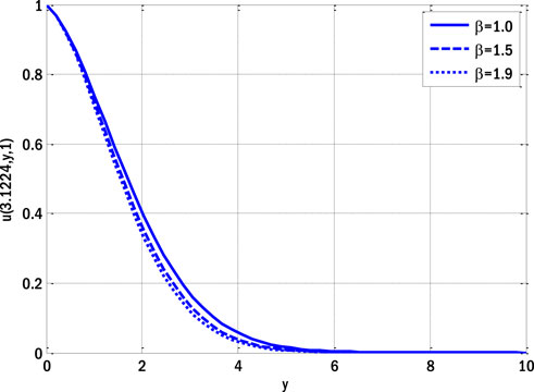
FIGURE 1. Effect of Casson parameter on velocity profile for the deterministic model using Re = 1, Gr_T = 0.4, Gr_C = 0.5, ε = 0.1, ε₁ = 0.1, Ha = 0.1, E₁ = 0.1, Pr = 0.9, Ec = 0.1, Sc = 0.9, γ = 0.1.

FIGURE 2

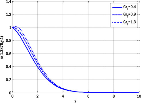
FIGURE 2. Effect of thermal Grashof number on velocity profile for the deterministic model using Re = 1, β = 1, Gr_C = 0.5, ε = 0.1, ε₁ = 0.1, Ha = 0.1, E₁ = 0.1, Pr = 0.9, Ec = 0.1, Sc = 0.9, γ = 0.1.

FIGURE 3

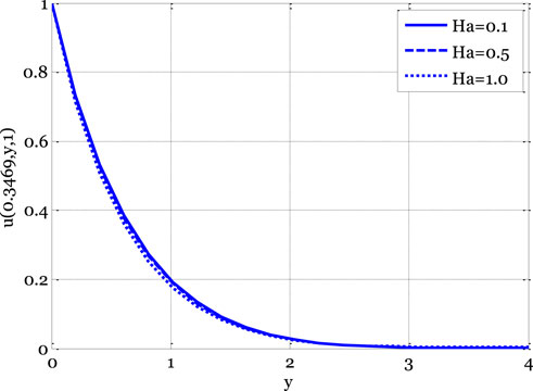
FIGURE 3. Effect of Hartmann number on velocity profile for the deterministic model using Re = 3, β = 1, Gr_C = 0.5, ε = 0.1, ε₁ = 0.1, Gr_T = 0.4, E₁ = 0.01, Pr = 0.9, Ec = 0.1, Sc = 0.9, γ = 0.1.

As the Hartmann number rises, the quality of a velocity profile deteriorates. Lorentz’s force increases in tandem with an increase in Hartmann’s number, slowing the flow and causing a decrease in the velocity profile. Figure 4 shows how the local electric parameter affects the velocity profile in the stochastic situation. Different parts of the domain display contrasting velocity profiles. Figure 5 depicts the temperature distribution as a function of the Eckert number. Stochastic analysis reveals a bimodal distribution of temperatures.

FIGURE 4

FIGURE 4. Effect of local electric parameter on velocity profile for the stochastic model using Re = 3, β = 1, Gr_C = 0.5, ε = 0.1, ε₁ = 0.1, Gr_T = 0.4, Ha = 1, Pr = 0.9, Ec = 0.1, Sc = 0.9, γ = 0.1, σ₁ = 0.9, σ₂ = 0.4, σ₃ = 0.3.

FIGURE 5

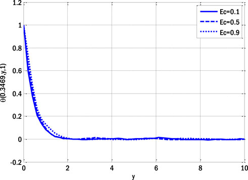
FIGURE 5. Effect of Eckert number on a temperature profile for the stochastic model using Re = 3, β = 1, Gr_C = 0.5, ε = 0.1, ε₁ = 0.1, Gr_T = 0.4, Ha = 0.1, Pr = 0.9, E₁ = 0.01, Sc = 0.9, γ = 0.1, σ₁ = 0.5, σ₂ = 0.4, σ₃ = 0.3, x₀ = 0.3469.

Nonetheless, as the boundary layer flows over the plates, the temperature profile typically increases as the Eckert number rises. The temperature profile variation as a function of minor parameters is illustrated in Figure 6. The temperature exhibits a dual effect by increasing minor parameters. The temperature profile increases for the deterministic model as small parameters increase, as the thermal conductivity also increases with small parameter values. Consequently, the temperature profile experiences an upward trend. The impact of the reaction rate parameter on the concentration profile of the stochastic model is illustrated in Figure 7. In the context of boundary layer flow over flat plates, the concentration profile typically decreases as the reaction rate parameters increase, according to the deterministic model. Figure 8 demonstrates the influence of a modest parameter introduced in variable mass diffusivity on the stochastic model’s concentration profile. Figure 9 shows the impact of the stochastic model’s velocity, temperature, and concentration profiles.

FIGURE 6

FIGURE 6. Effect of small parameter on a temperature profile for the stochastic model using Re = 3, β = 1, Gr_C = 0.5, Ec = 0.1, ε₁ = 0.1, Gr_T = 0.4, Ha = 0.1, Pr = 0.9, E₁ = 0.01, Sc = 0.9, γ = 0.1, σ₁ = 0.5, σ₂ = 0.4, σ₃ = 0.3, x₀ = 0.3469.

FIGURE 7

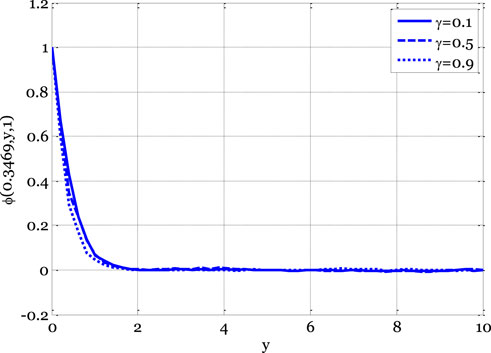
FIGURE 7. Effect of reaction rate parameter on concentration profile for the stochastic model using Re = 3, β = 1, Gr_C = 0.5, Ec = 0.1, ε₁ = 0.1, Gr_T = 0.4, Ha = 0.1, Pr = 0.9, E₁ = 0.01, Sc = 0.9, ε = 0.1, σ₁ = 0.5, σ₂ = 0.4, σ₃ = 0.3, x₀ = 0.3469.

FIGURE 8

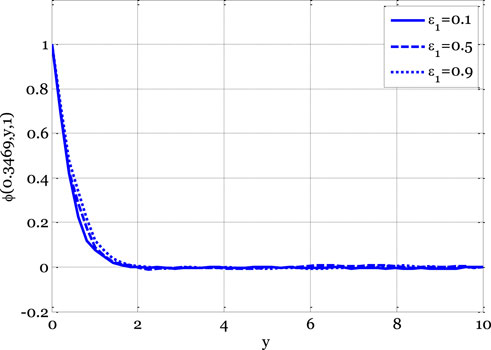
FIGURE 8. Effect of small parameter on concentration profile for the stochastic model using Re = 3, β = 1, Gr_C = 0.5, Ec = 0.1, γ = 0.1, Gr_T = 0.4, Ha = 0.1, Pr = 0.9, E₁ = 0.01, Sc = 0.9, ε = 0.1, σ₁ = 0.5, σ₂ = 0.4, σ₃ = 0.3, x₀ = 0.3469.

FIGURE 9

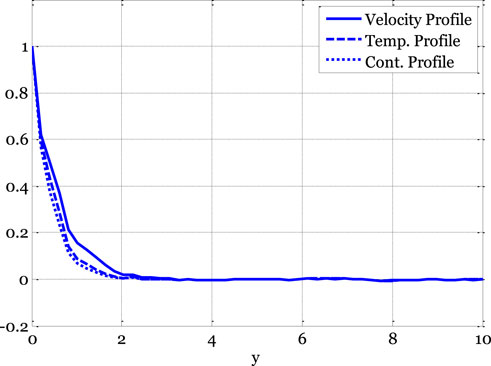
FIGURE 9. Velocity, temperature, and concentration profiles of the stochastic model using Re = 3, β = 1, Gr_C = 0.5, Ec = 0.9, γ = 0.1, Gr_T = 0.4, Ha = 0.1, Pr = 0.9, E₁ = 0.01, Sc = 0.9, ε₁ = 0.1, ε = 0.1, σ₁ = 0.5, σ₂ = 0.4, σ₃ = 0.3, x₀ = 0.3469, t_f = 1.

Figures 10, 11 show the mesh plots for the horizontal and vertical components of velocity profiles for the oscillatory boundary beneath contours. Because the time coordinate determines the oscillation border, oscillatory behaviour can be observed along the time coordinate. The stochastic effect on the horizontal velocity component is not noticeable or minor. Nonetheless, the variation of Wiener process term(s) is visible in the contours for the horizontal velocity component. The mesh plot for the temperature profile over spatial and temporal coordinates is shown in Figure 12. Figure 12 depicts the influence of the oscillatory boundary on the velocity profile and the effect of the Wiener process term. In Figures 13, 14, the mesh plots beneath contours for the horizontal component of velocity and concentration profiles are displayed over the spatial coordinates. Figure 15 compares the proposed stochastic and existing Euler Maruyama schemes for the problem considered in this contribution. Figure 16 shows the norm of difference between numerical and exact solutions for the first example studies in [48]. Different mesh sizes are considered for the study. The mesh sizes are $25\times 25,35\times 35,45\times 45,55\times 55$ along $x$ and $y$ directions. This Figure 16 also shows that error decreases by increasing mesh size. The error is calculated by finding the $L_2$ norm for the difference between numerical and exact solutions at the final time.

FIGURE 10

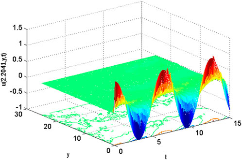
FIGURE 10. Mesh plot underneath contours for the horizontal component of velocity profile on spatial and temporal coordinates of the stochastic model using Re = 3, β = 1, Gr_C = 0.5, Ec = 0.1, γ = 0.1, Gr_T = 0.4, Ha = 0.1, Pr = 0.9, E₁ = 0.01, Sc = 0.9, ε₁ = 0.1, ε = 0.1, σ₁ = 0.5, σ₂ = 0.4, σ₃ = 0.3, L_x = 27, u_w = cos(t).

FIGURE 11

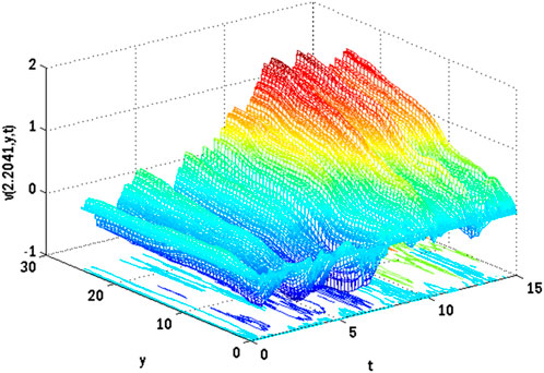
FIGURE 11. Mesh plot underneath contours for the vertical component of velocity profile on spatial and temporal coordinates of the stochastic model using Re = 3, β = 1, Gr_C = 0.5, Ec = 0.1, γ = 0.1, Gr_T = 0.4, Ha = 0.1, Pr = 0.9, E₁ = 0.01, Sc = 0.9, ε₁ = 0.1, ε = 0.1, σ₁ = 0.5, σ₂ = 0.4, σ₃ = 0.3, L_x = 27, u_w = cos(t).

FIGURE 12

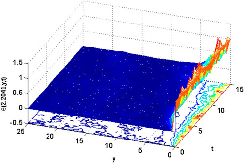
FIGURE 12. Mesh plot underneath contours plot for temperature on spatial and temporal coordinates of the stochastic model using Re = 3, β = 1, Gr_C = 0.5, Ec = 0.1, γ = 0.1, Gr_T = 0.4, Ha = 0.1, Pr = 0.9, E₁ = 0.01, Sc = 0.9, ε₁ = 0.1, ε = 0.1, σ₁ = 0.5, σ₂ = 0.4, σ₃ = 0.3, L_x = 27, u_w = cos(t).

FIGURE 13

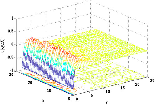
FIGURE 13. Mesh plot underneath contours for the horizontal component of velocity profile on spatial coordinates of the stochastic model using Re = 3, β = 1, Gr_C = 0.5, Ec = 0.1, γ = 0.1, Gr_T = 0.4, Ha = 0.1, Pr = 0.9, E₁ = 0.01, Sc = 0.9, ε₁ = 0.1, ε = 0.1, σ₁ = 0.5, σ₂ = 0.4, σ₃ = 0.3, L_x = 27, u_w = cos(t).

FIGURE 14

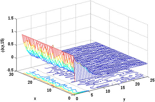
FIGURE 14. Mesh plot underneath contours for concentration profile on spatial coordinates of the stochastic model using Re = 3, β = 1, Gr_C = 0.5, Ec = 0.1, γ = 0.1, Gr_T = 0.4, Ha = 0.1, Pr = 0.9, E₁ = 0.01, Sc = 0.9, ε₁ = 0.1, ε = 0.1, σ₁ = 0.5, σ₂ = 0.4, σ₃ = 0.3, L_x = 27, u_w = cos(t).

FIGURE 15

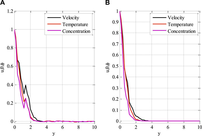
FIGURE 15. Comparison of (A) proposed scheme and stochastic scheme (B) Euler Maruyama method using Re = 3, β = 1, Gr_T = 0.4, Gr_C = 0.5, ε = 0.1, ε₁ = 0.1, H₀ = 0.1, E₁ = 0.01, Pr = 0.9, Ec = 0.9, Sc = 0.9, γ = 0.1, σ₁ = 0.9, σ₂ = 0.7, σ₃ = 1.3.

FIGURE 16

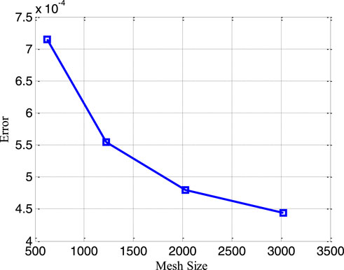
FIGURE 16. Error over mesh size using. t_f (final time) = 0.07, Nt (No. of time levels) = 1000.

6 Conclusion

The precise representation and simulation of unsteady non-Newtonian mixed convective flows incorporating varying thermal conductivity and mass diffusivity provide a noteworthy obstacle within fluid dynamics. The present study has introduced an innovative strategy to tackle this obstacle by devising and executing a novel stochastic finite difference scheme. The main objective of this study was to develop a robust computational tool that can effectively model the stochastic characteristics of intricate fluid flow phenomena. This tool aims to improve our comprehension, prediction, and optimization of systems in which these phenomena are present. By investigating the mathematical underpinnings and computational execution of our innovative approach alongside a sequence of numerical trials, we have acquired significant knowledge regarding the possibilities and constraints of the scheme. Including stochastic aspects in the modelling process significantly enhances the precision and dependability of simulations, particularly in scenarios involving systems inherently characterized by unpredictability and uncertainties. A stochastic numerical approach has been created to solve stochastic time-dependent partial differential equations. Stages of prediction and correction form the basis of the plan.

In contrast, the corrector stage approximates the integral of the Wiener process term and gives second-order precision for the non-stochastic portion. The paper also discussed the issue of non-Newtonian fluid flow over flat and oscillatory plates subject to the influence of temperature and mass diffusivity variations. In summary, the arguments might be stated as.

1. The velocity profile declined as the values of the Casson parameter and Hartmann number increased.

2. The velocity has dual behaviour by rising local electric parameters.

3. The temperature and concentration profiles have dual behaviours by rising small parameters that appeared in variable thermal conductivity and mass diffusivity.

The results of our study have indicated that the newly developed stochastic finite difference scheme holds significant value as a supplementary tool for academics and engineers engaged in fluid dynamics. The proposed methodology demonstrates a high level of efficacy in managing the challenges posed by unsteady non-Newtonian mixed convective flows with varying thermal conductivity and mass diffusivity but also contributes to a more comprehensive comprehension of the influence of stochastic elements within these intricate systems. Consequently, this scheme can enhance decision-making processes in designing and optimizing numerous processes across several disciplines, such as chemical engineering, environmental science, and fluid mechanics. We expect this unique technique to be widely adopted as we develop and expand. We believe it can advance our understanding and application of complex, stochastic fluid flow processes.

Data availability statement

The original contributions presented in the study are included in the article/Supplementary Material, further inquiries can be directed to the corresponding author.

Author contributions

MA: Conceptualization, Funding acquisition, Investigation, Project administration, Software, Supervision, Writing–original draft, Writing–review and editing. KA: Conceptualization, Formal Analysis, Methodology, Resources, Validation, Visualization, Writing–original draft, Writing–review and editing. YN: Conceptualization, Data curation, Formal Analysis, Investigation, Software, Writing–original draft, Writing–review and editing.

Funding

The author(s) declare that no financial support was received for the research, authorship, and/or publication of this article. This research did not receive any specific grant from public, commercial, or not-for-profit funding agencies.

Acknowledgments

The authors wish to express their gratitude to Prince Sultan University for facilitating the publication of this article through the Theoretical and Applied Sciences Lab.

Conflict of interest

The authors declare that the research was conducted in the absence of any commercial or financial relationships that could be construed as a potential conflict of interest.

Publisher’s note

All claims expressed in this article are solely those of the authors and do not necessarily represent those of their affiliated organizations, or those of the publisher, the editors and the reviewers. Any product that may be evaluated in this article, or claim that may be made by its manufacturer, is not guaranteed or endorsed by the publisher.

References

1. Brinkman HC. Heat effects in capillary flow I. Appl Sci (1951) 2:120–4. doi:10.1007/bf00411976

CrossRef Full Text | Google Scholar

2. Jambal O, Shigechi T, Davaa G, Momoki S. Effects of viscous dissipation and fluid axial heat conduction on heat transfer for non-Newtonian fluids in duct with uniform wall temperature. Int Commun Heat Mass Transfer (2005) 32:1165–73. doi:10.1016/j.icheatmasstransfer.2005.07.002

CrossRef Full Text | Google Scholar

3. Das SK, Choy SU, Yu W, Praveen T. Nanofluids: science and technology. Hoboken, New Jersey, United States: John Wiley and Sons (2007).

Google Scholar

4. Marquis FDS, Chianti LPF. Improving the heat transfer of nanofluids and nanolubricants with carbon nanotubes. J Manag (2005) 57:32–43. doi:10.1007/s11837-005-0180-4

CrossRef Full Text | Google Scholar

5. Choi SUS. Enhancing thermal conductivity of fluids with nanoparticles. Dev Appl Non-newtonian Flows (1995) 231:99–105.

Google Scholar

6. Aziz MAE. Unsteady mixed convection heat transfer along a vertical stretching surface with variable viscosity and viscous dissipation. J Egypt Math. Soc. (2014) 22:529–37. doi:10.1016/j.joems.2013.11.005

CrossRef Full Text | Google Scholar

7. Ho CJ, Chen MW, Li ZW. Numerical simulation of natural convection of nanofluid in a square enclosure: effects due to uncertainties of viscosity and thermal conductivity. Int J Heat Mass Transf (2008) 51:4506–16. doi:10.1016/j.ijheatmasstransfer.2007.12.019

CrossRef Full Text | Google Scholar

8. Yang YT, Lai FH. Numerical study of heat transfer enhancement with the use of nanofluids in radial flow cooling system. Int J Heat Mass Transf (2010) 53:5895–904. doi:10.1016/j.ijheatmasstransfer.2010.07.045

CrossRef Full Text | Google Scholar

9. Nasrin R, Alim MA. Finite element simulation of forced convection in a flat plate solar collector: influence of nanofluid with double nanoparticles. J Appl Fluid Mech (2014) 7(3):543–57. doi:10.36884/JAFM.7.03.21416

CrossRef Full Text | Google Scholar

10. Nie XB, Chen SY, Robbins M. A continuum and molecular dynamics hybrid method for micro-and nanofluid flow. J Fluid Mech (2004) 500:55–64. doi:10.1017/s0022112003007225

CrossRef Full Text | Google Scholar

11. Chougule SS, Sahu SK. Model of heat conduction in hybrid nanofluid. In: 2013 IEEE International Conference on Emerging Trends in Computing, Communication and Nanotechnology (ICECCN); March, 2013; Tirunelveli, India (2013). p. 337–41.

CrossRef Full Text | Google Scholar

12. Labib MN, Nine MJ, Afrianto H, Chung H, Jeong H. Numerical investigation on effect of base fluids and hybrid nanofluid in forced convective heat transfer. Int J Therm Sci (2013) 71:163–71. doi:10.1016/j.ijthermalsci.2013.04.003

CrossRef Full Text | Google Scholar

13. Elbarbary EME, Elagzery NS. Chebyshev finite difference method for the effects of variable viscosity and variable thermal conductivity on heat transfer on moving surfaces with radiation. Int J Therm Sci (2004) 43:889–99. doi:10.1016/j.ijthermalsci.2004.01.008

CrossRef Full Text | Google Scholar

14. Saleem AM. Variable viscosity and thermal conductivity effects on. MHD Flow Heat Transfer Viscoelastic Fluid Over A Stretching Sheet (2007) 4:315–22. doi:10.1016/j.physleta.2007.04.104

CrossRef Full Text | Google Scholar

15. Hashim A, Hamid , Khan M. Unsteady mixed convection flow of Williamson nanofluid with heat transfer in the presence of variable thermal conductivity and magnetic field. J Mol Liquids (2018) 260:436–46. doi:10.1016/j.molliq.2018.03.079

CrossRef Full Text | Google Scholar

16. Malik MY, Hussain A, Nadeem S. Boundary layer flow of an Eyring-powel model fluid due to a stretching cylinder with variable viscosity. Sci Iran (2013) 20:313–21. doi:10.1016/j.scient.2013.02.028

CrossRef Full Text | Google Scholar

17. Umavathi JC, Sheremet MA, Mohiuddin S. Combined effect of variable viscosity and thermal conductivity on mixed convection flow of a viscous fluid in a vertical channel in the presence of first order chemical reaction. Eur J Mech B Fluids (2016) 58:98–108. doi:10.1016/j.euromechflu.2016.04.003

CrossRef Full Text | Google Scholar

18. Akinbobola TE, Okoya SS. The flow of second grade fluid over a stretching sheet with variable thermal conductivity and viscosity in the presence of heat source/sink. J Niger Math Soc (2015) 34:331–42. doi:10.1016/j.jnnms.2015.10.002

CrossRef Full Text | Google Scholar

19. Muthucumaraswamy R. Effects of chemical reaction on moving isothermal vertical plate with variable mass diffusion. Theore Aplie Mech (2003) 3:209–20. doi:10.2298/tam0303209m

CrossRef Full Text | Google Scholar

20. Muthucumaraswamy R, Janakiraman B. MHD and radiation effects on moving isothermal vertical plate with variable mass diffusion. Theoret Appl Mech (2006) 1:17–29. doi:10.2298/tam0601017m

CrossRef Full Text | Google Scholar

21. Jia X, Zeng F, Gu Y. Semi analytical solution to one-dimensional advection-diffusion equations with variable diffusion coefficient and variable flow velocity. Appl Math Comput (2013) 221:268–81. doi:10.1016/j.amc.2013.06.052

CrossRef Full Text | Google Scholar

22. Li C, Guo H, Tian X. Time-domain finite element analysis to nonlinear transient responses of generalized diffusion-thermo elasticity with variable thermal conductivity and diffusivity. Int J Mech Sci (2017) 131:234–44. doi:10.1016/j.ijmecsci.2017.07.008

CrossRef Full Text | Google Scholar

23. Qureshi IH, Nawaz M, Rana S, Zubair T. Galerkin finite element study on the effects of variable thermal conductivity and variable mass diffusion conductance on heat and mass transfer. Commun Theor Phys (2018) 70:049–59. doi:10.1088/0253-6102/70/1/49

CrossRef Full Text | Google Scholar

24. Khan M, Salahuddin T, Tanveer A, Malik MY, Hussain A. Change in internal energy of thermal diffusion stagnation point Maxwell nanofluid flow along with solar radiation and thermal conductivity. Chin J Chem Eng (2018) 27:2352–8. doi:10.1016/j.cjche.2018.12.023

CrossRef Full Text | Google Scholar

25. Kumri M, Nath G. Mixed convection boundary layer flow over a thin vertical cylinder with localized injection/suction and cooling/heating. Int J Heat Mass Transfer (2004) 47:969–76. doi:10.1016/j.ijheatmasstransfer.2003.08.014

CrossRef Full Text | Google Scholar

26. Ishak A, NazarPop RI. Boundary layer flow over a continuously moving thin needle in a parallel free stream. Chienese Phys Lett (2007) 24:2895–7. doi:10.1088/0256-307X/24/10/051

CrossRef Full Text | Google Scholar

27. Chen JLS, Smith TN. Forced convection heat transfer from non-isothermal thin needles. J Heat Transfer (1978) 100:358–62. doi:10.1115/1.3450809

CrossRef Full Text | Google Scholar

28. Ahmad R, Mustafa M, Hina S. Bungirono model for fluid flow around a moving thin needle in a flowing nano fluid, a numerical study. Chin J Phys (2017) 55:1264–74. doi:10.1016/j.cjph.2017.07.004

CrossRef Full Text | Google Scholar

29. Mittal AS, Patel HR. Influence of thermophoresis and brownian motion on mixed convection two dimensional MHD Casson fluid flow with nonlinear radiation and heat generation. Physica A (2020) 537:122710. doi:10.1016/j.physa.2019.122710

CrossRef Full Text | Google Scholar

30. Animasaun IL. Double diffusive unsteady convective micropolar flow past a vertical porous plate moving through binary mixture using modified Boussinesq approximation. Ain Shams Eng J (2016) 7:755–65. doi:10.1016/j.asej.2015.06.010

CrossRef Full Text | Google Scholar

31. Animasaun IL. Dynamics of unsteady MHD convective flow with thermophoresis of particles and variable thermo-physical properties past a vertical surface moving through binary mixture. Open J Fluid Dyn (2015) 5:106–20. doi:10.4236/ojfd.2015.52013

CrossRef Full Text | Google Scholar

32. Shah NA, Animasaun IL, Ibraheem RO, Babatunde HA, Sandeep N, Pop I. Scrutinization of the effects of grashof number on the flow of different fluids driven by convection over various surfaces. J Mol Liquids (2018) 249:980–90. doi:10.1016/j.molliq.2017.11.042

CrossRef Full Text | Google Scholar

33. Animasaun IL, Koriko OK, Mahanthesh B, Dogonchi AS. A note on the signif-icance of quartic autocatalysis chemical reaction on the motion of air conveying dust particles. Z Nat.forsch (2019) 10:879–904. doi:10.1515/zna-2019-0180

CrossRef Full Text | Google Scholar

34. Animasaun IL, Ibraheem RO, Mahanthesh B, Babatunde HA. A meta-analysis the effects of haphazard motion of tiny/nano sized particles on the dynamics and other physical properties of some fluids. Chin J. Phys. (2019) 60:676–687. doi:10.1016/j.cjph.2019.06.007

CrossRef Full Text | Google Scholar

35. Koriko OK, Adegbie KS, Animasaun IL, Ijirimoye AF. Comparative analysis between three–dimensional flow of water conveying alumina nanoparticles and water conveying alumina–iron(III) oxide nanoparticles in the presence of lorentz force. Arab J Sci Eng (2020) 45:455–64. doi:10.1007/s13369-019-04223-9

CrossRef Full Text | Google Scholar

36. Tanuja TN, Kavitha L, Ur Rehman K, Shatanawi W, Varma SVK, Kumar GV. Heat transfer in magnetohydrodynamic Jeffery–Hamel molybdenum disulfide/water hybrid nanofluid flow with thermal radiation: a neural networking analysis. Numer Heat Transfer, A: Appl (2024) 1–19. doi:10.1080/10407782.2023.2300744

CrossRef Full Text | Google Scholar

37. Abbas N, Ali M, Shatanawi W, Hasan F. Unsteady micropolar nanofluid flow past a variable riga stretchable surface with variable thermal conductivity. Heliyon (2024) 10(1):e23590. doi:10.1016/j.heliyon.2023.e23590

PubMed Abstract | CrossRef Full Text | Google Scholar

38. Rehman A, Khun MC, Khan D, Shah K, Abdeljawad T. Stability analysis of the shape factor effect of radiative on MHD couple stress hybrid nanofluid. South Afr J Chem Eng (2023) 46:394–403. doi:10.1016/j.sajce.2023.09.004

CrossRef Full Text | Google Scholar

39. Tessitore G. Existence, uniqueness and space regularity of the adapted solutions of a backward SPDE. Stoch Anal Appl (1996) 14:461–86. [Google Scholar] [CrossRef]. doi:10.1080/07362999608809451

CrossRef Full Text | Google Scholar

40. Dozzi M, López-Mimbela JA. Finite-time blowup and existence of global positive solutions of a semilinear SPDE. Stoch Process Appl (2010) 120:767–76. [Google Scholar] [CrossRef] [Green Version]. doi:10.1016/j.spa.2009.12.003

CrossRef Full Text | Google Scholar

41. Xiong J, Yang X. Existence and pathwise uniqueness to an SPDE driven by a-stable colored noise. Stoch Process Appl (2019) 129:2681–722. [Google Scholar] [CrossRef]. doi:10.1016/j.spa.2018.08.003

CrossRef Full Text | Google Scholar

42. Altmeyer R, Bretschneider T, Janák J, Reiß M. Parameter estimation in an SPDE model for cell repolarization SIAM/ASA. J Uncertain Quantif (2022) 10:179–99. [Google Scholar] [CrossRef]. doi:10.1137/20M1373347

CrossRef Full Text | Google Scholar

43. Gyöngy I, Martínez T. On numerical solution of stochastic partial differential equations of elliptic type Sto-chastics: an International. J Probab Stoch Process (2006) 78:213–31. [Google Scholar] [CrossRef]. doi:10.1080/17442500600805047

CrossRef Full Text | Google Scholar

44. Kamrani M, Hosseini SM. The role of coefficients of a general SPDE on the stability and convergence of a finite difference method. J Comput Appl Math (2010) 234:1426–34. doi:10.1016/j.cam.2010.02.018

CrossRef Full Text | Google Scholar

45. Yasin MW, Iqbal MS, Ahmed N, Akgül A, Raza A, Rafiq M, et al. Numerical scheme and stability analysis of stochastic Fitzhugh-Nagumo model. Results Phys (2022) 32:105023. doi:10.1016/j.rinp.2021.105023

CrossRef Full Text | Google Scholar

46. Yasin MW, Iqbal MS, Seadawy AR, Baber MZ, Younis M, Rizvi ST. Numerical scheme and analytical solutions to the stochastic nonlinear advection diffusion dynamical model. Int J Nonlinear Sci Numer Simul (2021) 24:467–87. doi:10.1515/ijnsns-2021-0113

CrossRef Full Text | Google Scholar

47. Allen EJ, Novosel SJ, Zhang Z. Finite element and difference approximation of some linear stochastic partial differential equations. Stoch Int J Probab Stoch Process (1998) 64:117–42. doi:10.1080/17442509808834159

CrossRef Full Text | Google Scholar

48. Fu-le Li , Wu Z-ku, Ye C-rong. A finite difference solution to a two-dimensional parabolic inverse problem. Appl Math Model (2012) 36(5):2303–13. doi:10.1016/j.apm.2011.08.025

CrossRef Full Text | Google Scholar