 Zhongbin Luo
 Yanqiu Bi3,4*
 Xun Yang
 Yong Li
- 1China Merchants Chongqing Communications Research and Design Institute Co., Ltd., Chongqing, China
- 2Research and Development Center of Transport Industry of Self-Driving Technology, Chongqing, China
- 3National and Local Joint Engineering Research Center of Transportation Civil Engineering Materials, Chongqing Jiaotong University, Chongqing, China
- 4School of Civil Engineering, Chongqing Jiaotong University, Chongqing, Shandong, China
- 5College of Computer Science, Chongqing University, Chongqing, China
- 6Key Laboratory of Dependable Service Computing in Cyber Physical Society, Ministry of Education, Chongqing University, Chongqing, China
Addressing the need for vehicle speed measurement in traffic surveillance, this study introduces an enhanced scheme combining YOLOv5s detection with Deep SORT tracking. Tailored to the characteristics of highway traffic and vehicle features, the dataset data augmentation process was initially optimized. To improve the detector’s recognition capabilities, the Swin Transformer Block module was incorporated, enhancing the model’s ability to capture local regions of interest.
1 Introduction
Intelligent Transportation Systems (ITS) have been widely applied to practical traffic scenarios such as highways, urban roads, tunnels, and bridges. This integration owes much to the convergence of various technologies, including pattern recognition, video image processing, and network communication [1, 2]. Vehicle speed is a crucial parameter that directly reflects the state of traffic [3, 4]. Meanwhile, in highly complex traffic monitoring scenarios and under special weather conditions, intelligent transportation monitoring systems face numerous significant challenges. In addressing the issue of vehicle speeding, the measurement of vehicle speed can provide vital data for traffic management authorities. Accurate measurement of vehicle target speed is one of the challenges faced by traffic monitoring systems.
Traditional vehicle speed detection primarily utilizes inductive loop detection, laser detection, and radar detection. These methods are well-developed and commonly used in traffic systems. However, traditional detection methods have the following disadvantages: (1) the required equipment is expensive; (2) the equipment is installed under the road surface, leading to high subsequent maintenance costs and maintenance not only affects traffic but also damages road structure. Video-based vehicle speed detection leverages numerous traffic video monitoring devices, significantly overcoming the high costs and difficult maintenance issues associated with traditional speed detection methods. The vehicle speed detection system can be categorized into two types: one type focuses on accurate speed monitoring systems (such as speed camera applications) [5, 6], and the other type, though less precise, can be used to estimate traffic speed (such as traffic camera application scenarios) [7, 8]. This classification system takes into account the intrinsic parameters of the camera (such as sensor size and resolution, focal length), as well as extrinsic parameters (such as the camera’s position relative to the road surface, drone-based cameras, etc.), and the number of cameras (monocular, stereo, or multiple cameras).
Through these parameters, the actual scene on the image plane can represent one or multiple lanes, as well as the relative position of vehicles to the camera, ultimately yielding one of the most critical variables: the ratio of pixels to road segment length, i.e., the road length each pixel represents. Due to the perspective projection model, this ratio is directly proportional to the square of the camera’s distance, implying that measurements over long distances have poor accuracy. Accurate estimation of the camera’s intrinsic and extrinsic parameters is required to provide measurements in the actual coordinate system. The most common approach is soft calibration, which involves calibrating intrinsic parameters in a verification laboratory or using sensor and lens characteristics, and estimating the rigid transformation between the camera and the road surface using manual [9, 10] or automatic [11] methods.
Hard calibration involves estimating both the intrinsic and extrinsic parameters of the camera, which can be done either manually [12] or automatically [13–15]. In certain limited scenarios, some details of camera calibration may be overlooked, such as the exact position of the camera, anchoring systems, gantries. Since cameras are mostly static (except for drone cameras), vehicle detection is most often addressed by modeling the background [16–18]. Other methods are feature-based, such as detecting vehicle license plates [19, 20] or other characteristics [21–23].
Recently, learning-based approaches have become increasingly popular for recognizing vehicles in images [24, 25]. The ability to track vehicles with smooth and stable trajectories is a key issue in handling vehicle speed detection. Vehicle tracking can be divided into three different categories: The first category is feature-based [26–28], where tracking originates from a set of features of the vehicle (such as optical flow). The second category focuses on tracking the centroid of a vehicle’s blob or bounding box [29, 30]. The third category concentrates on tracking the entire vehicle [31, 32] or its specific parts (such as the license plate [33, 34]).
The prerequisite for speed measurement is the effective assessment of distance. In monocular vision systems, the estimation of vehicle distance typically relies on specific constraints and methods. These include: (1) Flat road assumption and homography-based methods, which assume that the road is flat and apply a mathematical transformation known as homography [35, 36], helping in mapping the view of a scene from one perspective to another, which is crucial for estimating distances in 2D images; (2) Detection of lines and specific areas [37, 38]. By detecting lines and specific areas, designed detection lines and areas can be overlaid on the real-world view, providing a reference scale for measuring distances; (3) Use of prior knowledge about object dimensions, utilizing the known dimensions of certain objects to estimate distances. For instance, knowing the standard sizes of license plates ([39, 40]) or the average dimensions of vehicles [41] can assist in calibrating distance measurements. However, these monocular methods have limitations, which are addressed in stereo vision systems. In stereo vision systems [42], two cameras are used to capture the same scene from slightly different angles, similar to human binocular vision. This setup allows for more accurate depth perception and distance estimation, as it mimics the way.
Currently, speed detection is primarily divided into macroscopic traffic flow speed and individual vehicle speed. Macroscopic traffic flow speed detection is based on a specific road section, using the length of the section and travel time to estimate the average speed of the segment [43, 44]. Individual vehicle speed detection focuses on the micro-level speed of the vehicle itself, presenting greater technical challenges. This process requires prior knowledge of the camera’s frame rate or accurate timestamps for each image to calculate the time between measurements. Utilizing consecutive or non-consecutive [45] images to estimate speed is a key factor impacting accuracy. In summary, whether in traffic flow speed or individual vehicle speed detection, factors such as the method of image capture (continuous or non-continuous), frame rate, timestamp accuracy, and the integration of various measurement data need to be carefully considered. The selection method and precision of these factors directly affect the accuracy of speed estimation.
In summary, vision-based vehicle speed detection involves the entire process of camera calibration, distance estimation, and speed estimation. However, the calibration process for monocular vision cameras is complex, the accuracy of distance estimation is relatively poor, and the precision of individual vehicle speed estimation needs improvement. Currently, there are few instances of rapidly detecting and stably tracking vehicle instantaneous speeds solely through video recognition technology, which limits the broader application of video recognition technologies in the field of traffic safety. Therefore, this study introduces an enhanced scheme that combines YOLOv5s detection with Deep SORT tracking, targeting the need for vehicle speed measurement in traffic monitoring. The dataset data expansion process is preliminarily optimized based on the characteristics of highway traffic and vehicle features. The Swin Transformer Block module is introduced to improve the detector’s recognition capabilities and enhance the model’s ability to capture areas of interest. The
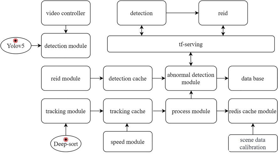
FIGURE 1. Algorithm framework diagram.
2 Improved YOLOv5s + DeepSORT algorithm for highway vehicle detection and tracking
2.1 Construction of vehicle target dataset
2.1.1 Characteristics of highway traffic scenarios
There are typically four categories of common highway traffic scenarios, as shown in Figure 2.
(a) Scene variations, as the setup of traffic monitoring varies, so do the monitoring angles and heights. For instance, the monitoring angle and scene characteristics inside a tunnel differ greatly from those on a highway, leading to significantly reduced detection accuracy and numerous false detections of vehicle targets, as shown in Figure 2A.
(b) The same scene at different times also exhibits significant differences. With changes in time, the brightness and visibility of scene images vary. The characteristics of vehicle targets at night are particularly difficult to capture due to the substantial interference from vehicle lights at night, making it hard to accurately obtain the body contours of target vehicles. If the dataset does not include such special night scene data, the detection results are not ideal Figure 2B.
(c) Vehicle targets at different positions in the image will have obvious deformation. The same vehicle target will undergo significant size deformation from distant to closer positions in the image, affecting the detection accuracy of small targets. The red boxes in Figure 2C indicate significant deformations of the same vehicle target at different locations.
(d) On actual roads, there is a widespread occurrence of vehicle occlusion, which can lead to multiple targets being detected as one, resulting in missed and false detections. The red boxes in Figure 2D represent situations where vehicles are obstructing each other.
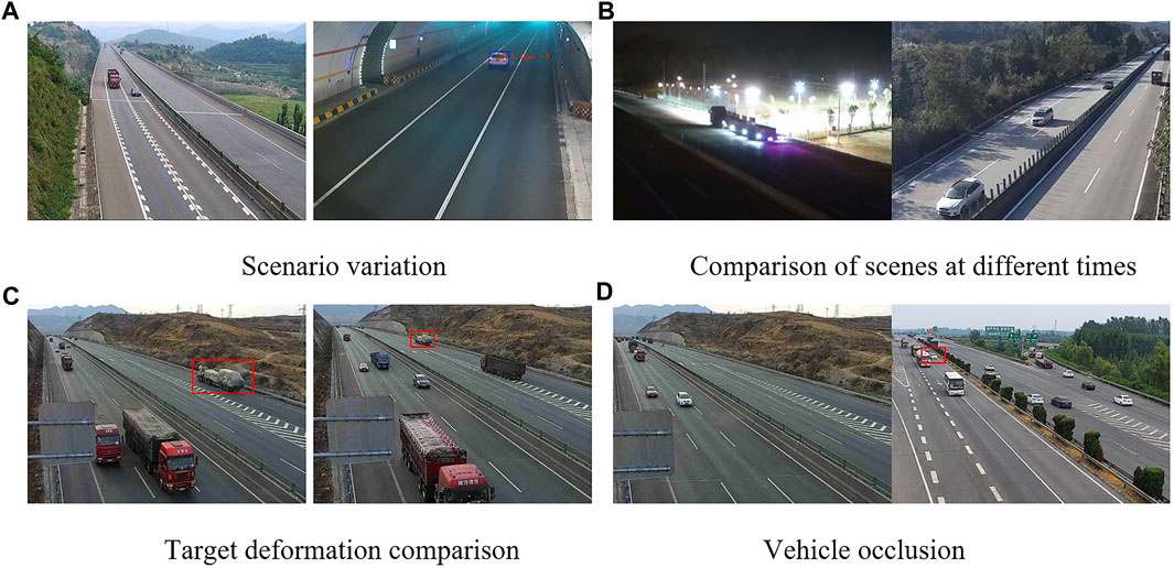
FIGURE 2. Common issues in target vehicle detection.
The existence of these four types of issues makes large public datasets such as COCO and VOC unsuitable for the perspectives captured by highway cameras, leading to a large number of false positives and missed detections of target vehicles.
2.1.2 Data preparation
Given the relatively uniform types of motor vehicles in highway scenarios, vehicles are generally classified into three categories: Car, Bus, and Truck. Car mainly refer to passenger vehicles with seating for fewer than seven people; Bus mainly include commercial buses, public transport buses, etc.; Truck primarily refer to small, medium, and large trucks, trailers, and various types of special-purpose vehicles as shown in Table 1. By collecting datasets from different scenes on highways and manually labeling them using the labelImg tool, a dataset in YOLO format was ultimately created.
The specific process includes: (1) Data Collection: Collect representative image data covering various scenes and angles of target categories. (2) Data Division: Divide the dataset into training, validation, and test sets, typically in a certain ratio, to ensure the independence and generalizability of the data. (3) Bounding Box Annotation: Annotate each target object with a bounding box, usually represented by a rectangle, including the coordinates of the top-left and bottom-right corners. Category Labeling: Assign corresponding category labels to each target object, identifying the category to which the object belongs. During dataset annotation, rectangular bounding boxes encompassing the entire vehicle are marked, with each side fitting closely to the vehicle. Annotation is not performed when the occlusion exceeds 50%, the vehicle type is indistinguishable, or the size is below 10*10 pixels. Furthermore, in cases where vehicles are truncated, the truncation is not considered to affect the overall annotation. Trucks used for transportation are uniformly annotated, without separately marking the vehicles on them.
2.1.3 Data augmentation
To enhance the accuracy and generalization capability of model training, data augmentation techniques are employed, tailored to the characteristics of highway traffic environments and vehicle features. These techniques include Mosaic, Random_perspective, Mixup, HSV, Flipud, Fliplr, as shown in Figure 3.
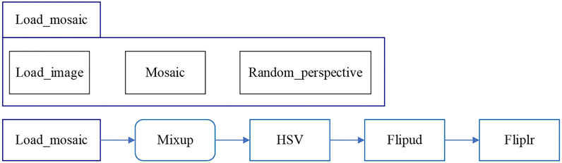
FIGURE 3. Data augmentation Flowchart.
2.2 Optimization of object detection network
In response to the identified issues with YOLOv5 in highway vehicle detection, the following optimizations were made to enhance the accuracy of vehicle detection: (1) Incorporating the Swin Transformer Block module to improve the model’s ability to capture information from local areas of interest; (2) Utilizing
2.2.1 Introduction of swin transformer block
To address the shortcomings of traditional YOLOv5 in traffic object detection, the Swin Transformer Block module is introduced for optimization.
The Swin Transformer network [46], proposed in 2021, is a Transformer network enhanced with a local self-attention mechanism. It has stronger dynamic computation capabilities compared to convolutional neural networks, with enhanced modeling capacity, and can adaptively compute both local and global pixel relationships, making it highly valuable for widespread use.
The core modules of the Transformer Block overall architecture are the Window-based Multi-Head Self-Attention layer (W-MSA) and the Shifted Window-based Multi-Head Self-Attention layer (SW-MSA). By restricting attention computation within a window, the network not only introduces the locality of convolution operations but also saves computational resources, resulting in good performance.
This article proposes the integration of the Swin Transformer Block structure into the backbone feature extraction network and neck feature fusion, utilizing the efficient self-attention mechanism module to fully explore the potential of feature representation. The improved YOLOv5 network incorporating the Swin Transformer Block module is shown in Figure 4, named SwinTransYOLOv5 network.
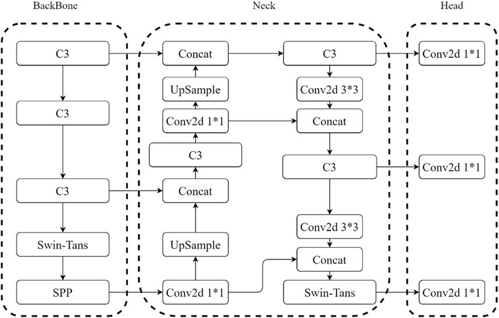
FIGURE 4. SwinTransYOLOv5 network structure diagram.
2.2.2 Improvement of loss function
YOLOv5s employs
In the formula,
In the formula,
In the formula,
Compared to the
2.2.3 Activation function
Changing the activation function can significantly enhance recognition performance. Activation functions are categorized into saturated and non-saturated types. The primary advantages of using non-saturated activation functions are twofold [47]: firstly, they effectively address the vanishing gradient problem, which becomes more severe with saturated activation functions; secondly, they can accelerate the convergence speed. After comparing the pros, cons, and characteristics of various activation functions without significantly increasing computational load, as shown in Table 2, the Leaky ReLU activation function in YOLOv5 was replaced with the Mish activation function.
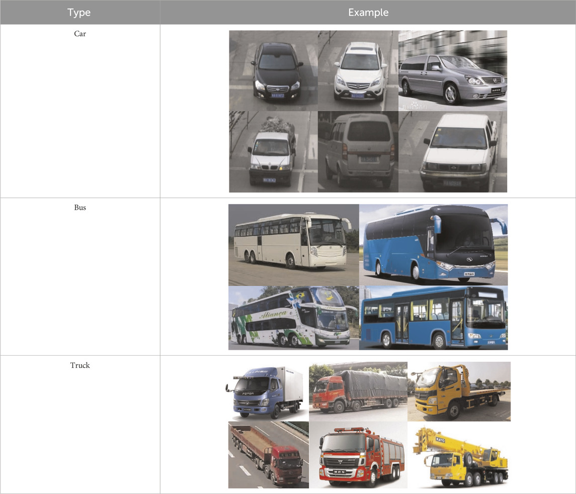
TABLE 1. Dataset categorization.
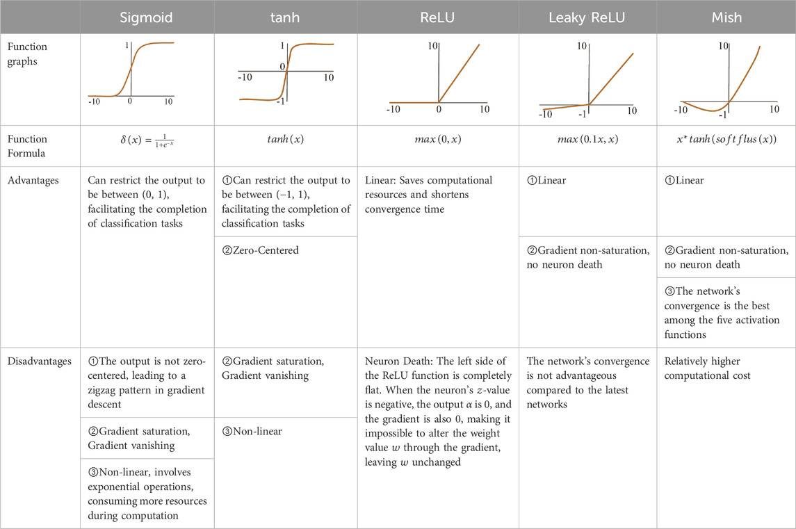
TABLE 2. Comparison of common activation functions.
2.3 Optimization of deep SORT for vehicle tracking
The multi-object online tracking algorithm SORT [48] (Simple Online and Realtime Tracking) utilizes Kalman filtering and Hungarian matching, using the
2.3.1 Tracking processing and state estimation
Deep SORT uses an 8-dimensional state space
(1) Mahalanobis Distance
The Mahalanobis distance is used to evaluate the predicted Kalman state and the new state, as shown in Eq. 4.
Considering the continuity of motion, detections are filtered using this Mahalanobis distance, with the 0.95 quantile of the chi-square distribution as the threshold value, defining a threshold function, as shown in Eq. 5.
(2) Appearance features
While Mahalanobis distance is a good measure of association when the target’s motion uncertainty is low, it becomes ineffective in practical situations like camera movement, leading to a large number of mismatches. Therefore, we integrate a second metric. For each BBox detection, we compute an appearance feature descriptor. We create a gallery to store the descriptors of the latest 100 trajectories and then use the minimum cosine distance between the i and j trajectories as the second measure, as shown in Eq. 6.
Can be represented using a threshold function, as shown in Eq. 7.
Mahalanobis distance can provide reliable target location information in short-term predictions, and the cosine similarity of appearance features can recover the target ID when the target is occluded and reappears. To make the advantages of both measures complementary, a linear weighting approach is used for their combination, as shown in Eqs 8, 9.
In summary, distance measurement is effective for short-term prediction and matching, while appearance information is more effective for matching long-lost trajectories. The choice of hyperparameters depends on the specific dataset. For datasets with significant camera movement, the degree of motion matching is not considered.
(3) Cascaded matching
The strategy of cascaded matching is used to improve matching accuracy, mainly because when a target is occluded for a long time, the uncertainty of Kalman filtering greatly increases, leading to a dispersion of continuous prediction probabilities. Assuming the original covariance matrix is normally distributed, continuous predictions without updates will increase the variance of this normal distribution, so points far from the mean in Euclidean distance may obtain the same Mahalanobis distance value as points closer in the previous distribution. In the final stage, the authors use IOU association from the previous SORT algorithm to match
2.3.2 Deep appearance features
The original algorithm uses a residual convolutional neural network to extract the appearance features of the target, training the model on a large-scale pedestrian re-identification dataset for pedestrian detection and tracking. Since the original algorithm was only used for the pedestrian category and the input images were scaled to 128 × 64, which does not match the aspect ratio of vehicle targets, this article improves the network model by adjusting the input image size to 128 × 128, as shown in Table 3. The adjusted network is then re-identification trained on the vehicle re-identification dataset VeRi [50].
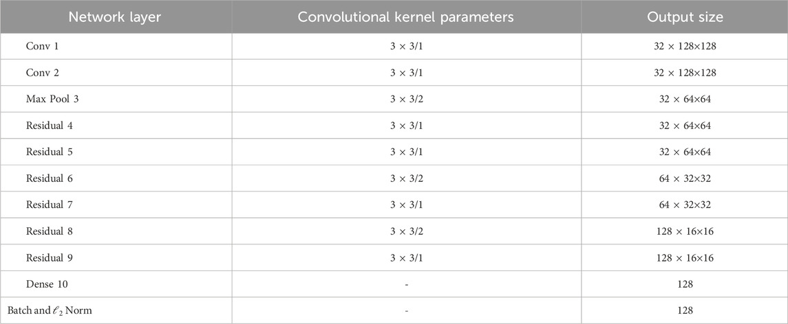
TABLE 3. Adjusted reconstruction network.
3 Vehicle speed measurement
3.1 Model assumptions
All locations in road monitoring images can be mapped to the
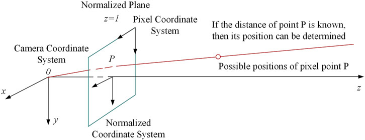
FIGURE 5. Pixel coordinate conversion diagram.
3.2 Model design and implementation
Based on the assumptions and establishment of the aforementioned speed model, the specific process of speed detection is implemented. Firstly, using the YOLO object detection algorithm, the coordinates of the top-left corner of the image detection box are obtained. By determining the length and width of the detection box, the coordinates of the center of the bottom edge of the box can be obtained. This ensures that the measured vehicle speed is closer to the actual speed. For every target vehicle in each frame of the video stream, a set of vector relations can be obtained, as shown in Eq. 10.
Here,
In This article, state estimation is performed using the popular methods of maximum likelihood estimation, maximum a posteriori estimation, and non-linear least squares, selecting the best estimation parameters based on the loss in state estimation.
(1) Maximum Likelihood Estimation
Maximum Likelihood Estimation (MLE) is an important and widely used method for estimating quantities. MLE explicitly uses a probability model with the goal of finding a system occurrence tree that can produce observed data with a high probability. MLE is a representative of a class of system occurrence tree reconstruction methods based entirely on statistics. Given a set of data, if we know it is randomly taken from a certain distribution, but we don't know the specific parameters of this distribution, that is, “the model is determined, but the parameters are unknown.” For example, we know the distribution is a normal distribution, but we don’t know the mean and variance; or it’s a binomial distribution, but we don’t know the mean. MLE can be used to estimate the parameters of the model. The objective of MLE is to find a set of parameters that maximize the probability of the model producing the observed data, as shown in Eq. 11.
Here,
To facilitate differentiation, the log is generally taken of the target. Therefore, optimizing the likelihood function is equivalent to optimizing the log-likelihood function, as shown in Eqs 13, 14.
(2) Maximum A Posteriori Estimation
In Bayesian statistics, Maximum A Posteriori (MAP) Estimation refers to the mode of the posterior probability distribution. MAP estimation is used to estimate the values of quantities that cannot be directly observed in experimental data. It is closely related to the classical method of Maximum Likelihood Estimation (MLE), but it uses an augmented optimization objective that further considers the prior probability distribution of the quantity being estimated. Therefore, MAP estimation can be seen as a regularized form of MLE, as shown in Eqs 15, 16.
Here,
(3) Non-Linear Least Squares
The Least Squares Method (also known as the Method of Least Squares) is a mathematical optimization technique. It finds the best function match for data by minimizing the sum of the squares of the errors. The Least Squares Method can be used to easily obtain unknown data, ensuring that the sum of the squares of the errors between these obtained data and the actual data is minimized. The Least Squares Method can also be used for curve fitting, and other optimization problems can be expressed using this method by minimizing energy or maximizing entropy. Using the Least Squares Method to estimate the mapping relationship, the mapping parameters are obtained, as shown in Eqs 17, 18.
Where
Then, the Gauss-Newton method is used to solve for ψ(x), as shown in Eq. 19:
For the sum of errors, we investigate the i term, also performing a second-order Taylor expansion, followed by differentiation. We first calculate its first-order derivative (gradient) and second-order derivative.
First-order derivative, as shown in Eqs 20, 21.
Where
Second-order derivative, as shown in Eq. 23.
Observing the result of the second-order derivative, the terms
Therefore, after the second-order expansion,
Similarly, by differentiating it and setting the derivative equal to zero, Eq. 26:
Let
3.3 Vehicle speed measurement
Through prior estimation,
Assuming a vehicle’s trajectory contains m frame trajectory points, meaning in the first m frames of the video, the vehicle’s speed between each adjacent pair of frames is
Therefore, the average driving speed of the target vehicle in the first m frames is as shown in Eq. 33. The detection of the target vehicle’s speed is achieved by calculating the average of the instantaneous speeds over multiple frames.
4 Model training and evaluation metrics selection
4.1 Experimental environment and model training
Experimental setup and hardware environment for the dataset: System Type: Windows 10 64-bit Operating System, Memory: 64GB, GPU: NVIDIA GeForce RTX3080ti, 24 GB Graphics Card. Software environment: The auxiliary environment includes CUDA V11.2, OpenCV4.5.3. This article tested different corresponding datasets for various traffic scenarios. The dataset established in This article comprises a total of 30,000 images, including a diverse collection from different scenes, angles, and times.
During training, 80% of the dataset was used for training, while 20% of the data was reserved for testing. Data augmentation was applied in this study, which involved random scaling, cropping, and arrangement of images using the Mosaic method. Random rotation (parameter set to 0.5), random exposure (parameter set to 1.5), and saturation (parameter set to 1.5) were employed to enrich the training data. The learning rate was initially set to 0.001, and the maximum number of training iterations was set to 50,000. To optimize model convergence, the learning rate was adjusted to 0.0005 after 40,000 iterations. The input images to the network were resized to a resolution of 416 × 416, and a batch size of 8 was used during training to ensure efficient network processing. The convergence of the model’s training loss and mAP (mean Average Precision) can be observed in Figure 6. It shows that the model converged around 3,000 iterations, and as the loss decreased, mAP also reached a high level.
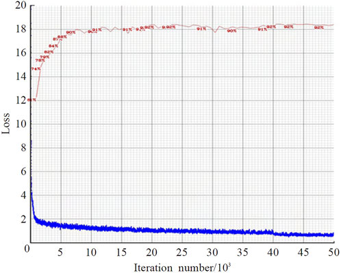
FIGURE 6. Model training loss convergence status.
Convolutional Neural Networks (CNNs) are capable of extracting key features from image objects. The detected objects are classified into three categories: Car, Truck, and Bus. The unique features of each class can be observed in Figure 7, where each class of object exhibits distinct characteristics within the convolutional network. These distinct features are used for classification and detection purposes.
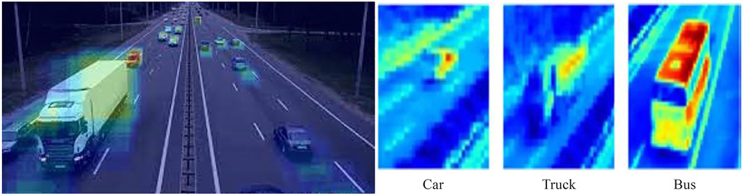
FIGURE 7. Classified target feature map.
4.2 Selection of evaluation metrics
To verify the effectiveness of the model’s detection, several typical metrics in the field of object detection and classification were selected for evaluation. For distracted driving behavior detection and classification, the focus is on detection precision and recall rate, as well as classification accuracy. Therefore, the model is evaluated using precision, recall, and F1_Score.
AP (Average Precision) is the average accuracy and a mainstream evaluation metric for object detection models. To correctly understand AP, it is necessary to use three concepts: Precision, Recall, and
Precision and Recall in object detection: Assuming a set of images containing several targets for detection, Precision represents the proportion of targets detected by the model that are actual target objects, while Recall represents the proportion of all real targets detected by the model. TP (True Positive) denotes samples correctly identified as positive, TN (True Negative) denotes samples correctly identified as negative, FP (False Positive) denotes samples incorrectly identified as positive, and FN (False Negative) denotes samples incorrectly identified as negative. The calculation of Precision and Recall values relies on the formulas shown in Eqs 35, 36.
After calculating values using the formula, a PR (Precision-Recall) curve can be plotted. The AP (Average Precision) is the mean of Precision values on the PR curve. To achieve more accurate results, the PR curve is smoothed, and the area under the smoothed curve is calculated using integral methods to determine the final AP value. The calculation formula is shown as Eq. 37.
The F1-Score, also known as the F1 measure, is a metric for classification problems, often used as the final metric in multi-class problems. It is the harmonic mean of precision and recall. For the F1-Score of a single category, the calculation formula is as shown in Eq. 38.
Subsequently, calculate the average value for all categories, denoted as F1. The calculation formula is shown in Eq. 39.
mAP (mean Average Precision) involves calculating the AP (Average Precision) for all categories and then computing the mean. The calculation formula is shown in Eq. 40.
5 Results and discussion
5.1 Evaluation of object detection model results
Based on the aforementioned evaluation metrics, the trained object detection models are tested and assessed using the test sets from the datasets. The algorithm shows good statistical accuracy for different vehicle types, with APs of Car, Bus, Truck being 93.58, 91.26, 90.05 respectively, mAP at 92.42, and F1_Score at 97. This is primarily due to the high visibility in tunnel and roadbed sections, where target features are more distinct, resulting in a more accurate model. Overall, the model’s detection accuracy for buses is lower than for other categories, mainly because the sample size for buses is significantly smaller than for other categories. However, with a mean Average Precision (mAP) exceeding 90%, it demonstrates that the proposed model is reliable and fully applicable to highway scenarios.
5.2 Evaluation of speed estimation results
5.2.1 Selection of optimal fitting model
Based on the data distribution, This article selects 7 video points for fitting analysis with 7 sets of linear and nonlinear data. This curve relationship is not intuitively obvious but requires statistical testing. The optimal fitting model is chosen by comparing the degree of fit and its significance. The Akaike Information Criterion (AIC) and Bayesian Information Criterion (BIC) are two commonly used indicators for assessing model fitness, with smaller values indicating a better-fitting model. Therefore, before selecting a model, it is necessary to assess the AIC and BIC values for each model, including dependent and independent variables. Additionally, the goodness of fit
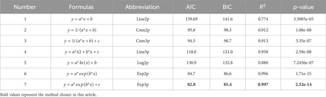
TABLE 4. Fitting model results.
From Table 4, it is evident that apart from linear fitting, the goodness of fit
To obtain the best fitting parameters for

TABLE 5. Parameter estimation results.
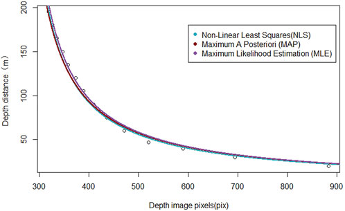
FIGURE 8. Parameter estimation results.
From the above table, it is clear that for the
5.2.2 Speed estimation results
To evaluate the measurement results of the speed estimation method, based on radar and video multi-sensor fusion technology, the results measured by millimeter-wave radar are taken as the true speed values. The verification experiment was conducted in the Shimen Tunnel on the Hanping Expressway in Shaanxi China, where radar and video integration devices were installed at 150-m intervals, totaling seven units, to achieve holographic perception of traffic flow states within a 1050-m range, obtaining detailed information on coordinates, lane positions, and speeds for different lanes and vehicle types. Vehicle speeds detected by millimeter-wave radar and video were extracted using timestamps and target IDs. The comparison between the measured results and the true speed values, along with the overall experimental results and performance analysis, are shown in Table 6.
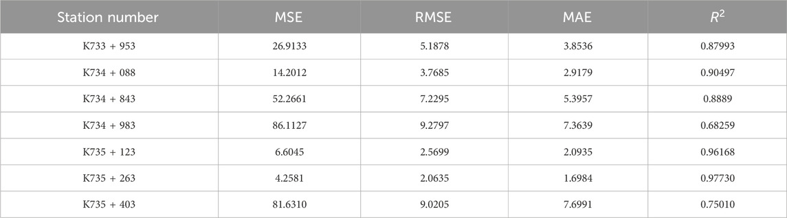
TABLE 6. Overall speed measurement results and performance analysis.
From Table 6, it is observed that the vehicle speed measurement method based on video, as discussed in This article, shows relatively good performance in scenarios with high overall speeds on highways. The minimum root mean square error is 2.0635, and the maximum is 9.2797. The main reasons for the larger deviation between the measured speeds and the actual values are environmental conditions, such as lighting and line shape. The coefficient of determination ranges from a minimum of 0.68259 to a maximum of 0.97730. The variation in the goodness of fit is for the same reasons as the minimum mean square error. Additionally, to further evaluate the speed tracking performance of this method, the vehicle speed measurement data from 7 video locations are manually divided into Front section, Middle section, Back section, and End section, for a comprehensive analysis of the overall tracking effect in these four segments, as seen in Figure 9.
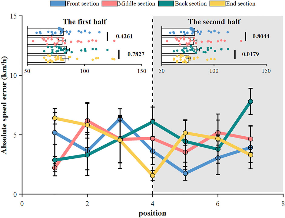
FIGURE 9. Analysis of speed tracking effect.
As depicted in Figure 9, the effective measurement distance of this method is around 140 m, with the absolute speed error generally within 1–8 km/h, meeting the accuracy requirements for speed measurement. This method has certain advantages in distance detection, especially in tunnel scenarios, where a camera spacing of 150 m allows for continuous tracking of vehicle trajectories and speeds based on video. For further analysis of speed tracking differences within the 150 m detection range, it's divided into The first half and The second half. The first half data shows a minimum significance level of 0.4261, indicating small differences in speed tracking, reflecting stable tracking performance. The second half data has a minimum significance level of 0.0179, indicating some fluctuations in speed in the End section of The second half, but the absolute speed error still shows good precision.
6 Conclusion
This article proposes an improved YOLOv5s + DeepSORT vehicle speed measurement algorithm for surveillance videos in highway scenarios, capable of vehicle target detection and continuous speed tracking without camera prior parameters and calibration. The main conclusions are as follows:
(1) The introduction of the Swin Transformer Block module improves the model’s ability to capture local areas of interest, effectively increasing the detector’s accuracy; using
(2) A calibration algorithm for traffic monitoring scenarios was proposed, which uses known reference points such as the image’s centerline and contour marks. It applies Maximum Likelihood Estimation, Maximum A Posteriori Estimation, and Non-linear Least Squares method for the conversion between image pixel coordinates and actual coordinates. The parameter estimation showed good results, with Maximum Likelihood Estimation being the best, and AIC, BIC,
(3) The vehicle speed measurement is achieved by calculating the average of instantaneous speeds over multiple frames. This method’s effective measurement distance is about 140m, with an absolute speed error generally within 1–8 km/h, meeting the accuracy requirements for speed measurement. It has certain advantages in distance detection, especially in tunnel scenarios where a camera spacing of 150 m allows for continuous tracking of vehicle trajectories and speeds based on video.
(4) However, during experiments, it was found that vehicle speed accuracy is influenced by road geometry, environmental conditions, lighting, resolution, etc., These can be mitigated through image enhancement optimization algorithms or by increasing video resolution, thus achieving more accurate vehicle speed measurements, which help regulatory bodies more effectively control speeds on the roads, reducing instances of speeding and thereby decreasing traffic accidents, enhancing road safety. Additionally, with the rapid development of multi-sensor fusion technology, the integration of video and millimeter-wave radar detection results can complement each other, providing technical support for active traffic safety management on highways.
Data availability statement
The original contributions presented in the study are included in the article/Supplementary material, further inquiries can be directed to the corresponding author.
Author contributions
ZL: Conceptualization, Methodology, Writing–original draft. YB: Funding acquisition, Writing–original draft. XY: Project administration, Resources, Writing–review and editing. YL: Investigation, Writing–review and editing. SY: Software, Writing–review and editing. MW: Funding acquisition, Project administration, Writing–review and editing. QY: Data curation, Writing–review and editing.
Funding
The author(s) declare financial support was received for the research, authorship, and/or publication of this article. This research was supported by the National Natural Science Foundation of China (52208424); the Natural Science Foundation of Chongqing (2022NSCQ-MSX1939); Chongqing Municipal Education Commission Foundation (KJQN202300728); Chongqing Talent Innovation Leading Talent Project (CQYC20210301505); The Key Research and Development Program of Guangxi, China, (Grant No. AB21196034).
Acknowledgments
The authors would like to thank the support of their colleagues in the Research and Development Center of Transport Industry of Self-driving Technology.
Conflict of interest
Authors ZL, XY, SY, MW, and QY were employed by China Merchants Chongqing Communications Research and Design Institute Co., Ltd.
The remaining authors declare that the research was conducted in the absence of any commercial or financial relationships that could be construed as a potential conflict of interest.
Publisher’s note
All claims expressed in this article are solely those of the authors and do not necessarily represent those of their affiliated organizations, or those of the publisher, the editors and the reviewers. Any product that may be evaluated in this article, or claim that may be made by its manufacturer, is not guaranteed or endorsed by the publisher.
References
1. Wan Y, Huang Y, Buckles B. Camera calibration and vehicle tracking: highway traffic video analytics. Transp Res C Emerg Technol (2014) 44:202–13. doi:10.1016/j.trc.2014.02.018
2. Karoń G, Mikulski J. Selected problems of transport modelling with ITS services impact on travel behavior of users. In: 2017 15th International Conference on ITS Telecommunications (ITST); 29-31 May 2017; Warsaw, Poland. IEEE (2017). p. 1–7. doi:10.1109/ITST.2017.7972231
3. Wang Y, Yu C, Hou J, Chu S, Zhang Y, Zhu Y. ARIMA model and few-shot learning for vehicle speed time series analysis and prediction. Comput Intell Neurosci (2022) 2022:1–9. doi:10.1155/2022/2526821
4. Jia S, Peng H, Liu S. Urban traffic state estimation considering resident travel characteristics and road network capacity. J Transportation Syst Eng Inf Tech (2011) 11:81–5. doi:10.1016/S1570-6672(10)60142-0
5. Javadi S, Dahl M, Pettersson MI. Vehicle speed measurement model for video-based systems. Comput Electr Eng (2019) 76:238–48. doi:10.1016/j.compeleceng.2019.04.001
6. Dahl M, Javadi S. Analytical modeling for a video-based vehicle speed measurement framework. Sensors (Switzerland) (2020) 20(1):160. doi:10.3390/s20010160
7. Khan A, Sarker DMSZ, Rayamajhi S. Speed estimation of vehicle in intelligent traffic surveillance system using video image processing. Int J Sci Eng Res (2014) 5(12):1384–90. doi:10.14299/ijser.2014.12.003
8. Wicaksono DW, Setiyono B. Speed estimation on moving vehicle based on digital image processing. Int J Comput Sci Appl Math (2017) 3(1):21–6. doi:10.12962/j24775401.v3i1.2117
9. Lu S, Wang Y, Song H. A high accurate vehicle speed estimation method. Soft Comput (2020) 24:1283–91. doi:10.1007/s00500-019-03965-w
10. Liu C, Huynh DQ, Sun Y, Reynolds M, Atkinson S. A vision-based pipeline for vehicle counting, speed estimation, and classification. IEEE Trans Intell Transportation Syst (2021) 22:7547–60. doi:10.1109/TITS.2020.3004066
11. Bhardwaj R, Tummala GK, Ramalingam G, Ramjee R, Sinha P. AutoCalib: automatic traffic camera calibration at scale. ACM Trans Sen Netw (2018) 14(3-4):1–27. doi:10.1145/3199667
12. Qimin X, Xu L, Mingming W, Bin L, Xianghui S. A methodology of vehicle speed estimation based on optical flow. In: Proceedings of 2014 IEEE International Conference on Service Operations and Logistics, and Informatics; 08-10 October 2014; Qingdao, China. IEEE (2014). p. 33–7. doi:10.1109/SOLI.2014.6960689
13. Schoepflin TN, Dailey DJ. Dynamic camera calibration of roadside traffic management cameras for vehicle speed estimation. IEEE Trans Intell Transportation Syst (2003) 4:90–8. doi:10.1109/TITS.2003.821213
14. Han J, Heo O, Park M, Kee S, Sunwoo M. Vehicle distance estimation using a mono-camera for FCW/AEB systems. Int J Automotive Tech (2016) 17:483–91. doi:10.1007/s12239-016-0050-9
15. Sochor J, Juranek R, Spanhel J, Marsik L, Siroky A, Herout A, et al. Comprehensive data set for automatic single camera visual speed measurement. IEEE Trans Intell Transportation Syst (2019) 20:1633–43. doi:10.1109/TITS.2018.2825609
16. Lin H-Y, Li K-J, Chang C-H. Vehicle speed detection from a single motion blurred image. Image Vis Comput (2008) 26:1327–37. doi:10.1016/j.imavis.2007.04.004
17. Celik T, Kusetogullari H. Solar-powered automated road surveillance system for speed violation detection. IEEE Trans Ind Elect (2010) 57:3216–27. doi:10.1109/TIE.2009.2038395
18. Nguyen TT, Pham XD, Song JH, Jin S, Kim D, Jeon JW. Compensating background for noise due to camera vibration in uncalibrated-camera-based vehicle speed measurement system. IEEE Trans Veh Technol (2011) 60:30–43. doi:10.1109/TVT.2010.2096832
19. Eslami H, Raie AA, Faez K. Precise vehicle speed measurement based on a hierarchical homographic transform estimation for law enforcement applications. IEICE Trans Inf Syst (2016) E99.D:1635–44. doi:10.1587/transinf.2015EDP7371
20. Famouri M, Azimifar Z, Wong A. A novel motion plane-based approach to vehicle speed estimation. IEEE Trans Intell Transportation Syst (2019) 20:1237–46. doi:10.1109/TITS.2018.2847224
21. Li J, Chen S, Zhang F, Li E, Yang T, Lu Z. An adaptive framework for multi-vehicle ground speed estimation in airborne videos. Remote Sens (Basel) (2019) 11:1241. doi:10.3390/rs11101241
22. Koyuncu H, Koyuncu B. Vehicle Speed detection by using Camera and image processing software. Int J Eng Sci (Ghaziabad) (2018) 7:64–72. doi:10.9790/1813-0709036472
23. Kim J-H, Oh W-T, Choi J-H, Park J-C. Reliability verification of vehicle speed estimate method in forensic videos. Forensic Sci Int (2018) 287:195–206. doi:10.1016/j.forsciint.2018.04.002
24. Sochor J, Juránek R, Herout A. Traffic surveillance camera calibration by 3D model bounding box alignment for accurate vehicle speed measurement. Computer Vis Image Understanding (2017) 161:87–98. doi:10.1016/j.cviu.2017.05.015
25. Palubinskas G, Kurz F, Reinartz P. Model based traffic congestion detection in optical remote sensing imagery. Eur Transport Res Rev (2010) 2:85–92. doi:10.1007/s12544-010-0028-z
26. Doǧan S, Temiz MS, Külür S. Real time speed estimation of moving vehicles from side view images from an uncalibrated video camera. Sensors (2010) 10(5):4805–24. doi:10.3390/s100504805
27. Li S, Yu H, Zhang J, Yang K, Bin R. Video-based traffic data collection system for multiple vehicle types. IET Intell Transport Syst (2014) 8:164–74. doi:10.1049/iet-its.2012.0099
28. Jeyabharathi D, Dejey DD. Vehicle tracking and speed measurement system (VTSM) based on novel feature descriptor: diagonal hexadecimal pattern (DHP). J Vis Commun Image Represent (2016) 40:816–30. doi:10.1016/j.jvcir.2016.08.011
29. Agrawal SC, Tripathi RK. An image processing based method for vehicle speed estimation. Int J Scientific Tech Res (2020) 9:1241–6.
30. Biswas D, Su H, Wang C, Stevanovic A. Speed estimation of multiple moving objects from a moving UAV platform. ISPRS Int J Geoinf (2019) 8(6):259. doi:10.3390/ijgi8060259
31. Lee J, Roh S, Shin J, Sohn K. Image-based learning to measure the space mean speed on a stretch of road without the need to tag images with labels. Sensors (Switzerland) (2019) 19:1227. doi:10.3390/s19051227
32. Dong H, Wen M, Yang Z. Vehicle speed estimation based on 3D ConvNets and non-local blocks. Future Internet (2019) 11(6):123. doi:10.3390/fi11060123
33. Luvizon DC, Nassu BT, Minetto R. A video-based system for vehicle speed measurement in urban roadways. IEEE Trans Intell Transportation Syst (2017) 18:1–12. doi:10.1109/TITS.2016.2606369
34. Yang L, Li M, Song X, Xiong Z, Hou C, Qu B. Vehicle speed measurement based on binocular stereovision system. IEEE Access (2019) 7:106628–41. doi:10.1109/ACCESS.2019.2932120
35. Blankenship K, Diamantas S. Detection, tracking, and speed estimation of vehicles: a homography-based approach. IMPROVE (2022) 1:211–8. doi:10.5220/0011093600003209
36. Fernández Llorca D, Hernández Martínez A, García Daza I. Vision-based vehicle speed estimation: a survey. IET Intell Transport Syst (2021) 15:987–1005. doi:10.1049/itr2.12079
37. Kim HJ. Vehicle detection and speed estimation for automated traffic surveillance systems at nighttime. Tehnicki Vjesnik (2019) 26:091448. doi:10.17559/TV-20170827091448
38. Ashraf MH, Jabeen F, Alghamdi H, Zia MS, Almutairi M. HVD-net: a hybrid vehicle detection network for vision-based vehicle tracking and speed estimation. J King Saud Univ - Comp Inf Sci (2023) 35:101657. doi:10.1016/j.jksuci.2023.101657
39. Pal SK, Pramanik A, Maiti J, Mitra P. Deep learning in multi-object detection and tracking: state of the art. Appl Intelligence (2021) 51:6400–29. doi:10.1007/s10489-021-02293-7
40. Jiao L, Zhang F, Liu F, Yang S, Li L, Feng Z, et al. A survey of deep learning-based object detection. IEEE Access (2019) 7:128837–68. doi:10.1109/ACCESS.2019.2939201
41. Khosravi H, Dehkordi RA, Ahmadyfard A. Vehicle speed and dimensions estimation using on-road cameras by identifying popular vehicles. Scientia Iranica (2022) 29. doi:10.24200/sci.2020.55331.4174
42. Huang L, Zhe T, Wu J, Wu Q, Pei C, Chen D. Robust inter-vehicle distance estimation method based on monocular vision. IEEE Access (2019) 7:46059–70. doi:10.1109/ACCESS.2019.2907984
43. Jamshidnejad A, De Schutter B. Estimation of the generalised average traffic speed based on microscopic measurements. Transportmetrica A: Transport Sci (2015) 11:525–46. doi:10.1080/23249935.2015.1026957
44. Sarkar NC, Bhaskar A, Zheng Z, Miska MP. Microscopic modelling of area-based heterogeneous traffic flow: area selection and vehicle movement. Transp Res Part C Emerg Technol (2020) 111:373–96. doi:10.1016/j.trc.2019.12.013
45. Appathurai A, Sundarasekar R, Raja C, Alex EJ, Palagan CA, Nithya A. An efficient optimal neural network-based moving vehicle detection in traffic video surveillance system. Circuits Syst Signal Process (2020) 39:734–56. doi:10.1007/s00034-019-01224-9
46. Liu Z, Lin Y, Cao Y, Hu H, Wei Y, Zhang Z, et al. Swin transformer: hierarchical vision transformer using shifted windows. Proc IEEE Int Conf Comp Vis (2021) 10012–22. doi:10.1109/ICCV48922.2021.00986
47. Zhang Q, Zhang M, Chen T, Sun Z, Ma Y, Yu B. Recent advances in convolutional neural network acceleration. Neurocomputing (2019) 323:37–51. doi:10.1016/j.neucom.2018.09.038
48. Bewley A, Ge Z, Ott L, Ramos F, Upcroft B. Simple online and realtime tracking. In: Proceedings - International Conference on Image Processing, ICIP; 17-20 September 2017; Beijing, China. IEEE (2016). p. 3464–8. doi:10.1109/ICIP.2016.7533003
49. Wojke N, Bewley A, Paulus D. Simple online and realtime tracking with a deep association metric. In: Proceedings - International Conference on Image Processing, ICIP; 17-20 September 2017; Beijing, China. IEEE (2017). p. 3645–9. doi:10.1109/ICIP.2017.8296962
50. Liu X, Liu W, Mei T, Ma H. A deep learning-based approach to progressive vehicle re-identification for urban surveillance. In: Lecture notes in computer science including subseries lecture notes in artificial intelligence and lecture notes in bioinformatics. Berlin, Germany: Spinger (2016). p. 869–84. doi:10.1007/978-3-319-46475-6_53
Keywords: YOLOv5S, Deep SORT, swin transformer, vehicle speed, traffic monitoring
Citation: Luo Z, Bi Y, Yang X, Li Y, Yu S, Wu M and Ye Q (2024) Enhanced YOLOv5s + DeepSORT method for highway vehicle speed detection and multi-sensor verification. Front. Phys. 12:1371320. doi: 10.3389/fphy.2024.1371320
Received: 16 January 2024; Accepted: 07 February 2024;
Published: 19 February 2024.
Edited by:
Guanqiu Qi, Buffalo State College, United StatesReviewed by:
Yunze Wang, Shijiazhuang Tiedao University, ChinaZhe Li, Hunan University, China
Ye Li, Central South University, China
Copyright © 2024 Luo, Bi, Yang, Li, Yu, Wu and Ye. This is an open-access article distributed under the terms of the Creative Commons Attribution License (CC BY). The use, distribution or reproduction in other forums is permitted, provided the original author(s) and the copyright owner(s) are credited and that the original publication in this journal is cited, in accordance with accepted academic practice. No use, distribution or reproduction is permitted which does not comply with these terms.
*Correspondence: Yanqiu Bi, Yml5YW5xaXVAY3FqdHUuZWR1LmNu