 L. Bonalumi1,2,3*
 E. Aymerich4
 E. Alessi2
 B. Cannas4
 A. Fanni4
 E. Lazzaro2
 S. Nowak2
 F. Pisano4
 G. Sias4
 C. Sozzi2 on behalf of JET Contributors† and WPTE team‡
- 1Department of Physics, Università degli Studi Milano Bicocca, Milan, Italy
- 2Istituto Scienza e Tecnologia per il Plasma (ISTPCNR), Milan, Italy
- 3DTT S.C. a r.l., Frascati, Italy
- 4Department of Electrical and Electronic Engineering, University of Cagliari, Cagliari, Italy
Introduction: This work explores the use of eXplainable artificial intelligence (XAI) to analyze a convolutional neural network (CNN) trained for disruption prediction in tokamak devices and fed with inputs composed of different physical quantities.
Methods: This work focuses on a reduced dataset containing disruptions that follow patterns which are distinguishable based on their impact on the electron temperature profile. Our objective is to demonstrate that the CNN, without explicit training for these specific mechanisms, has implicitly learned to differentiate between these two disruption paths. With this purpose, two XAI algorithms have been implemented: occlusion and saliency maps.
Results: The main outcome of this paper comes from the temperature profile analysis, which evaluates whether the CNN prioritizes the outer and inner regions.
Discussion: The result of this investigation reveals a consistent shift in the CNN’s output sensitivity depending on whether the inner or outer part of the temperature profile is perturbed, reflecting the underlying physical phenomena occurring in the plasma.
1 Introduction
Tokamak facilities rely on a combination of magnetic fields to confine the plasma. An important role is played by the magnetic field generated by a net current toroidally flowing in the plasma. To achieve efficient energy production in a fusion reactor, the plasma must be maintained for a sufficient amount of time that is much larger than the characteristic energy confinement time. The plasma is sensitive over different spatial and time scales to perturbations that can give rise to instabilities that destroy the magnetic configuration on a very small timescale. These phenomena, called disruptions, cause a sudden interruption of the plasma current that, in turn, induces strong electromagnetic forces in the metallic vessel and in the surrounding structures. Furthermore, the disruption process generates non-thermal relativistic electrons, called runaway electrons, that can damage the first wall of the machine. Due to the intrinsic non-linearity of the phenomena involved in a disruption, it is difficult to model the interactions that lead to the termination of the plasma discharge; however, it is possible to study processes that precede a disruption to identify and avoid disruptions before they happen. [1] performed a complete survey over a database of JET disruptions, identifying the chains of events, such as human errors in pulse management, MHD instabilities, like internal kink modes, or most importantly, neoclassical tearing modes (NTMs). In metallic wall machines, it is possible to identify the chain of events [2] related to the ingress of impurities or loss of density control, which determines the onset of an NTM and leads to disruption. Due to its fast, non-linear nature and the wide range of phenomena that can trigger a disruption, it is difficult to set up a system that is accurately able to predict and avoid a disruption. Various studies have highlighted promising applications of deep learning in the field of nuclear fusion research [3–5]. The use of convolutional neural network (CNN) architectures has shown great potential for disruption prediction. This technique can be exploited to monitor phenomena that lead to disruption (e.g., the locked modes [6]) or trained specifically to predict disruptions both using raw data from a specific tokamak [7] or across multiple machines [8,9]. The use of deep CNNs proves to be especially well-suited for the analysis of plasma profiles. In [10,11], the authors proposed the use of a deep CNN for the early detection of disruptive events at JET, utilizing both images constructed from 1-D plasma profiles and 0-D time signals. The predictors exhibit high performance, also comparing them with those of other machine learning algorithms [12]. The use of CNNs allows learning relevant spatiotemporal information straight from 1-D plasma profiles, avoiding hand-engineered feature extraction procedures. The CNN from [10] is adopted in the present paper to showcase the ability of eXplainable AI (XAI) methods to interpret network prediction, and its architecture is detailed in Section 2. The spread of deep learning algorithms depends on the trust that the scientific community has in these tools. One of the main causes of skepticism is that it is not possible to provide an explanation, neither in the testing phase nor in the training phase, of why a neural network produces a certain output. This issue becomes even more important when dealing with algorithms that are responsible for preventing and mitigating disruptions. The eXplainable artificial intelligence algorithms aim at providing an interface between humans and AI, producing results that explain the behavior of the neural network in a comprehensible way to humans [13,14]. An XAI analysis is a very flexible tool that strongly depends on the algorithm used. Specific XAI algorithms can be built ad hoc on the given AI system, however there exist agnostic algorithms generally applicable independently on the kind of AI. When dealing with CNNs, XAI algorithms provide a visual explanation, by producing heatmaps related to the input image that highlight the most relevant part of the input in order to classify the image. This work aims at addressing the problem of explaining how a neural network classifies a disruption, trying to fill the knowledge gap between CNN prediction and physical insights/interpretations. The application of XAI algorithms to CNNs in the problem of disruption prediction offers three main advantages. The first advantage is that there must be consistency between the explanations offered by XAI and the physical models. This consistency is essential to assert that the algorithm is genuinely learning to predict disruptions. So an analysis showing that the reason why an algorithm predicts a disruption is the same as the physical models contributes to increasing the trustworthiness of the NN. The second reason is that XAI might be able to provide indications about which signals are more useful for prediction, suggesting how to improve the performance of the CNN itself. The third reason lies in the unveiling of the CNN’s prediction process, enabling the identification of novel data patterns that may have eluded conventional physical investigations. This, in turn, offers valuable insights for the development of new physical models. In this paper, we will start analyzing a CNN trained to distinguish between disruptive and non-disruptive input data frames and compare the results with the physical classification of the disruptions, comparing how the CNN handles different disruptive paths. In Section 2.1, the CNN and training and test database sets are explained. The database has been analyzed and reduced, distinguishing between discharges following the two different paths. Two XAI methods are introduced in Section 3. Section 4 reports the results provided by the two methods, and the results are discussed and compared in Section 5.
2 The architecture of the neural network
The increasing use of deep learning in research is driven by improved computer processing power, allowing for the analysis of large datasets. Deep neural networks, known for their high accuracy even without complex feature extraction of the input data, play a key role in this. In image processing, convolutional neural networks (CNNs) are widely favored for their effectiveness in handling complex image data. Supported by these significant capabilities, [10] proposed the use of CNNs for extracting spatiotemporal features from JET 1-D plasma profiles (density, temperature, and plasma radiation) by converting them into 2-D images. Particularly, density and electron temperature from high-resolution Thompson scattering (HRTS) are pre-processed to synchronize time scales and eliminate outliers. Furthermore, in reference to Figure 1, showcasing the HRTS’s 63 lines of sight in blue, lines from the 54th to the 63rd position were excluded because of their inclination to generate unreliable data due to the outboard position. Concerning plasma radiation, in Figure 1, the 24 channels of the JET bolometer horizontal camera are depicted in green. In addition, data from these chords undergo the pre-processing steps mentioned for HRTS data. Three spatiotemporal images are created, with each pixel representing the measurement at the corresponding line of sight and time sample. These images are vertically stacked and normalized based on the signal ranges in the training set, producing an ultimate image. Figure 2 reports two showcases referring to two JET pulses. The generated images present, in a top-to-bottom sequence, and density and temperature data from 54 lines of sight measured by the HRTS, along with radiation data from the 24 chords of the horizontal bolometer camera. In total, there are 132 channels, and the data are presented over time. The final image is segmented using an overlapping sliding window of 200 ms, yielding individual image slices of size 132 × 101. As the CNN operates as a supervised algorithm, we explicitly assigned labels to slices in the training dataset. Those belonging to regularly terminated discharges were labeled as “stable.” In contrast, for disruptive discharges, the “unstable” label was automatically assigned by detecting the pre-disruptive phase through the algorithm proposed in [15]. For balancing the two classes, the stable phases of disrupted pulses were not included in the network training set, and the overlap durations of the sliding window were different for regularly terminated and disrupted discharges. Conversely, during the testing phase, a 2-ms stride was used for all discharges, covering both regularly terminated and disrupted pulses. Leveraging these diagnostics, which often exhibit behaviors linked to the onset of destabilizing physical mechanisms like MHD precursors, a straightforward CNN disruption prediction model is first deployed. In addition to the aforementioned plasma profiles, [10] takes into account 0-D diagnostic signals commonly used in the literature, specifically internal inductance and locked mode signals, as inputs for the disruption predictor. The internal inductance is indeed a crucial parameter because it provides information about the current profile within the plasma and is known to be connected to the density limit [16]. A higher internal inductance suggests a more peaked current profile, concentrated toward the plasma core, while a lower internal inductance indicates a more distributed or flat current profile. Moreover, at JET, mode locking indicates when a rotating (neoclassical) tearing mode locks with the external wall, which is closely followed by the disruption typically manifesting in the later stages of the disruptive process. JET provides a real-time mode locking signal. In [10], this signal has been normalized by the plasma current, as already done for disruption mitigation purposes. The normalized locked mode signal contributes significantly to the successful prediction of faster disruptions. The CNN architecture shown in Figure 3 comprises a series of interconnected convolutional (CU) and pooling (P) blocks, linked by a non-linear activation layer with a ReLU function. These blocks filter the input image both vertically (along the spatial dimension) and horizontally (along the temporal dimension), extracting essential features. These resulting features are fed into a fully connected multilayer perceptron neural network (FC), where the final SoftMax layer determines the likelihood of the input image slice belonging to either a regularly terminated or a disrupted discharge. To incorporate the two 0-D signals, the CNN architecture underwent modifications by introducing them downstream of the initial filter block. It is noteworthy that the first filter block was initially trained exclusively with 1-D diagnostic data, and its weights were subsequently frozen. In a subsequent training phase, both the second convolutional block and the FC block were trained using all plasma parameters. Note that the network architecture enables the separation of the two dimensions, spatial and temporal. Specifically, the first two blocks (CU1 and Pmax) filter solely across the spatial direction, while the subsequent two (CU2 and Pavg) filter exclusively across time. This facilitates the seamless concatenation of the 0-D signals (li and MLnorm) with the image features processed by the initial convolutional and pooling blocks, thereby preserving temporal synchronization. Figure 3 illustrates the ultimate CNN architecture, as presented in [10], showcasing the dimensions of input features for various blocks. Meanwhile, Table 1 provides a comprehensive overview of the corresponding parameters. The vertical kernel size for the convolutional and pooling blocks was designed considering a few constraints: a kernel size equal to or larger than 24 would have been larger than the bolometer number of lines of sight, and a small size kernel would reduce the effect of the discontinuity between the stacked diagnostic images. The small kernel size (5 × 1) allows the network to still identify changes in the spatial dimension of the HRTS scattering profile. Regarding time filtering, a similar operation was performed. Due to the different time resolutions of the diagnostics used, the filter size has been chosen to mainly process the highest frequency signals (the bolometer data). To determine the pooling type, two networks were trained: one with only average pooling and another with only max-pooling. Analyzing their performances on both the training and validation sets, it was observed that average pooling exhibited lower performance compared to max-pooling. However, the max-pooling response proved to be overly sensitive to transient changes in the data time traces. Consequently, the max-pooling layer was retained for spatial processing (vertical pooling), while average pooling was chosen for temporal pooling (horizontal pooling). Testing of discharges that were not included in the training phase underscores the predictor’s applicability across diverse operational scenarios.
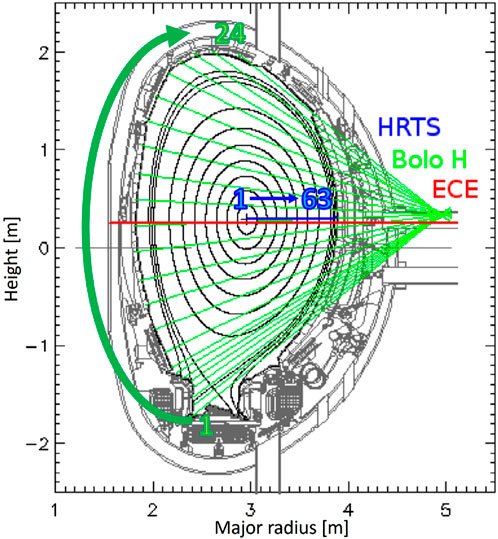
Figure 1. JET poloidal cross section: the 24 chords of the horizontal bolometer camera (in green) and the 63 lines of sight of the HRTS (in blue) are numbered according to the order in which they are taken to construct the image of the profiles as input to the CNN.
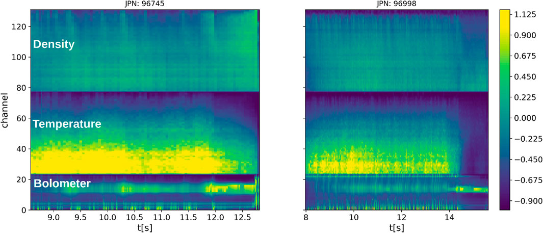
Figure 2. Two illustrative cases contained in the database. Left, edge cooling; right, temperature hollowing. The values on the color bar are expressed in terms of normalized unit
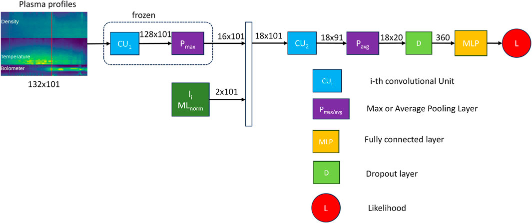
Figure 3. Final CNN architecture, where the internal inductance (li) and the normalized locked mode (MLnorm) serve as inputs to the second convolutional unit. These inputs are concatenated with the output image generated by the max-pooling layer.
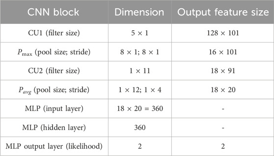
Table 1. CNN architecture.
In this paper, the described CNN predictor is considered to demonstrate the application of explainable AI, aiming to enhance the understanding and confidence in the decision-making process of the CNN predictor.
2.1 Database
The local balance of energy flowing into and out of a system determines its temperature profile. Impurities can break this balance by increasing the amount of energy that escapes as radiation. As a result, the temperature profile becomes susceptible to impurity penetration. The bolometer can provide an integrated measure of the radiative emission of the plasma. Strong radiation is associated with a loss of energy and, thus, a decrease in temperature. Usually, changes in the temperature profile are preceded by radiative losses measured using the bolometer. They depend on the distribution of impurity and density inside the plasma and can be categorized into two different ways: edge cooling (EC) and temperature hollowing (TH). Edge cooling is a collapse of the temperature profile at the edge, while temperature hollowing is a decrease in the central value of the temperature, often due to impurity accumulation on the plasma axis. A sketch of typical shapes of the temperature profile during edge cooling and temperature hollowing is depicted in Figure 4. These events are known to linearly destabilize the 2/1 mode [2], creating a magnetic island that rotates with the plasma. As it grows, the island experiences drag forces that tend to slow down its motion until the island locks onto the walls, leading to a disruption. We analyzed a database composed of 87 pulses, divided both in safe and disrupting modes, belonging to the train/test database of the neural network presented in Table 1 of [10]. Our database is composed of pulses that present a specific disruption path; in particular, the disrupting pulses are preceded by edge cooling (EC), temperature hollowing (TH), or a combination of TH, followed by EC (THEC). Table 2 shows the distribution in EC, TH, and THEC. For our purpose, the THEC pulses are considered pure TH. No indication regarding EC and TH has been provided to the CNN in the training phase. The input data are composed of radiation profiles of the horizontal chords of the bolometer diagnostic and the radial profile of the electron temperature from high-resolution Thompson scattering and the electron density. Data from the different channels are converted into images and vertically stacked. It is possible to define the time tEC/TH at which the EC/TH starts by introducing indexes related to the shape of the temperature profile [17], measured using the radiometer diagnostic, and defining the start of the event by introducing a conventional threshold. For every pulse of the database, tEC/TH has been measured. Two examples are shown in Figure 2. In temperature and density, higher channels correspond to a more external part of the profile. The temperature profile is obtained using Thompson scattering, which provides a measure of the electron temperature integrated along different lines of sight placed on the radial dimension. Examples of the different behavior for EC and TH are shown in Figure 2. The vertical red line represents the time at which EC/TH occurs. On the left side, an edge cooling case is presented. The collapse of the temperature at the edge is visible in the plot by the increase in the darker points in the region between channels 60 and 80, which represent the outer part of the profile. The edge cooling event starts with an increment in the radiated power, measured using the bolometer.
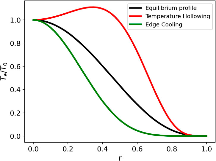
Figure 4. Sketch of typical shapes of the electron temperature profile after edge cooling (green line) and temperature hollowing (red line) events, compared with an equilibrium profile (black line).

Table 2. Summary of the different phenomena occurring in the pulses: edge cooling (EC), temperature hollowing (TH), and a temperature hollowing event followed by a combination of TH and EC (THEC). The safe pulses do not exhibit any of these phenomena.
The plot on the right represents the input image for the neural network in a temperature hollowing case. Here, the hollowing of the temperature profile on the plasma axis occurs at t = 54 s, and it is evident by looking at the channels between 20 and 40 that are part of the temperature profile on the plasma axis.
3 The XAI techniques
In general, an XAI algorithm is an additional layer of analysis built by the user on a given AI in order to produce an explanation of the output for a certain input. In this work, the XAI analysis is built over an existing CNN, described in Section 2, trained to predict disruptions. The input of the CNN is composed of physical quantities, and the aim of the XAI algorithm is to interpret which part of the input contributes the most to the classification of the image as disruptive or safe. This allows us to not only build a hierarchy of the most relevant physical quantities but also to understand which part of the profile of a certain physical input quantity matters the most. Various methods can be used to explore this issue. One approach is to analyze the sensitivity of the output when a perturbation is introduced at a certain point in the classification chain. This type of analysis, known as sensitivity analysis, produces a heatmap [18] that shows which part of the input has the greatest impact on the output. We can use this approach in two modes: agnostic and non-agnostic. In the agnostic mode, we do not delve into the behavior of the CNN’s internal components (weights and gradients). Instead, we directly perturb the input and analyze the resulting output changes. Conversely, the non-agnostic mode involves analyzing the output’s sensitivity with respect to the weights within the network’s hidden layers. In Sections 3.1 and 3.2, we will explain the methods adopted, briefly presenting an example of the output produced.
3.1 Occlusion
The most straightforward agnostic approach is the occlusion [19,20], where, as a perturbation, a constant value patch is applied in a certain part of the input, and the effect of the patch on the output is analyzed. We then interpret the fluctuation of the output as how important the part covered by the patch is for the classification. Each input image for the CNN is made up of 132 × 101 pixels, as reported in Section 2. Adopting the overlapping window approach to perform the occlusion is too computationally demanding because every time slice must be analyzed for every possible position of the patch. Therefore, the global input is divided into M non-overlapping temporal slices of dimension 132 × 101. To split the complete input into M sub-images, a zero padding p is introduced in order to ensure that Nt = p + 101 × M, where Nt is the time length of the pulse. A patch of dimensions W × H is introduced in every slice, producing a perturbed image which is the same as the original except for the area covered. The patch replaces the value of the pixel, with a constant value V. The patch is moved with a horizontal sh step and a vertical sv step. The width, height, and vertical and horizontal steps define the number of positions that the patch can assume to perturb the output. N perturbed sub-images Ioccl,k, with k = 1, …, k, are obtained, where every image contains the patch in a different position. The occluded input Ioccl,k is passed to the neural network, resulting in an output fNN(Ioccl,k) with
These are 132 × 101 matrices having the same dimensions (number of pixels) as the original image, where the non-zero elements have the same positions as the patch. The non-zero values of δk are the values of the fluctuation Δk. The matrix δk represents, for a given position of the patch, the pixels that, if occluded, produce the fluctuation Δk. The matrix ck is built so that the sum over all the possible k (positions of the patch) returns the number of times that a certain pixel (i, j) is covered by the patch:
Finally, we define the matrix δ as that matrix where every element (i, j) is the fluctuation Δk averaged over all the possible positions of the patch:
The matrix δ(i,j) represents the occlusion heatmap for a single sub-image 132 × 101. The occlusion depends on five free parameters related to the patch: the size (width W and height H), the value V, and the stride (horizontal sh and vertical sv). These parameters define how the input is perturbed by the occlusion method. By applying this method to all the slices, the occlusion produces a 132 × Nt output. Since the monodimensional signals are treated as distinct inputs, their occlusion is also performed independently. A patch of constant value V is applied to the 0-D signal region, leaving the 1-D signals unaffected. This patch is moved along the horizontal axis with step size sh, following the same algorithm as for the 1-D signals generating a 2 × Nt matrix. An example is provided in Figure 5: at the top, the heatmap for the 1-D signals is shown. Starting from the bottom, the image refers to the radiation, temperature, and density. The color intensity corresponds to the degree to which occluding a particular input feature affects the neural network’s output. A fluctuation of −1 indicates that occluding that input feature reduces the network’s output by 1, from 1 to 0. This matrix highlights the importance of each input feature for disruption classification. For visualization purposes, the fluctuation related to the signals is plotted in the plot in the middle, with the red line referring to li and the green line referring to the ML signal. The areas where the occlusion produces the strongest fluctuation are related to the bolometer and the central part of the temperature profile. The monodimensional signals, on the other hand, become important only in the transient phase, when the output of the neural network (black trace at the bottom) changes from stable to unstable or vice versa. The occlusion heatmap brought out an interesting behavior: the neural network seems to be sensitive mostly to the right part of the input. This behavior is shown in Figure 5 (top), where the areas highlighted in the bolometer are asymmetric, with a reverse d-shape.
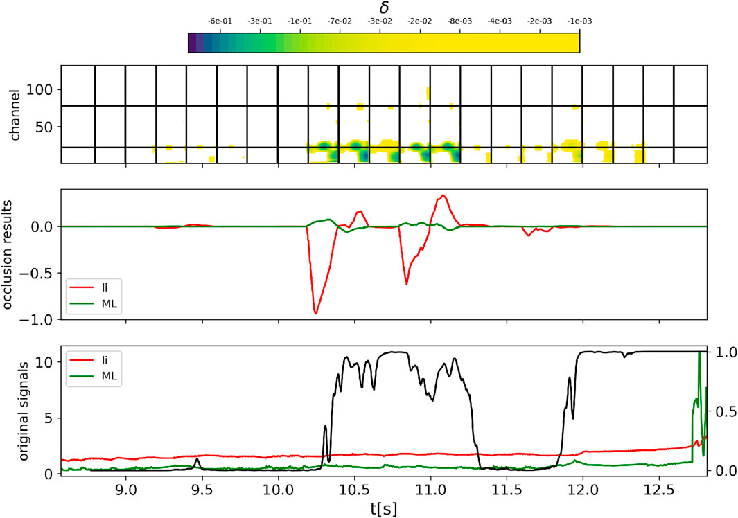
Figure 5. Occlusion analysis for the JPN 96745. The heatmap as a result of the occlusion technique for the 1-D signals (top) and the 0-D signals (middle). The red line refers to the fluctuation as a consequence of the occlusion of the internal inductance, while the green line is for the ML signal. The third plot (bottom) represents the output of the neural network (black line), the signal of the internal inductance (red line), and the ML signal (green line).
3.2 Saliency map
The previous method is coupled with a non-agnostic method to provide a more complete and general insight into the interpretation of the neural network. There is a wide variety of non-agnostic methods. Following [21], we define the saliency map as a matrix made up of the derivative of the output of the neural network backpropagated to every single pixel of the input. Due to the particular architecture of the neural network we are studying, the gradient of the output will be backpropagated until the second convolutional unit, as indicated in Figure 3. The second convolutional unit will produce as output a matrix A(α,β). A backpropagation to the input of the neural network is not possible as the network is interrupted to add the monodimensional signals before the second convolutional layer. The first convolutional layer reduces the image size, but the ratio between the distances remains the same. Therefore, we can understand which areas of the input the saliency map output refers to by simply rescaling it. The saliency map will have the same dimension as the network layer, where every element (α, β) will be the partial derivative of the output with respect to Aαβ(I) and is calculated as follows:
where we have introduced the operator max(•, 0), known as the ReLU (rectified linear unit), in order to filter out the negative values. The derivative is calculated with a guided backpropagation algorithm [22] that reduces the fluctuation of the gradient in the presence of the non-linear activation layer (e.g., the ReLu). The definition in Eq. (5) must be adapted to the structure of the neural network that we are trying to analyze. In this case, the global input
where k is the time of the right edge of the overlapping time window. For a certain time j, we have j ≤ k ≤ j + 101. Finally, we define the saliency map as
We averaged the single-frame saliency maps for all possible saliency maps that involve the pixel (i, j). The output of the saliency map is a heatmap 18 × Nt. An example is provided in Figure 6. Specifically, the channels at the bottom are related to the bolometer (0–3), then the temperature (4–10), and then the density (11–16), while at the top, there is the gradient with respect to the monodimensional signals (17–18). Figure 7 shows the function g of the saliency map for different phases of the pulse: a stable, a transient, and an unstable phase. The value of the function g in the different regimes is noteworthy: when the output of the neural network changes, passing from stable to unstable, the sensitivity of the output becomes larger by approximately three orders of magnitude. The saliency map shows that the most sensitive parts of the input are the radiation and the central part of the temperature, while the density seems to be of secondary importance and the monodimensional signals are only relevant close to the trigger of the alarm.
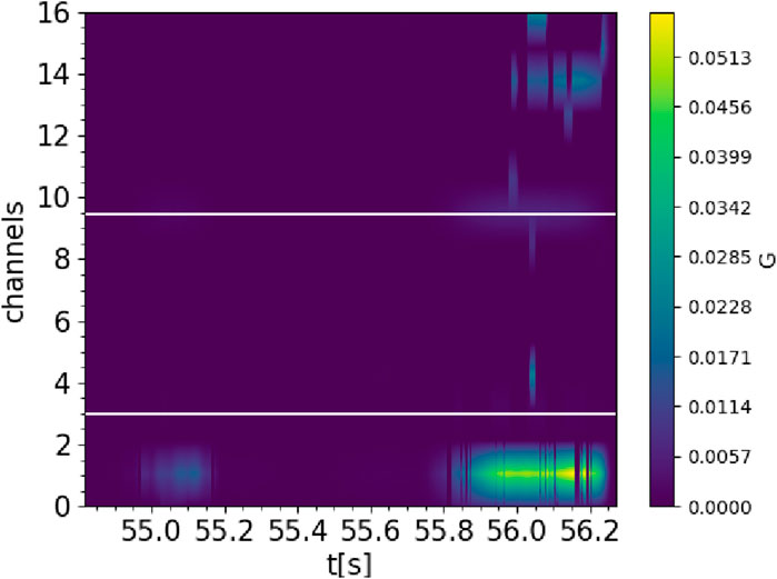
Figure 6. Saliency map for JPN 94966. The plot shows the matrix G, as defined in Eq. 7. Larger values of G are connected to larger values of the gradient of the output with respect to the output of the neuron in the second convolutional layer.
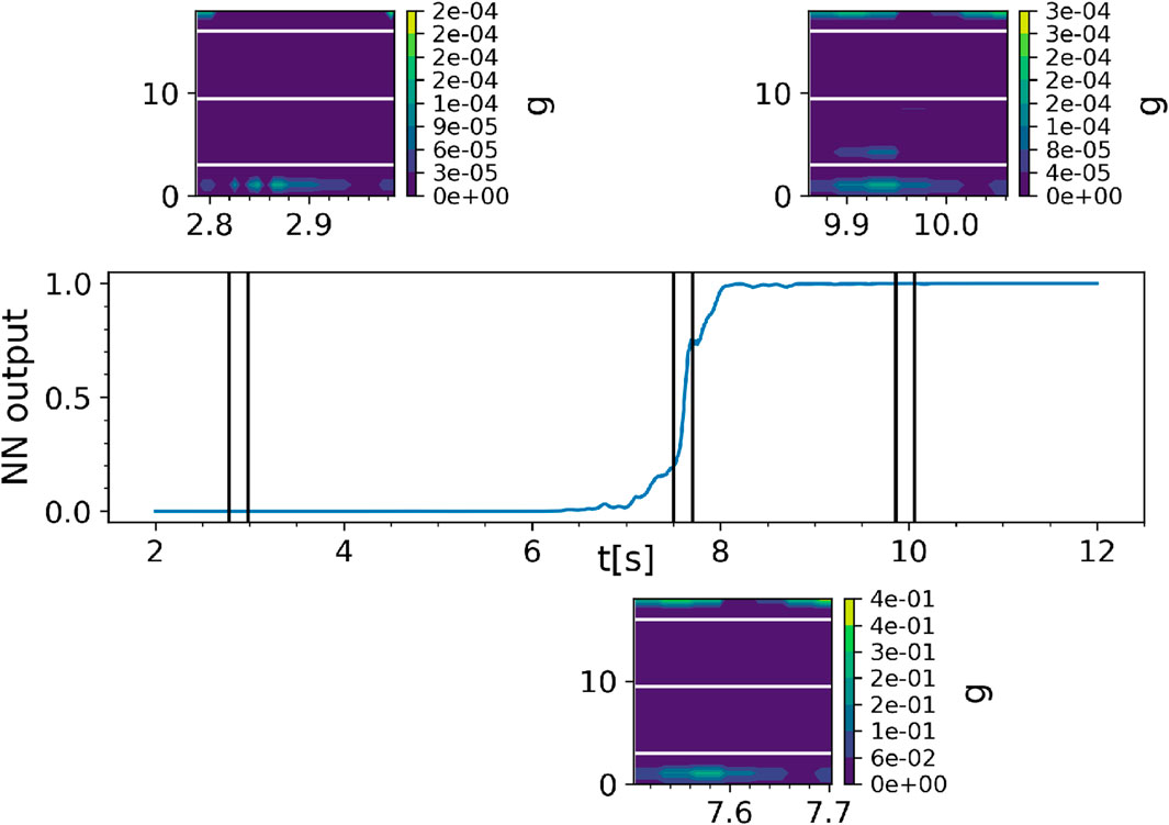
Figure 7. Example of the matrix g, as defined in Equation 5, for different times. The plot in the middle represents the output of the neural network. The images show saliency maps at different times.
4 Results
The sensitivity map and occlusion provide consistent results: there is a strong indication that the neural network relies mainly on the bolometer signal to make its predictions. The central part of the temperature profile is the second most important feature for the neural network, while 0-D signals play a role in the classification only near the alarm. The density seems to be of secondary importance for the disruption prediction. The saliency map tends to show a significant gradient in the bolometer even when there is no relevant signal in that area of the input. A comparison between different methods is shown in Figures 6, 8. The heatmaps turn on at the same moment, but in the saliency map, the area of the bolometer is much more important than the occlusion. The temperature is relevant for the occlusion, even though a peak in the inner part of the temperature profile can also be seen in the saliency map. In both heatmaps, there is an increase in sensitivity in the part connected to the density near the alarm, which anyway remains less relevant than the temperature and the radiation. The network does not recognize the change in the temperature profile that characterizes the EC/TH as the first event in the chain of phenomena that leads to disruption as the alarm is often triggered before the EC/TH event. This is the reason why the network is usually able to predict the disruption before the EC/TH event. However, it is interesting to understand whether the NN is sensitive to the change in the temperature that is physically responsible for triggering the instability, as described in Section 2.1. Since the occlusion technique includes several free parameters, it is suitable for analyzing individual discharges, but there is the risk of not being able to obtain a uniform procedure when comparing different discharges. For this reason, a local systematic analysis has been carried out using only the saliency map approach near the time of the EC/TH event, measured as reported in Section 2.1. Saliency maps are calculated close to the events of edge cooling and temperature hollowing. The maps are superimposed, and the gradient is averaged for every pixel. The result is shown in Figure 9. The plots show the aggregated heatmap for the EC (left) and TH (right) events. The two plots exhibit different behaviors: edge cooling highlights multiple areas (in the red circles) in the outer part of the profile where there are peaks in the gradient. On the other hand, temperature hollowing exhibits multiple peaks at the center of the profile, with a reduced value of the gradient at the edge. In addition, the plot for the EC event shows an important gradient at the center of the profile, but it has a more continuous behavior and lights up close to the peaks at the edge. Figure 9 shows that the gradient increase occurs in an interval of 200 ms before the EC/TH event. This is also confirmed in Figure 10, where the distribution of the temporal differences between the closest peak of the gradient and the time of EC/TH for all the analyzed pulses is plotted. The distribution peaks around t − tEC/TH = 0, confirming the strong correlation between the EC/TH event and the gradient increase. Furthermore, the distribution is strongly asymmetric, reflecting the tendency of the neural network to anticipate the EC/TH event. Figure 11 shows the position of every pulse of the database in the space composed by the average of the gradient in the inner and outer halves of the profile. The average gradient is calculated as the arithmetic mean of the elements of the matrix G around the time of the edge cooling/temperature hollowing event. The inner region refers to the temperature profile with r/a ∈ (0, 0.5), and the outer region refers to r ∈ (0.5, 1). Figure 11 shows that when analyzing edge cooling, the neural network tends to produce a heatmap with a non-zero gradient in the outer region, indicating that it maintains its focus on the edge in the presence of a physical phenomenon that affects that portion of the profile. On the other hand, temperature hollowing produces a heatmap with a zero average gradient on the edge, indicating that the neural network does not consider the outer region of the temperature profile to be important for classifying the disruption. Finally, we analyzed the safe pulses. Figure 12 shows the average of the sensitivity maps of all safe pulses around a reference time in the stable phase of discharge. The plot does not show any peaks in the gradient but rather a continuous area in the radiation and the 0-D signals. This indicates that the neural network does not focus on any particular phenomenon but maintains its attention on the radiation and the one-dimensional signals, waiting for some event that could represent a precursor to the disruption.
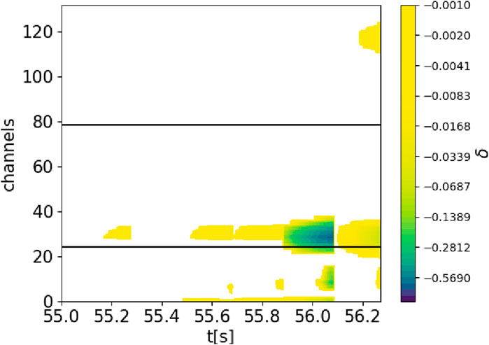
Figure 8. Occlusion analysis for the JPN 94966. The color bar represents the fluctuation δ, as defined in Eq. 4. The blue region corresponds to a stronger fluctuation as a consequence of the occlusion of that part of the input, which is interpreted as more importance given to that part of the input. White areas do not produce any fluctuation of the output. The colors are in a logarithmic scale.
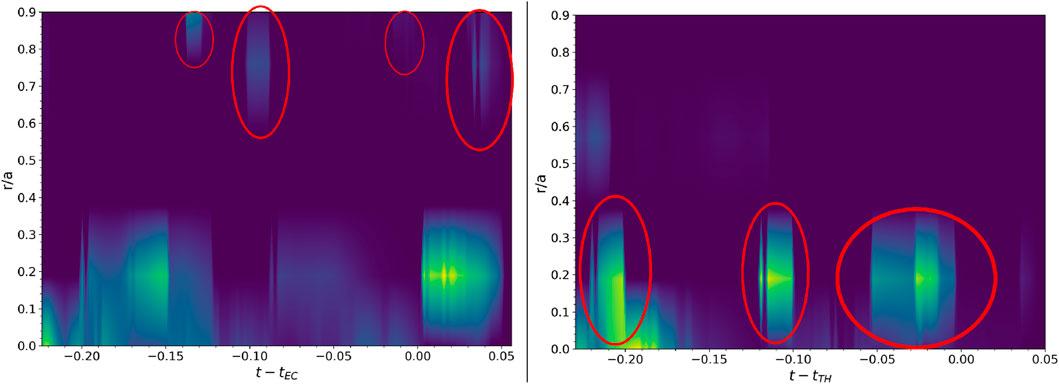
Figure 9. Plots of the average of the saliency maps of every pulse of the database for the edge cooling (left) and temperature hollowing (right) events.
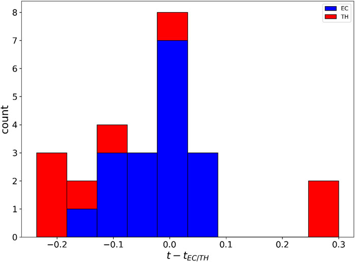
Figure 10. The temporal distance between the TH (red)/EC (blue) event and the closest peak in the gradient in the inner/outer part of the temperature profile.
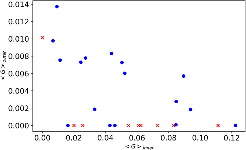
Figure 11. Plot of the points of the database in the space composed by the average of the gradient as defined in Eq. 7 in the inner and outer parts of the temperature profile.

Figure 12. Plot of the average saliency map for the safe pulses around a reference time during the stable phase.
5 Discussion of results
The XAI analyses provide insights about what the neural network considers important in the classification of a disruption, given a certain input. One of the objectives of this work is to understand if the neural network assigns importance to a class of phenomena (edge cooling and temperature hollowing) that involve multiple areas of the input and not only single points. For this reason, we decided to perform the analysis using sensitivity approaches that tend to produce results that highlight extensive areas rather than single pixels. Other approaches, such as decomposition, can, in principle, be used (an example is the layer-wise relevance propagation [23]). These methods assign a “relevance score” to every pixel of the input by decomposing the output of the network in series, generating heatmaps that pinpoint the most critical pixels, offering a granular view of the input’s impact on the final result. Between the algorithms following the sensitivity approach, we developed the saliency map and the occlusion. More complicated algorithms are available, although they are more suitable for larger CNNs. For example, the GRAD-CAM algorithm [24] involves summing the output of every feature map in a convolutional layer, weighted on an average pooling of the gradient of the final output with respect to the output of the feature map. However, this is thought to be applied on a CNN composed of one convolutional layer with many feature maps. The CNN we used is relatively simple, containing two convolutional layers with only one feature map, so GRAD-CAM would not provide any additional insights. The occlusion method is an agnostic method, easy to develop and interpret, but it intrinsically depends on different free parameters, such as the size of the occluded region. An in-depth analysis of the effect of occlusion parameters is beyond the scope of this work. The primary goal of using the two methods was to compare them and find a set of parameters, for which the results obtained are consistent with each other.
5.1 General results and comparison
As explained in Section 2, the CNN is fed with inputs composed of physical data measured by the diagnostics. At first, the analysis is performed over the entire input, taking into consideration all the quantities in the input. The comparison between the two methods (Figures 6, 8) allows us to identify the radiation as the most relevant part of the input for the classification. The central part of the temperature profile is also found to be particularly crucial. The monodimensional signals are important only close to the alarm time, and the density does not seem to be important in the classification. The comparison produces consistent results, even though some differences should be discussed. The occlusion method seems to produce maps that are more sensitive to the right part of an input image, as shown in Figure 5. Since the neural network is trained on temporally ordered input images, when a disruption occurs, its lines of evidence appear at first in the right part of the input. As a result, in the training phase, the CNN learns to be more sensitive to the right side of the input. This right-side bias is particularly evident in the occlusion technique because, in the saliency map approach, the final heatmap is the average of multiple heatmaps produced with the sliding window, so the effect eventually averages out. The saliency map can be applied systematically to the data but often produces biased results. In particular, the saliency map tends to have a strong gradient on the radiation, even when there is no significant signal. This could be because the CNN, in the training phase, adjusts its weights to give more importance to the radiation since it has learned that it is an important feature. This implies that the gradient of the radiation, when backpropagated, is stronger with respect to the gradient coming from other diagnostics. It also reflects in the XAI analysis as the gradient in the radiation part of the input is highlighted with respect to the gradient of the other diagnostics, even if no relevant signals are present in the input. So the second part of the analysis focuses specifically on the temperature profile.
5.2 Analysis of the temperature
The main result of this paper is that there is strong evidence that the neural network is able to identify edge cooling and temperature hollowing. This is shown in Figure 9, where the average of the gradient matrix G (as defined in Section 3.2), close to the EC/TH event, is shown for all the disruptions. This is also confirmed in Figure 10 and Figure 11. In the latter, it is also evident that the gradient’s average is greater in the inner region of the profile than in the outer. This confirms that, in general, the neural network places more emphasis on the temperature profile on the axis than on the edge. Furthermore, in Figure 11, there are five points that represent edge cooling, but the gradient in the outer region is zero. Figure 13 shows that the network gives the alarm close to the edge cooling (
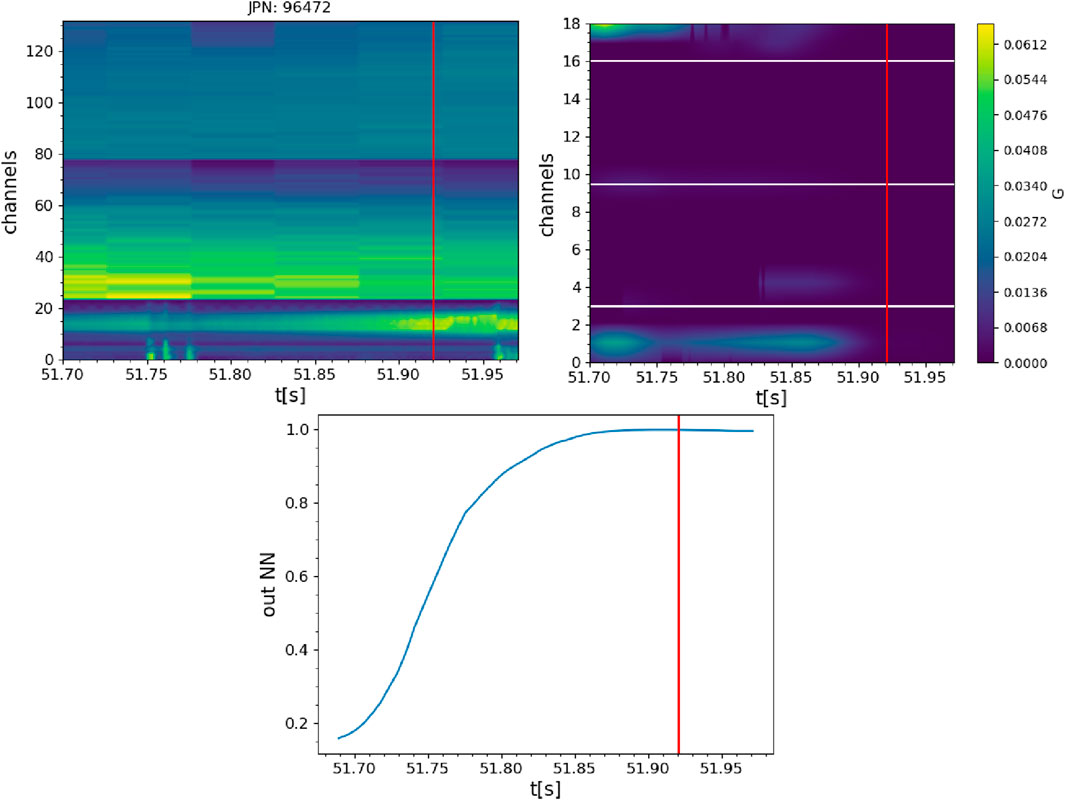
Figure 13. Plot shows an explanation for the behavior of the points in Figure 11. The vertical red line represents the time of the edge cooling. The top left plot represents the input image of the neural network. On the top right, there is the saliency map that corresponds to that input. At the bottom, there is the output of the neural network.
6 Conclusion
This work shows the potential of XAI analysis in explaining the output of a CNN trained for disruption prediction. Regarding disruptions having edge cooling and temperature hollowing as precursors, the CNN behaves consistently with what we know from physics, without providing any hint in the training phase. This could contribute to enhance the reliability of the neural network and promote its use in a disruption avoidance system. Furthermore, in principle, this could indicate that it is possible to investigate the physics by interpreting the way a neural network produces its output.
Data availability statement
The data analyzed in this study are subject to the following licenses/restrictions: EUROfusion GA (21) 35–3.4—Publication Rules Issue 2 14-July-2021 (Decision) + Grant Agreement 1010522200 Article 17: Communication, Dissemination, Open science, and Visibility. Requests to access these datasets should be directed to https://users.jetdata.eu/.
Author contributions
LB: writing–review and editing, writing–original draft, visualization, supervision, software, methodology, investigation, formal analysis, and conceptualization. EAy: writing–review and editing, validation, supervision, methodology, and data curation. EAl: writing–review and editing, validation, supervision, methodology, investigation, and conceptualization. BC: writing–review and editing, validation, supervision, and data curation. AF: writing–review and editing, supervision, methodology, and data curation. EL: writing–review and editing, validation, and supervision. SN: writing–review and editing and supervision. FP: writing–review and editing, validation, supervision, and data curation. GS: writing–review and editing, validation, supervision, methodology, investigation, and data curation. CS: writing–review and editing, validation, supervision, and project administration.
Funding
The author(s) declare that financial support was received for the research, authorship, and/or publication of this article. This work has been carried out within the framework of the EUROfusion Consortium, funded by the European Union via the Euratom Research and Training Program (grant agreement no. 101052200 EUROfusion).
Conflict of interest
Author LB is a PhD student supported by DTT S.C. a r.l.
The remaining authors declare that the research was conducted in the absence of any commercial or financial relationships that could be construed as a potential conflict of interest.
Publisher’s note
All claims expressed in this article are solely those of the authors and do not necessarily represent those of their affiliated organizations, or those of the publisher, the editors, and the reviewers. Any product that may be evaluated in this article, or claim that may be made by its manufacturer, is not guaranteed or endorsed by the publisher.
Author disclaimer
The views and opinions expressed are, however, those of the author(s) only and do not necessarily reflect those of the European Union or the European Commission. Neither the European Union nor the European Commission can be held responsible for them.
References
1. DeVries PC, Johnson MF, Alper B, Buratti P, Hender TC, Koslowski HR, et al. Survey of disruption causes at jet. Nucl Fusion (2011) 51:053018. doi:10.1088/0029-5515/51/5/053018
2. Pucella G, Buratti P, Giovannozzi E, Alessi E, Auriemma F, Brunetti D, et al. Onset of tearing modes in plasma termination on jet: the role of temperature hollowing and edge cooling. Nucl Fusion (2021) 61:046020. doi:10.1088/1741-4326/abe3c7
3. Pavone A, Merlo A, Kwak S, Svensson J. Machine learning and bayesian inference in nuclear fusion research: an overview. Plasma Phys Controlled Fusion (2023) 65:053001. doi:10.1088/1361-6587/acc60f
4. Farias G, Fabregas E, Dormido-Canto S, Vega J, Vergara S, Bencomo SD, et al. Applying deep learning for improving image classification in nuclear fusion devices. IEEE Access (2018) 6:72345–56. doi:10.1109/ACCESS.2018.2881832
5. Ferreira DR, Carvalho PJ, Fernandes H. Deep learning for plasma tomography and disruption prediction from bolometer data. IEEE Trans Plasma Sci (2020) 48:36–45. doi:10.1109/TPS.2019.2947304
6. Ferreira DR, Martins TA, Rodrigues P, Contributors JE. Explainable deep learning for the analysis of mhd spectrograms in nuclear fusion. Machine Learn Sci Technol (2022) 3:015015. doi:10.1088/2632-2153/ac44aa
7. Churchill RM, Tobias B, Zhu Y. Deep convolutional neural networks for multi-scale time-series classification and application to tokamak disruption prediction using raw, high temporal resolution diagnostic data. Phys Plasmas (2020) 27. doi:10.1063/1.5144458
8. Kates-Harbeck J, Svyatkovskiy A, Tang W. Predicting disruptive instabilities in controlled fusion plasmas through deep learning. Nature (2019) 568:526–31. doi:10.1038/s41586-019-1116-4
9. Zhu JX, Rea C, Granetz RS, Marmar ES, Sweeney R, Montes K, et al. Integrated deep learning framework for unstable event identification and disruption prediction of tokamak plasmas. Nucl Fusion (2023) 63:046009. doi:10.1088/1741-4326/acb803
10. Aymerich E, Sias G, Pisano F, Cannas B, Carcangiu S, Sozzi C, et al. Disruption prediction at jet through deep convolutional neural networks using spatiotemporal information from plasma profiles. Nucl Fusion (2022) 62:066005. doi:10.1088/1741-4326/ac525e
11. Aymerich E, Sias G, Pisano F, Cannas B, Fanni A, the JET-Contributors. Cnn disruption predictor at jet: early versus late data fusion approach. Fusion Eng Des (2023) 193:113668. doi:10.1016/j.fusengdes.2023.113668
12. Aymerich E, Cannas B, Pisano F, Sias G, Sozzi C, Stuart C, et al. Performance comparison of machine learning disruption predictors at jet. Appl Sci (Switzerland) (2023) 13:2006. doi:10.3390/app13032006
13. Gilpin LH, Bau D, Yuan BZ, Bajwa A, Specter M, Kagal L. Explaining explanations: an overview of interpretability of machine learning. In: 2018 IEEE 5th International Conference on Data Science and Advanced Analytics (DSAA); 01-03 October 2018; Turin, Italy (2018). p. 80–9. doi:10.1109/DSAA.2018.00018
14. Angelov PP, Soares EA, Jiang R, Arnold NI, Atkinson PM. Explainable artificial intelligence: an analytical review. WIREs Data Mining Knowledge Discov (2021) 11:e1424. doi:10.1002/widm.1424
15. Aymerich E, Fanni A, Sias G, Carcangiu S, Cannas B, Murari A, et al. A statistical approach for the automatic identification of the start of the chain of events leading to the disruptions at jet. Nucl Fusion (2021) 61:036013. doi:10.1088/1741-4326/abcb28
16. Snipes JA, Campbell DJ, Hugon M, Lomas PJ, Nave MF, Haynes PS, et al. Large amplitude quasi-stationary mhd modes in jet. Nucl Fusion (1988) 28:1085–97. doi:10.1088/0029-5515/28/6/010
17. Rossi R, Gelfusa M, Flanagan J, Murari A. Development of robust indicators for the identification of electron temperature profile anomalies and application to jet. Plasma Phys Controlled Fusion (2022) 64:045002. doi:10.1088/1361-6587/ac4d3b
18. Velden BHVD. Explainable ai: current status and future potential. Eur Radiol (2023) 34:1187–9. doi:10.1007/s00330-023-10121-4
20. Gohel P, Singh P, Mohanty M. Explainable AI: current status and future directions. CoRR abs/2107 (2021) 07045. doi:10.48550/arXiv.2107.07045
21. Simonyan K, Vedaldi A, Zisserman A. Deep inside convolutional networks: visualising image classification models and saliency maps (2014).
22. Springenberg JT, Dosovitskiy A, Brox T, Riedmiller M (2015). Striving for simplicity: the all convolutional net
23. Montavon G, Binder A, Lapuschkin S, Samek W, Müller K-R. Layer-wise relevance propagation: an overview. Cham: Springer International Publishing (2019). p. 193–209. doi:10.1007/978-3-030-28954-6_10
Keywords: nuclear fusion, disruptions, tokamak, JET, CNN, XAI, occlusion, saliency map
Citation: Bonalumi L, Aymerich E, Alessi E, Cannas B, Fanni A, Lazzaro E, Nowak S, Pisano F, Sias G and Sozzi C (2024) eXplainable artificial intelligence applied to algorithms for disruption prediction in tokamak devices. Front. Phys. 12:1359656. doi: 10.3389/fphy.2024.1359656
Received: 21 December 2023; Accepted: 01 April 2024;
Published: 14 May 2024.
Edited by:
Teddy Craciunescu, National Institute for Laser Plasma and Radiation Physics, RomaniaReviewed by:
Ralf Schneider, University of Greifswald, GermanyDragos Iustin Palade, National Institute for Laser Plasma and Radiation Physics, Romania
Gary Saavedra, Los Alamos National Laboratory (DOE), United States
Copyright © 2024 Bonalumi, Aymerich, Alessi, Cannas, Fanni, Lazzaro, Nowak, Pisano, Sias and Sozzi. This is an open-access article distributed under the terms of the Creative Commons Attribution License (CC BY). The use, distribution or reproduction in other forums is permitted, provided the original author(s) and the copyright owner(s) are credited and that the original publication in this journal is cited, in accordance with accepted academic practice. No use, distribution or reproduction is permitted which does not comply with these terms.
*Correspondence: L. Bonalumi, bHVjYS5ib25hbHVtaUBpc3RwLmNuci5pdA==
†See the author list of ‘Overview of JET results for optimizing ITER operation’ by J. Mailloux et al 2022 Nucl. Fusion 62 042026
‡See the author list of E. Joffrin et al. Nucl. Fusion, 29th FEC Proceeding (2023)