 Hunter Stephens
 Xinyi Li
 Yang Sheng
 Qiuwen Wu
 Yaorong Ge
 Q. Jackie Wu
- 1Department of Radiation Oncology, Duke University, Durham, NC, United States
- 2Department of Software and Information Systems, University of North Carolina at Charlotte, Charlotte, NC, United States
Head and neck (HN) cancers pose a difficult problem in the planning of intensity-modulated radiation therapy (IMRT) treatment. The primary tumor can be large and asymmetrical, and multiple organs at risk (OARs) with varying dose-sparing goals lie close to the target volume. Currently, there is no systematic way of automating the generation of IMRT plans, and the manual options face planning quality and long planning time challenges. In this article, we present a reinforcement learning (RL) model for the purposes of providing automated treatment planning to reduce clinical workflow time as well as providing a better starting point for human planners to modify and build upon. Several models with progressing complexity are presented, including the relevant plan dosimetry analysis and model interpretations of the resulting strategies learned by the auto-planning agent. Models were trained on a set of 40 patients and validated on a set of 20 patients. The presented models are shown to be consistent with the requirements of an RL model to be underpinned by a Markov decision process (MDP). In-depth interpretability of the models is presented by examination of the decision space using action hyperplanes. The auto-planning agent was able to generate plans with superior reduction in the mean dose of the left and right parotid glands by approximately 7 Gy
1 Introduction
The designing process of a radiation therapy treatment plan for head and neck (HN) cancers can be time-consuming. The proximity of critical organs to a usually large and asymmetric primary target volume (PTV) leads to numerous trade-offs between sparing adjacent organs at risk (OARs) and healthy tissue and delivering the prescribed radiation dosage to the tumor. These trade-offs are usually based on more complex dosimetric endpoints other than simply the minimum or maximum dose limits, in particular the mean or median dose for the parotid glands and oral cavity. The parotid glands are important to spare at the risk of severe xerostomia or inadequate salivary function. Complications from xerostomia include poor dental hygiene, oral infections, sleep disturbances, pain, and difficulty chewing and swallowing [1]. This must be considered as the target must be treated, but complications should be avoided for the long-term health of the patient. Radiobiological and post-treatment studies have shown that severe xerostomia can be avoided by limiting at least one of the glands’ mean dose to less than 20 Gy or the dose of both glands to less than 25 Gy [2]. Over dosing of the oral cavity can lead to severe complications or oral mucositis that can have a very strong, negative impact on the patient’s quality of life [3]. To avoid these side effects, Wang et al. [4] recommends that the oral cavity outside of the PTV should have a mean dose of less than 41.8 Gy, which is associated with a significant reduction in oral mucositis as compared to 58.8 Gy.
The highly conformal and sharp gradient distributions from intensity-modulated radiation therapy (IMRT) have been shown to have a significant improvement in parotid gland sparing over 3D conformal therapy [5–7]. This is due to the fact that modulation of the radiation fields can be optimized given a specific objective set by solving an inverse optimization problem based on the dose deposition matrices of the treatment field set. However, although parotid glands are anatomically symmetric, relative to each other, it is common for the parotid glands to not be symmetric about the PTV due to the irregularity of the defined target. It is possible for one parotid gland to be more proximal to the target and/or have a larger overlap volume. This leads to the difficulty in sparing the two parotids evenly. A more proximal gland may not be able to meet the dose objectives, while the other could have a more optimal dose distribution than prescribed. In this case, the dose objectives can be removed or relaxed from one gland to enhance the sparing of the other [8]. This is commonly referred to single-side versus bi-lateral sparing. It is usually determined by the physician by examining the spatial features of the parotid glands in relation to the PTV. While no particular protocol is used to determine single-side or bi-lateral sparing, there have been many methods developed to predict the possible sparing of OARs determined by anatomical features and past plans [7, 9–13]. Furthermore, it has been shown that the predicted median dose is suitable as a criterion for choosing single-sided or bi-lateral sparing [14].
Different PTVs in HN cancer often have several dose levels. The first is to a larger target volume that includes the entire region to be treated and is usually prescribed a dose of approximately 44 Gy. The second is to a smaller region within the large target region that will receive another boosted dose usually of approximately 26 Gy. Together, these two planning schemes create a volume with a prescription of 44 Gy and a prescription of 70 Gy to the smaller contained boosted region and are noted as the primary, boost, and plan sum, respectively. There are two primary strategies for achieving this: simultaneous integrated boost (IMRT-SIB) and sequential (IMRT-SEQ). IMRT-SIB achieves the treatment plan by treating the primary and boosted target simultaneously, while IMRT-SEQ treats them as two separate plans. Both methods have been shown to have similar survival rates [15], and thus for this study, IMRT-SEQ will be used as is consistent with our institutions’ current practice.
While this potential exists, the complex nature of the planning process coupled with the trial-and-error tuning of planning objectives results in a plan quality that is highly correlated to the planner’s experience [16]. This has led to a large influx of research into aiding this planning process using machine learning techniques [17]. One of the more seminal and important tools is knowledge-based planning (KBP), which aims to estimate certain aspects of a plan such as the dose distribution and dose–volume histograms (DVHs). This method has been widely used and studied [18–23]. Perhaps, the most optimistic application of machine learning to automatic planning can be found using reinforcement learning (RL), in which a machine seeks to mimic the decision processes of an expert planner. While in the nascent stages of development, RL has shown some promising results in modifying prostate plans where an intermediate plan was given as the input and an optimal strategy predicted [24, 25]. Again with prostate plans, automatic planning was shown to have success using deep reinforcement learning to modify plan parameters [26]. RL was also used for non-small-cell lung cancer; however, this application relied on a 3D dose prediction engine [27]. Neither of these applications seemed to demonstrate de novo plan creation and/or relied on methods with little to no interpretability. While deep learning methods have shown very positive and encouraging results, there is a lack of interpretability and sometimes a requirement of a large amount of data for the models to train properly. Another good and more relevant example of interpretable RL is found in the work done by Zhang et al. [28] in the development of an auto-planning agent for stereotactic body radiation therapy (SBRT) for pancreatic cancer. The action space used in this model consisted of increasing and decreasing the maximum or minimum dose values so that the state and action space could be easily interpreted. However, more often, objectives other than the minimum and maximum dose are used in planning, and a more robust action space is needed as is the case with HN cancers. At this time, there exists no technology for creating IMRT plans from scratch, which can handle the complexity of HN cancer treatment with multiple goals and provide an insight into the strategy used by the planning agent. Therefore, this work aims to explore the development and investigation of an RL model for the purposes of HN IMRT planning.
2 Methods
2.1 Model definitions and transition probabilities
RL can be modeled as a Markov decision process (MDP). An MDP is a 4-tuple,
•
•
•
•
•
Each of these will be defined for this model in the following sections. The following notation will be adopted. The state will be denoted by a vector,
The RL process can be described as the iterative interaction of an agent with an environment. The environment is defined by some current state observed by the agent. Ideally, this should include all the information available to the agent to make informed decisions. In the treatment planning process, a human planner mainly observes three objects of information. The first is the current dose distribution. Irrespective of the current plan configuration (beam settings, IMRT objectives, etc.), there is some resulting dose distribution. A human planner can observe the full distribution or the individual DVHs for OARs of interest. Most of this information is unnecessary or unprocessable for a human. Simply including all the information into the state vector would exponentially increase the model size, leading to an intractable problem. For instance, the entire dose distribution is defined at every point within a 3-D volume and can contain thousands of data points. Thus, in the proposed RL model, a dosimetric summary for each structure of interest will be included in the state definition. For the parotid glands and oral cavity, both the mean and median doses are included in the state, and for the PTV, the doses at 95% and 1% volume are included to summarize the target’s coverage and hotspot. These are included to ensure that the target is sufficiently treated (coverage) and that the dose is not too high (hotspot) to cause complications. The second piece of information is the current objective set for the plan. When deciding whether to move a planning objective for a structure, a human planner will take into consideration where the current objective is. If there is not much difference in the objective and the current dosimetry, then that objective could possibly be pushed further. The converse is true as well, in that a large difference between the objective and current dosimetric state could indicate that the objective movement would not have a large impact on the change of state. A third piece of information is the spatial features of the patient’s anatomy. The size and proximity of critical organs to the PTV play a large role in how well the organ can be spared. This would impact how much a human planner would need to decrease the dose for a particular organ. For example, if one of the parotids had a substantial overlap with the target, then getting the mean dose below 25 Gy would be quite difficult without substantially lessening the coverage of the target. For the purposes of the current study, the spatial features are not directly represented in the state definition. It is assumed that this information is inherently encoded into the dose deposition matrix as the deposition matrix is a function of the anatomy distribution. This can be reasoned from the fact that the optimization, which is driven by the dose deposition matrix, will have certain responses based on the spatial characteristics of the medium. The agent will be assumed to gain the spatial information from the response of the optimization. The environment state is then defined as Eq. 1 follows:
where
When the agent interacts with the environment, it takes certain actions and then observes the change in state. These actions must be encoded into the RL problem appropriately. During manual planning, the planner is iteratively moving the objectives on structures, with the ultimate goal of reaching an overall optimal dose distribution balancing all objectives, that is, the dose and volume of an objective are being changed whether increased or decreased. With the model developed and investigated by Zhang [28], the agent was allowed to increase and decrease the maximum dose objective only. For this investigation, an additional action of increasing or decreasing the volume objective will be added to the objectives that are not linked to the maximum dose only. This can be visualized as the moving of an objective in the dose–volume space of a structure’s DVH which mimics the actions of a human planner. This, in reality, is a continuous action but will be encoded as a discrete action by Eq. 2
where
A critical component of the MDP is the governance of the underlying transition probabilities. For the information or strategy to be learned, there must be some order to the dynamics of the states under the influence of actions. This does not mean that a certain outcome is guaranteed given an action while in a certain state, but that the transition of the state is governed by some well-defined probability distribution. In order to define and investigate this dynamics, different portions of the state will be investigated independently. First, the portion of the state that describes the current location of an objective has completely deterministic dynamics, and is described in Eq. 3.
The transition is more complex for the dosimetric portion of the state. First, this portion of the state is continuous. Thus, the transition will be defined in Eq. 4 as some perturbation of the current portion of the state,
where
One of the important properties of an MDP is that the states are Markovian, that is, the state transition probability is only a function of the current state and no other past states. More formally in Eq. 5,
This intuitively holds as the optimization problem is only a function of the current objectives and state and is agnostic to any past states or decisions. In addition, the spatial features do not vary significantly across patients so that these features do not cause significant changes in the system dynamics.
The reward function will inform the agent of the effect of an action. In some formulations, a reward or penalty is not given for every action and is only given for reaching a determined endpoint like winning or losing a game. Due to the complexity and size of our problem, however, we will formulate the reward function in a way to speed up the convergence. In this formulation, a reward or penalty will be given to the agent based on the effect of the current action. This will be determined based on some plan loss function. This loss function will calculate the cost of the current state of a plan and will consist of penalties for not hitting certain goals. These penalties will include for the PTV not reaching
2.2 Q-function and model updating
The Q-function calculates the quality of a state–action pair, that is, being in state
In this definition,
With these definitions, the learning procedure follows the state–action–reward–state–action (SARSA) algorithm. With a state and action, a reward as well as the following state–action pair are observed. The weighting matrix is then updated by Eq. 9
where
In this learning scheme, the policy of choosing an action in a given state is bootstrapped. Ultimately, the agent would select the best available action for a given state. However, at the beginning, the agent has very little idea of how to act. Thus, at the beginning, the actions are mostly random. As the agent learns more, the rate at which actions are taken randomly should decrease, allowing more informed choices. This continues until the end of learning where the agent will be taking mostly informed actions with a smaller chance of exploration. The policy of action-taking is then formulated as in Eq. 10, with random variables
where
where
2.3 Q-function action hyperplanes
Given the above definition of the Q-function, it can also be appropriate to represent it as a matrix equation for interpretation purposes, that is,
where
The above equation is of a plane in hyperspace. On one side of the plane, one action is preferable, and on the other side, the other action is preferable for the given state.
2.4 Model training
Two different RL models were trained using an in-house dose and fluence calculation engine [29]. Each model is at the center of an auto-planning agent that controls the dose and fluence calculation engine by manipulating the dose–volume objectives to generate optimal treatment plans. The first (model 1) is a model in which the agent could move the dose value of the objective up or down. The second (model 2) was a model in which the agent could move both the dose and volume values of the objective. This second model gave the agent full control as a human planner would have. Under the approval of the institutional IRB protocol, a training set of 40 patients was used for training and a separate set of 20 patients for validation. A sensitivity test was also performed on model 1 using a dataset of only 15 patients to examine the effect the size of the training set has on model performance. The patient data consisted of the CT images and structure sets and were completely anonymized with no personal identifiers present. The dataset contained an even mixture of plans where one of the parotids was in closer contact or proximity with the target. The distributions of the overlap with the target and the median distance from the target were essentially equal between the left and right parotids, and thus no obvious bias was present in the dataset. The overall goal present in the reward function was to try and meet the dosimetric goals for the left and right parotids (LP/RP) and the oral cavity (OC). These goals were defined as
The training consisted of a series of episodes within multiple epochs. An episode is defined as the agent taking actions on one particular plan. After the agent performs a number of actions on a particular plan, it moves on to the next plan. If all plans have been iterated over, the epoch is over, and the agent may start again. At the beginning of each episode, each plan is set with a set of initial template objectives. This is to ensure that there are distinct starting points for corresponding episodes across epochs. The initial template is static for the PTV objectives, always setting the lower and upper bounds at the same point. The starting template also contained maximum dose objectives on the spinal cord and larynx along with a normal tissue objective (NTO). A maximum dose objective on the larynx is not common and is used here only to keep the agent from sacrificing it for larger gains toward the goals. For the organs investigated, an objective was placed for
2.5 Model analysis
To ensure that the model definitions were consistent with those of an MDP, state–action transition probability functions were investigated by sampling state transitions under certain actions from the training data. Then, for a given action, the probability density function for the state transitions in question was estimated using kernel density estimation [31]. Finally, the dependence of the state change on the elements of the current state will be measured using a Spearman’s rank correlation coefficient.
To investigate the sensitivity of training set size on model training, the results from model 1 trained on the small dataset (N = 15) were compared to those on the large dataset (N = 40). With equal weighting between the left and right parotids, any bias was quantified by comparing the resulting Q-function between the small and large set. Quantification of the bias was performed in two ways. The first was by observing the magnitudes of the state–action pairs of the Q-function weighting matrix throughout training. For example,
where
For each of the models, the Q-function was investigated using action hyperplanes. This analysis investigated the structure of the weighting matrix of the final Q-function and interpreted how the agent will act given that weighting matrix. The individual model performance and its ability to plan on new cases were investigated by having the agent create plans and then compare model plans with corresponding clinical plans. During planning, the agent continued to take actions until all goals were met or a maximum number of actions were met. The maximum number of actions is set to ensure the agent has ample time to meet all goals and was set to be 35. The agent-created plan was compared to clinical plans in two scenarios. For both scenarios, the agent was given the task to devise two separate plans for each case. The primary plan was a 44 Gy prescription to the primary PTV, and the boost plan was a 26 Gy prescription to the boost PTV. A comparison was also performed using the plan sums, which was simply the summation of the 44 Gy and 26 Gy plans. In the first scenario, no plan-specific goals were included, and the agent simply planned using the learned models. In the second scenario, the states were scaled to incorporate plan-specific goals for the parotids and oral cavity that were used in the clinical plans. The scaling was performed by scaling the dosimetric value associated with each goal with the difference between the plan-specific goal and the original goal for which the agent was trained on (i.e., 15 Gy for parotids and 25 Gy for oral cavity). For instance, consider that the goal for the left parotid is a mean dose of 12 Gy. In some state where the actual mean dose of the left parotid is 15 Gy, the agent would see this as the goal being met. Thus, the mean dose of 15 Gy must be scaled such that the agent knows it is still 3 Gy away from obtaining the goal. It must be noted that this scaling is only performed during validation when the agent is planning on plans not used in the training set. These plan-specific goals must be determined prior to either physician prescription and preference or some determined base case scenario for the organ of interest. For the validation plans, the plan-specific goals were taken as the final mean dose for the organs in the corresponding clinical plan.
3 Results
3.1 State–action transition probabilities
The state and action transition probability distributions were found to behave in an intuitive manner. The increasing and decreasing of the dose objective produced translations in the distributions of the change in the dosimetric state roughly around the amount the objective was changed. The distributions were Gaussian with a mean of just under
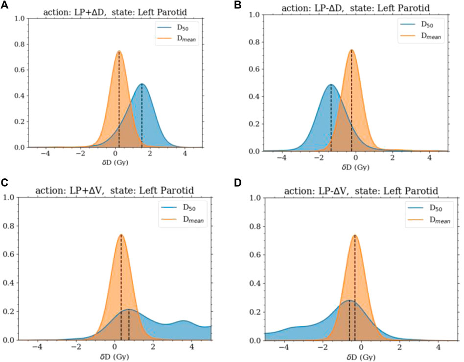
FIGURE 1. Distributions of the change in
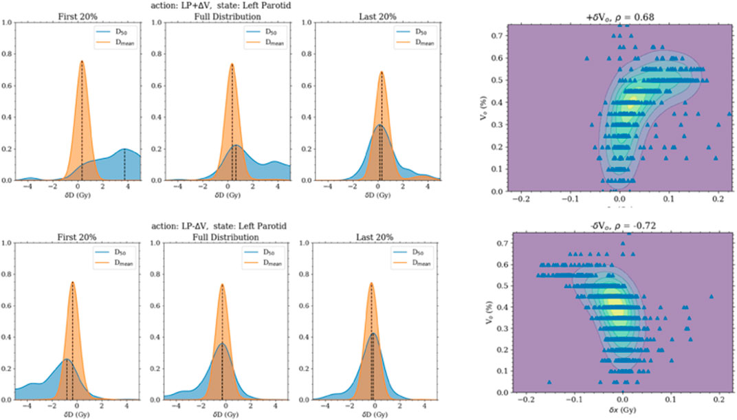
FIGURE 2. The left panels are the distribution of the change in the median and mean doses when the volume objective is changed. They are separated into the first 20%, last 20%, and all transitions. The first 20% transitions show a higher response in the change in median dose. The 2D plots of the right panel are of the change in the median dose with the initial volume objective.
Regarding checking the Markov property of the system, non-negligible correlations were found between the change in the state and past states when increasing or decreasing the volume objective. However, this was shown to be from the correlation of the current state and the past states. The current position of the volume objective was very highly correlated and, in some cases, completely determined by the past few states. No extra correlation was present between the transition and past states beyond the correlation between the states themselves.
3.2 Model analysis and validation
The first model (model 1) was successfully trained on the training set and tested on the testing set. In this model, the agent could only change the dose objective. Once trained, the agent was able to successfully plan for the given goals on the testing set. For each organ at risk goal (left parotid, right parotid, and oral cavity), the agent successfully acted to lower the median dose of each in an efficient manner. All of this was accomplished while maintaining PTV coverage. The agent was also observed to switch back and forth between OARs during planning. This is shown in Figure 3 as the agent planned for each goal simultaneously balancing against the need to cover the PTV. This contrasts with the planning done by purely selecting random actions where no goal was met. Figure 3 also shows that for the vast majority of plans, the agent was able to fully reduce the individual costs for the median doses connected to the OARs, while the random actions were not capable of accomplishing this. Thus, the agent learned to plan accordingly to the given actions. An inherent bias was observed in model 1 when trained only using a 15-case set. This was seen by the agent preferring to spare the left parotid over the right parotid. The bias can be seen in the differing weighting matrices. The state–action pair for lowering the left parotid objective and the current dose of the left parotid was much higher than that for lowering the right parotid objective and the current dose of the right parotid. This is shown in Figure 4 along with the magnitude of the corresponding state element–action pairs throughout training between the small and large training sets. The decision boundary slope between the state–action pairs of lowering the dose and the current dose of the parotids can be projected onto the dimensions of the state representing the dose of the left and right parotids. The slope of this projection would describe the bias between the two and is plotted in Figure 4 as well.
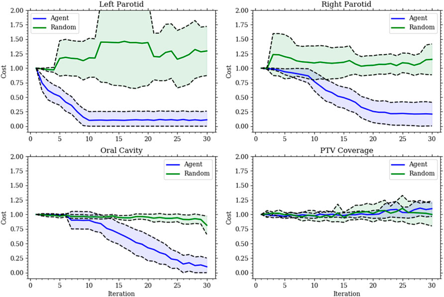
FIGURE 3. Each plot gives the relative cost, with an initial cost of 1, at each action step for model 1’s validation set. The solid lines are the mean, and the shaded region is the standard deviation for all validation sets. The (blue) agent consistently reduces the cost for all organs at risk while maintaining the target coverage. The (green) random agent is given to show the improbability of making the correct choices made by the agent.
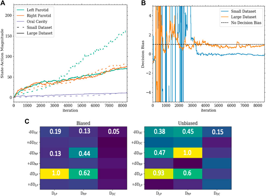
FIGURE 4. (A) This is a plot of the magnitudes of the state–action pairs in the weighting matrix throughout training. Each value corresponds to the magnitude of the pair corresponding to the action of lowering the dose for an organ and the state of the dose of that organ. (B) This is a plot of the slope of the decision boundary of the hyperplane between lowering the left parotid and the right parotid projected onto the portion of the state with the dose of the left and right parotids. In this configuration, a slope of 1 would indicate a completely unbiased decision boundary. (C) The bottom is a portion of the weighting matrices of the Q-function for the small dataset (biased) and large dataset (unbiased). The corresponding values highlight the asymmetry and symmetry between sparing the left and right parotids as well as the secondary importance of the oral cavity determined by the agent.
Interestingly, the agent learned to spare the oral cavity only secondarily to both parotids, even though equal weighting was given in the reward function. This can be seen in the decision boundaries. The region in which sparing of the oral cavity is preferred is much smaller than that for the parotids. The region’s size is dependent on the current dose of the oral cavity and grows linearly with it. The decision boundaries between the three organs are shown in Figure 5. The fact that the agent learned to spare the oral cavity secondary to the parotids is most likely due to the relative difficulty of reaching the goals between the organs. The oral cavity’s goal is normally much easier to reach than with the parotids. Thus, although the weighting in the reward function is the same, the parotids experience much higher rewards early on as they lie further away from the goal.
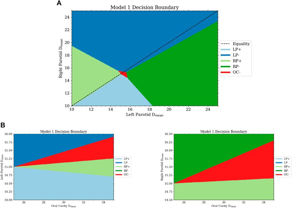
FIGURE 5. (A) This is a projection of the decision surface onto the right and left parotid mean dose portions of the state. It can be seen that there is little bias between the two from the slope of the boundary between lowering the objective on the left and right parotid. If the dose of the parotids is below some limit, then from the Q-function, the agent will want to increase the dose. With the dose of both parotids close to the goal, the space for lowering the oral cavity objective is activated. (B) The bottom two plots are projections of the decision surface onto the oral cavity mean dose and the left (bottom left) and right (bottom right) parotid mean doses.
Model 2 was also successfully trained and implemented. Analysis of the resulting weighting matrix showed a strategy in which there is a trading off between lowering the objective volume and dose for the parotid glands. This trade-off is a function of the current position of the objectives and the current mean dose. The weighting matrix and the section of the decision boundary for model 2 are shown in Figure 6. The observed strategy learned from the agent was to lower the dose of the parotids by a trade-off between lowering the objective volume and dose given the decision boundaries between the two. What was observed for the oral cavity was not only reducing its dose of secondary importance but that it was primarily achieved by lowering the dose objective only. When comparing the validated plans to plans produced simply by placing the template objectives, model 2 outperformed the template plans for both parotids, with an average reduction in the mean dose of 7 Gy
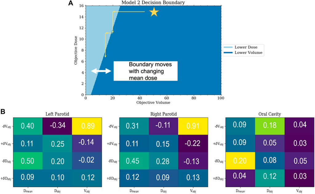
FIGURE 6. (A) This is a plot of the decision boundary between either lowering the objective volume or dose as a function of the current objective volume and dose. Initially, the agent will lower the volume until reaching the trade-off boundary and then begin lowering the dose until it hits the boundary again. This boundary is dynamic and moves to the right with the increasing mean dose. (B) Sections of the weighting matrix important to the parotids and oral cavity are zoomed in. The symmetry between the parotids can be seen. Not only can the reduced significance of the oral cavity be observed but also that the preference is to lower the objective dose and not the objective volume.
Model 2 produced plans with distributions that are highly comparable with those of the clinical plans. For comparisons with clinical plans, all plans were normalized such that PTV coverage was the same with
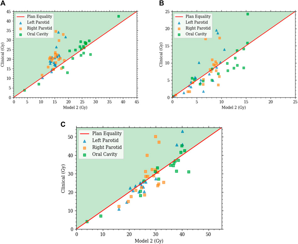
FIGURE 7. Each plot is a scatter plot for the dosimetric endpoints where each point is a specific plan between model 2 and the clinical plans for the (A) primary plan at 44 Gy, (B) boost plan at 26 Gy, and (C) plan sum.
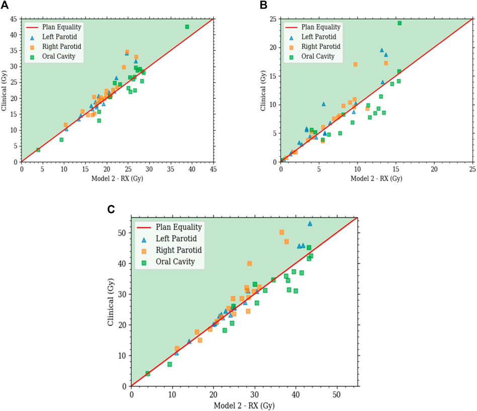
FIGURE 8. Each plot is a scatter plot for the dosimetric endpoints where each point is a specific plan between model 2 with state scaling and the clinical plans for the (A) primary plan at 44 Gy, (B) boost plan at 26 Gy, and (C) plan sum.
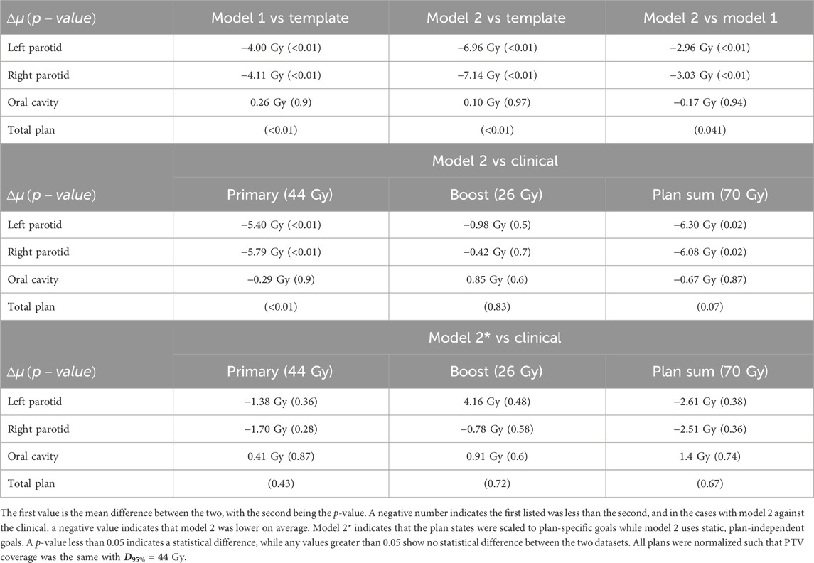
TABLE 1. Statistical analysis between models, template plans, and clinical plans.
With comparable dosimetry endpoints, model 2 produced slightly different DVH shapes compared to the clinical plans. The clinical plans had a sharper PTV DVH slope from a dose range of 95% to 105%, with fewer hotspots. The oral cavity DVH shapes were very similar between the two plans. For both parotids, even with similar final mean doses, the DVHs had noticeably different shapes in many cases. Typically, the clinical case DVHs were higher in the lower-dose regions and lower in the high-dose regions than those for model 2. Cross-over points often happened between 40% and 50% of the volume. For model 2, PTV coverage had comparable dose decreases to clinical plans, in the range from 90% to 50% dose. Model 2 produced less sparing of organs not included in the model like the spinal cord, larynx, and pharynx. These were included in optimization but with static plan-independent objectives. These static objectives may or may not reflect the optimal sparing of these organs and thus would lead to the observed discrepancies. Model 2 also had stronger normal tissue sparing as these were also not manipulated by the agent. A human planner may make the decision to sacrifice some normal tissue sparing, but the agent currently cannot make that decision. Some examples of the dose distribution are shown in Figure 9 and examples of the DVHs in Figure 10.
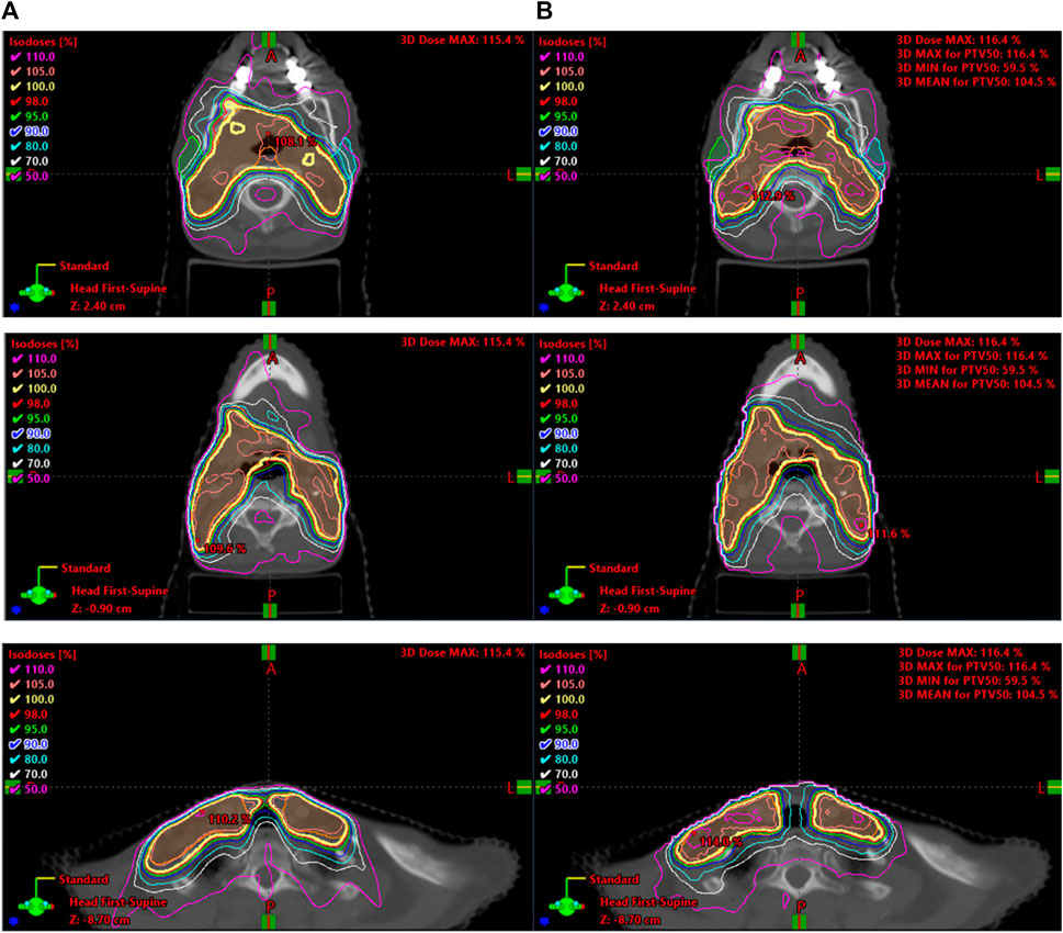
FIGURE 9. (A) Clinical vs. (B) agent-delivered dose distributions.
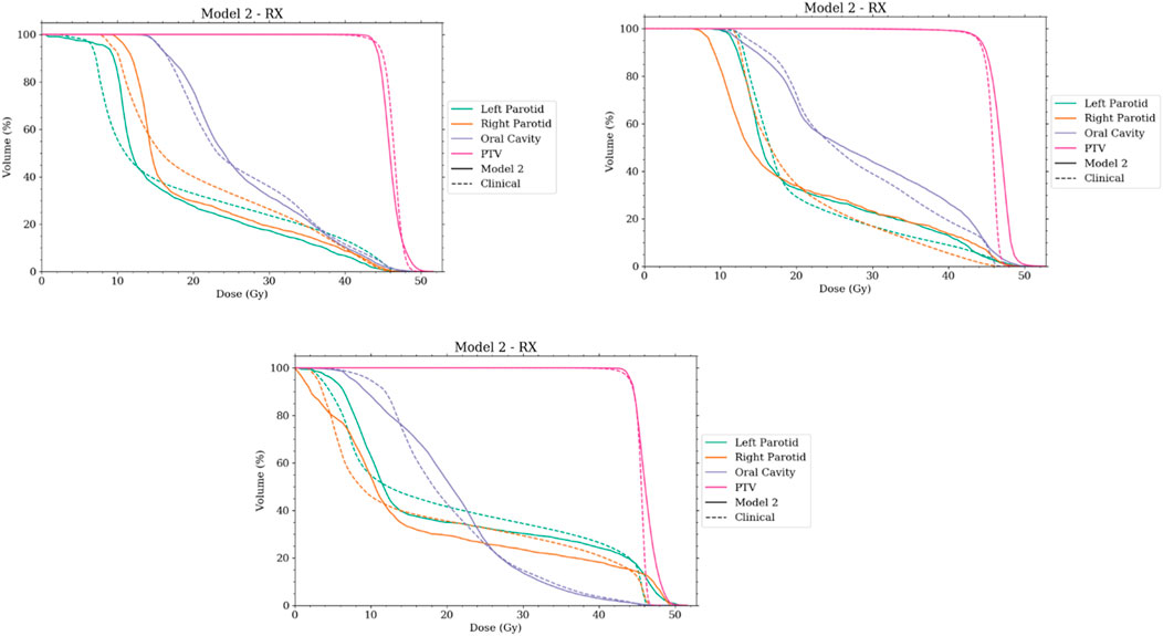
FIGURE 10. Selection of DVHs comparing the plans produced by model 2 to corresponding clinical plans. The solid lines represent the plans created by the auto-planning agent, while the dashed line represents the corresponding clinical plan. RX notes that the agent was using plan-specific goals.
4 Discussion
Overall, both models 1 and 2 showed significant steps toward the goal of producing an overall auto-planning agent. The models presented satisfy all conditions necessary in an MDP and provided a meaningful environment for agent learning. This is an important component to consider when developing an RL agent. Most of the models can take weeks to train, and increasing the size of the model will exponentially increase that time. Knowing the consistency of the environment is crucial with a lag time this large in between results.
It is not surprising that model 1 failed to plan for the mean dose after successfully planning for the median dose. The median dose is directly linked to a specific dose–volume objective, namely, the dose at 50% volume. So the response of this goal will be large when changing the specific objective as had been seen with the transition probabilities. What was also seen with the transition probabilities is that the mean dose had a much smaller response and thus would need more movement to completely reduce it to the desired amount. Thus, the movement in the volume space expanded the desired total movement amount. Hence, allowing the agent to move in the dose and volume space greatly improved the agent’s planning ability. Moving the objective diagonally in the dose–volume space will reduce the area under the curve more effectively than simply moving it in the dose space. It was also apparent from the strong correlation of the transition probabilities to the current location of the objective that including this information into the state function is crucial to provide the agent with as much needed information as possible.
Model 2 showed very promising results when compared to the clinical plans. In both scenarios of including and not including plan-specific goals, the agent produced statistically similar plans to that of those used in the clinic. This included producing very comparable and acceptable dose distributions. This is quite promising as the agent created these plans in a matter of minutes without human intervention. It should be noted though that only the three organs mentioned were included. For a fully automated planning agent, all organs would need to be considered and more objective control points may need to be added to the PTV to better control the coverage/hotspot trade-off. This can be built upon the framework presented.
Another interesting result was that of discovering the model bias that seemed to be dependent on the training set size. No apparent bias was found in the smaller training set when anatomical and geometric values were investigated. However, the small bias inherent to the set was exacerbated when using a small training set. This resulted in a slightly different final dosimetry as the biased organs had greater sparing. This may not be important for some cases, but if the agent is not able to get the preferred organ below a certain point, it could spend the entire planning time on it without considering the others. Currently, the agent has no way of giving up on a goal, and this could be an interesting avenue for future work.
Another limitation is the lack of heterogeneity correction in the dose calculation and optimization model. This is not a big difference for the sites studied here but could potentially pose issues when dealing with lung cases. The large air or vapor areas in the lungs can drastically affect photon and electron transport as compared to normal tissue or even bone. Thus, in these instances, larger differences due to heterogeneities could be present.
Computational cost is also a potential limitation to this and future studies. Model 1 exceeded 10,000 training iterations with only one objective per the three OARs, and model 2 reached over 24,000 training iterations. Therefore, using the current computation setup, it would be difficult to include multiple control points for multiple organs as well as more PTV objectives to ensure a sharp DVH for the target. Since the RL problem is iterative and is based on Markov decision chains, large-scale parallelization is not an option. The needed speed-up would need to be in the optimization step. With so many optimization steps, a small reduction in cost would potentially lead to a very large reduction for the entire training process.
Even given the methods mentioned in the introduction that can predict the achievable DVH or dosimetric endpoints for an OAR given the patient anatomy, it would be more complete to remove the goal as input and have it inferred by the agent. This would allow more flexibility and remove a prior step. To accomplish this goal, anatomical features would need to be included into the state function. It has already been shown that certain features are good predictors for the final achievable median dose [9]. These include the median distance from target, the overlap percentage between the organ and the target, and the total volume within an organ specific range. These would be simple factors to add into the state function to allow the agent spatial and anatomical information to adjudicate the goal for each of the glands.
There are few other limitations to this study that further work can improve on. The first is that a larger dataset from multiple institutions could be used. The reason for this is to incorporate a larger and more diverse patient population and include institutional differences in both the training and evaluation of the model. Another is a study on the selection of hyper-parameters. The long training time for the models limits the ability to tune hyper-parameters, and thus more work is needed in selecting these. Finally, this study also incorporates a discretized action space, when in reality a human planner can change the objectives by any real value and has control over all regions of interest. The addition of regions of interest must be done carefully in order to reduce the computational cost.
The SARSA algorithm presented is very simple. However, it has been shown to be powerful. The presented model architecture provides a very solid foundation with the ability to interpret the learning of the agent. These methods rely on relatively small datasets and provide the potential of moving into more deep learning methodologies as with increase in understanding.
5 Conclusion
An RL model was developed and tested for the purposes of creating IMRT plans for HN cancer treatment. The proposed models were based on including dosimetric and objective information in the state function and were shown to perform in a Markovian fashion that well-approximates the conditions required by an RL model. The proposed model was shown to make significant improvements over template plans, creating plans that were statistically similar to clinical plans and made in a fraction of the time. The methods and results presented here have shown that RL can be used to develop efficient IMRT planning agents that automatically create clinically acceptable plans in a matter of minutes. This will allow not only for building upon this model for HN cancers but for other treatment sites as well.
Data availability statement
The raw data supporting the conclusion of this article will be made available by the authors, without undue reservation.
Author contributions
HS: conceptualization, data curation, formal analysis, investigation, methodology, software, validation, visualization, and writing–original draft. XL: data curation, software, and writing–review and editing. YS: supervision and writing–review and editing. QW: conceptualization, methodology, project administration, resources, supervision, and writing–review and editing. YG: conceptualization, supervision, and writing–review and editing. QJW: conceptualization, funding acquisition, methodology, project administration, resources, supervision, and writing–review and editing.
Funding
The authors declare that financial support was received for the research, authorship, and/or publication of this article. This work was supported by an NIH Grant (#R01CA201212) as well as a Varian research grant.
Conflict of interest
The authors declare that the research was conducted in the absence of any commercial or financial relationships that could be construed as a potential conflict of interest.
The authors declared that they were an editorial board member of Frontiers, at the time of submission. This had no impact on the peer review process and the final decision.
Publisher’s note
All claims expressed in this article are solely those of the authors and do not necessarily represent those of their affiliated organizations, or those of the publisher, the editors, and the reviewers. Any product that may be evaluated in this article, or claim that may be made by its manufacturer, is not guaranteed or endorsed by the publisher.
References
1. Dawes C, Wood CM. The contribution of oral minor mucous gland secretions to the volume of whole saliva in man. Arch Oral Biol (1973) 18(3):337–42. doi:10.1016/0003-9969(73)90156-8
2. Deasy JO, Moiseenko V, Marks L, Chao KSC, Nam J, Eisbruch A. Radiotherapy dose–volume effects on salivary gland function. Int J Radiat Oncol Biol Phys (2010) 76(3):S58–63. doi:10.1016/j.ijrobp.2009.06.090
3. Patrik Brodin N, Tomé WA. Revisiting the dose constraints for head and neck OARs in the current era of IMRT. Oral Oncol (2018) 86:8–18. doi:10.1016/j.oraloncology.2018.08.018
4. Wang ZH, Zhang SZ, Zhang ZY, Zhang CP, Hu HS, Tu WY, et al. Protecting the oral mucosa in patients with oral tongue squamous cell carcinoma treated postoperatively with intensity-modulated radiotherapy: a randomized study. The Laryngoscope (2012) 122(2):291–8. doi:10.1002/lary.22434
5. Lee N, Puri DR, Blanco AI, Chao KSC. Intensity-modulated radiation therapy in head and neck cancers: an update. Head Neck (2007) 29(4):387–400. doi:10.1002/hed.20332
6. Gupta T, Agarwal J, Jain S, Phurailatpam R, Kannan S, Ghosh-Laskar S, et al. Three-dimensional conformal radiotherapy (3D-CRT) versus intensity modulated radiation therapy (IMRT) in squamous cell carcinoma of the head and neck: a randomized controlled trial. Radiother Oncol J Eur Soc Ther Radiol Oncol (2012) 104(3):343–8. doi:10.1016/j.radonc.2012.07.001
7. Hunt MA, Jackson A, Narayana A, Lee N. Geometric factors influencing dosimetric sparing of the parotid glands using IMRT. Int J Radiat Oncol Biol Phys (2006) 66(1):296–304. doi:10.1016/j.ijrobp.2006.05.028
8. Anand AK, Jain J, Negi PS, Chaudhoory AR, Sinha SN, Choudhury PS, et al. Can dose reduction to one parotid gland prevent xerostomia? A feasibility study for locally advanced head and neck cancer patients treated with intensity-modulated radiotherapy. Clin Oncol R Coll Radiol G B (2006) 18(6):497–504. doi:10.1016/j.clon.2006.04.014
9. Yuan L, Ge Y, Lee WR, Yin FF, Kirkpatrick JP, Wu QJ. Quantitative analysis of the factors which affect the interpatient organ-at-risk dose sparing variation in IMRT plans. Med Phys (2012) 39(11):6868–78. doi:10.1118/1.4757927
10. Wu B, Ricchetti F, Sanguineti G, Kazhdan M, Simari P, Chuang M, et al. Patient geometry-driven information retrieval for IMRT treatment plan quality control. Med Phys (2009) 36(12):5497–505. doi:10.1118/1.3253464
11. Moore KL, Brame RS, Low DA, Mutic S. Experience-based quality control of clinical intensity-modulated radiotherapy planning. Int J Radiat Oncol Biol Phys (2011) 81(2):545–51. doi:10.1016/j.ijrobp.2010.11.030
12. Zhu X, Ge Y, Li T, Thongphiew D, Yin FF, Wu QJ. A planning quality evaluation tool for prostate adaptive IMRT based on machine learning. Med Phys (2011) 38(2):719–26. doi:10.1118/1.3539749
13. Appenzoller LM, Michalski JM, Thorstad WL, Mutic S, Moore KL. Predicting dose-volume histograms for organs-at-risk in IMRT planning. Med Phys (2012) 39(12):7446–61. doi:10.1118/1.4761864
14. Yuan L, Wu QJ, Yin FF, Jiang Y, Yoo D, Ge Y. Incorporating single-side sparing in models for predicting parotid dose sparing in head and neck IMRT. Med Phys (2014) 41(2):021728. doi:10.1118/1.4862075
15. Kuo YH, Liang JA, Wang TC, Juan CJ, Li CC, Chien CR. Comparative effectiveness of simultaneous integrated boost vs sequential intensity-modulated radiotherapy for oropharyngeal or hypopharyngeal cancer patients. Medicine (Baltimore) (2019) 98(51):e18474. doi:10.1097/md.0000000000018474
16. Nelms BE, Robinson G, Markham J, Velasco K, Boyd S, Narayan S, et al. Variation in external beam treatment plan quality: an inter-institutional study of planners and planning systems. Pract Radiat Oncol (2012) 2(4):296–305. doi:10.1016/j.prro.2011.11.012
17. Sheng Y, Zhang J, Ge Y, Li X, Wang W, Stephens H, et al. Artificial intelligence applications in intensity modulated radiation treatment planning: an overview. Quant Imaging Med Surg (2021) 11(12):4859–80. doi:10.21037/qims-21-208
18. Kubo K, Monzen H, Ishii K, Tamura M, Kawamorita R, Sumida I, et al. Dosimetric comparison of RapidPlan and manually optimized plans in volumetric modulated arc therapy for prostate cancer. Phys Med PM Int J Devoted Appl Phys Med Biol Off J Ital Assoc Biomed Phys AIFB (2017) 44:199–204. doi:10.1016/j.ejmp.2017.06.026
19. Li N, Carmona R, Sirak I, Kasaova L, Followill D, Michalski J, et al. Highly efficient training, refinement, and validation of a knowledge-based planning quality-control system for radiation therapy clinical trials. Int J Radiat Oncol Biol Phys (2017) 97(1):164–72. doi:10.1016/j.ijrobp.2016.10.005
20. Scaggion A, Fusella M, Roggio A, Bacco S, Pivato N, Rossato MA, et al. Reducing inter- and intra-planner variability in radiotherapy plan output with a commercial knowledge-based planning solution. Phys Med PM Int J Devoted Appl Phys Med Biol Off J Ital Assoc Biomed Phys AIFB (2018) 53:86–93. doi:10.1016/j.ejmp.2018.08.016
21. Hussein M, South CP, Barry MA, Adams EJ, Jordan TJ, Stewart AJ, et al. Clinical validation and benchmarking of knowledge-based IMRT and VMAT treatment planning in pelvic anatomy. Radiother Oncol J Eur Soc Ther Radiol Oncol (2016) 120(3):473–9. doi:10.1016/j.radonc.2016.06.022
22. Tol JP, Delaney AR, Dahele M, Slotman BJ, Verbakel WFAR. Evaluation of a knowledge-based planning solution for head and neck cancer. Int J Radiat Oncol Biol Phys (2015) 91(3):612–20. doi:10.1016/j.ijrobp.2014.11.014
23. Chang ATY, Hung AWM, Cheung FWK, Lee MCH, Chan OSH, Philips H, et al. Comparison of planning quality and efficiency between conventional and knowledge-based algorithms in nasopharyngeal cancer patients using intensity modulated radiation therapy. Int J Radiat Oncol Biol Phys (2016) 95(3):981–90. doi:10.1016/j.ijrobp.2016.02.017
24. Shen C, Nguyen D, Chen L, Gonzalez Y, McBeth R, Qin N, et al. Operating a treatment planning system using a deep-reinforcement learning-based virtual treatment planner for prostate cancer intensity-modulated radiation therapy treatment planning. Med Phys (2020) 47(6):2329–36. doi:10.1002/mp.14114
25. Sprouts D, Gao Y, Wang C, Jia X, Shen C, Chi Y. The development of a deep reinforcement learning network for dose-volume-constrained treatment planning in prostate cancer intensity modulated radiotherapy. Biomed Phys Eng Express (2022) 8(4):045008. doi:10.1088/2057-1976/ac6d82
26. Gao Y, Shen C, Jia X, Kyun Park Y. Implementation and evaluation of an intelligent automatic treatment planning robot for prostate cancer stereotactic body radiation therapy. Radiother Oncol (2023) 184:109685. doi:10.1016/j.radonc.2023.109685
27. Wang H, Bai X, Wang Y, Lu Y, Wang B. An integrated solution of deep reinforcement learning for automatic IMRT treatment planning in non-small-cell lung cancer. Front Oncol (2023) 13:1124458. doi:10.3389/fonc.2023.1124458
28. Zhang J, Wang C, Sheng Y, Palta M, Czito B, Willett C, et al. An interpretable planning bot for pancreas stereotactic body radiation therapy. Int J Radiat Oncol (2021) 109(4):1076–85. doi:10.1016/j.ijrobp.2020.10.019
29. Stephens H, Wu QJ, Wu Q. Introducing matrix sparsity with kernel truncation into dose calculations for fluence optimization. Biomed Phys Eng Express (2021) 8(1):8. doi:10.1088/2057-1976/ac35f8
30. Sutton RS, Barto AG. Reinforcement learning: an introduction. In: F Bach, editor. Adaptive computation and machine learning series. Cambridge, MA, USA: A Bradford Book (1998). p. 344.
Keywords: reinforcement learning, radiation therapy, automated treatment planning, head and neck cancer, interpretable machine learning
Citation: Stephens H, Li X, Sheng Y, Wu Q, Ge Y and Wu QJ (2024) A reinforcement learning agent for head and neck intensity-modulated radiation therapy. Front. Phys. 12:1331849. doi: 10.3389/fphy.2024.1331849
Received: 01 November 2023; Accepted: 15 January 2024;
Published: 01 February 2024.
Edited by:
Xun Jia, Johns Hopkins Medicine, United StatesReviewed by:
Yin Gao, University of Texas Southwestern Medical Center, United StatesWilliam Hrinivich, Johns Hopkins University, United States
Copyright © 2024 Stephens, Li, Sheng, Wu, Ge and Wu. This is an open-access article distributed under the terms of the Creative Commons Attribution License (CC BY). The use, distribution or reproduction in other forums is permitted, provided the original author(s) and the copyright owner(s) are credited and that the original publication in this journal is cited, in accordance with accepted academic practice. No use, distribution or reproduction is permitted which does not comply with these terms.
*Correspondence: Q. Jackie Wu, amFja2llLnd1QGR1a2UuZWR1