Noise-induced synchronization and regularity in feed-forward-loop motifs

This study explores the impacts of multiple factors (noise, intra-motif coupling, and critical bifurcation parameter) on noise-induced motif synchrony and output regularity in three-node feed-forward-loops (FFLs), distinguishing between coherent FFLs with purely excitatory connections and incoherent FFLs formed by transitioning the intermediate layer to inhibitory connections. Our model utilizes the normal form of Hopf bifurcation (HB), which captures the generic structure of excitability observed in real systems. We find that the addition of noise can optimize motif synchrony and output regularity at the intermediate noise intensities. Our results also suggest that transitioning the excitatory coupling between the intermediate and output layers of the FFL to inhibitory coupling—i.e., moving from the coherent to the incoherent FFL—enhances output regularity but diminishes motif synchrony. This shift towards inhibitory connectivity highlights a trade-off between motif synchrony and output regularity and suggests that the structure of the intermediate layer plays a pivotal role in determining the motif’s overall dynamics. Surprisingly, we also discover that both motifs achieve their best output regularity at a moderate level of intra-motif coupling, challenging the common assumption that stronger coupling, especially of the excitatory type, results in improved regularity. Our study provides valuable insights into functional differences in network motifs and offers a direct perspective relevant to the field of complex systems as we consider a normal-form model that pertains to a vast number of individual models experiencing HB.

1 Introduction

Network motifs, a fundamental concept in network analysis, refer to recurring interaction patterns observed across diverse systems [1, 2]. Multiple systematic research studies have provided robust evidence for the widespread prevalence of these motifs within real biological networks, with a particular emphasis on complex networks [3–5]. As these motifs often retain their specific dynamical functions when embedded within complex network structures, they are often considered to be the basic building blocks or elementary computational units of larger, more complex networks [4, 6].

Among the common three-node network motifs, feed-forward-loops (FFLs) are notably more prevalent than other motif patterns [4, 5]. In this paper, we focus on two prevalent FFL motifs: the coherent FFL, characterized by purely excitatory connections, and the incoherent FFL, formed by two excitatory connections, and one inhibitory connection, as illustrated in Figure 1. We shall refer to them as type-1 (T1) and type-2 (T2), respectively. These two FFL motifs have been identified in a multitude of biological networks, including gene expression networks in bacteria and yeast [3, 7, 8], human and mouse genomes [9, 10], the cat cortex [11], and the nervous system of the roundworm [3]. Moreover, these motifs can be considered as having three primary layers: an input layer (node 1), an intermediate layer (node 2), and an output layer (node 3). These motifs incorporate two parallel signalling pathways between the input and output layers: a direct pathway from the input layer to the output layer, and an indirect pathway from input to output via the intermediate layer. Notably, such parallel information transmission structures have been observed in the auditory cortex [12], the electrosensory system [13], and more generally, regions responsible for transmitting signals from sensory neurons to effectors [3, 14].

FIGURE 1

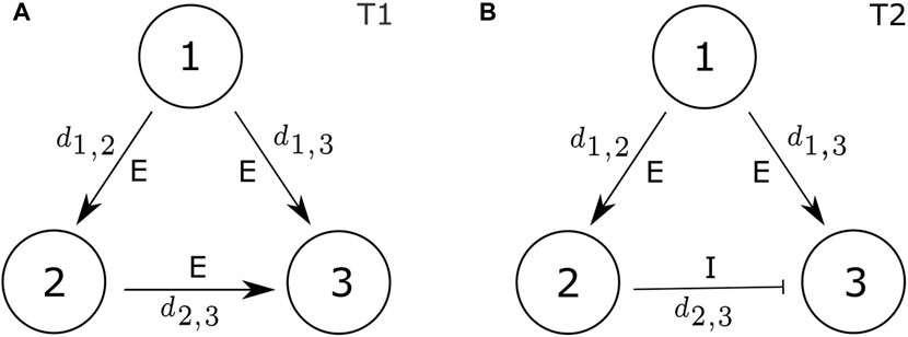
FIGURE 1. Coherent and incoherent feed-forward-loop motifs: (A) motif type 1 (T1); and (B) motif type 2 (T2). d_i,j represents the coupling strength within the motif, specifically indicating the strength of the connection from node i to node j. “E” denotes excitatory coupling (d_i,j > 0) and “I” denotes inhibitory coupling (d_i,j < 0).

Phase synchrony, commonly observed in network dynamics, denotes the synchronized timing of oscillatory activity across network components. It has diverse applications, for examples, it mirrors neural coordination and cognitive functions in neuroscience [15, 16], it unveils collective behaviours and synchronization transitions in physics [17, 18], and it assists in optimizing communication systems for effective signal transmission in engineering [19, 20]. Within network motifs, synchrony illustrates how particular connectivity patterns influence coordination and coherence, aiding in revealing the mechanisms driving collective network behaviours, information processing, and functional dynamics in various biological and engineered systems. Noise, intrinsic to many natural and engineered systems, introduces fluctuations that can either enhance or disrupt synchrony among network elements [21, 22]. Understanding how noise influences synchrony within network motifs is crucial for discovering the robustness and adaptability of network structures to environmental perturbations, thus offering valuable insights into the resilience and functionality of complex networks. Several investigations have explored the dynamics of FFLs under conditions involving symmetric noise (where each node experiences independent noise sources with identical intensities) and equal coupling (e.g., equivalent coupling strength) [23–25]. However, prior studies have not addressed the behaviours of FFL motifs under more realistic configurations, such as unequal coupling and asymmetric noise. Hence, this paper explores their dynamics considering two forms of heterogeneity: independent noise sources with varying intensities and distinct coupling strengths.

To capture the excitability characteristic of real systems, we employ the widely recognized framework of the Hopf bifurcation (HB). This framework describes the system’s transition from a stable equilibrium state to persistent oscillations, a phenomenon frequently observed in real complex systems. Specifically, we utilize the standard λ − ω system, a canonical model of the Hopf bifurcation, to simulate the dynamics of individual nodes within the FFL motifs. We focus on the excitable regime, where the deterministic system maintains a stable equilibrium, but the introduction of noise can induce oscillations. Our study demonstrates that the addition of noise can optimize network motif synchrony and oscillation regularity of the output node at an intermediate intensity level. Furthermore, we reveal substantial differences in how each motif type responds to noise-induced excitation, shedding light on the functional distinctions between these network motifs.

This paper is structured as follows: Section 2 presents the mathematical model and methods. In Section 3.1, we explore the noise-induced dynamics of two FFL motifs. Section 3.2 investigates the effects of noise on motif synchronization; while Section 3.3 delves into the influence of noise on output regularity. Section 3.4 is dedicated to the study of the combined effects of noise and intra-motif coupling on motif synchrony and output regularity. In Section 3.5, we examine how the control parameter of HB impacts motif synchronization and output regularity. Finally, the paper concludes with a discussion in Section 4.

2 Materials and methods

2.1 Model

We consider a system comprised of three coupled nodes arranged in FFL patterns (see Figure 1), where the dynamics of each node are described by the canonical model for the normal form of an HB, the λ − ω system, with additive noise and diffusive coupling terms. The i-th node is modeled by the system of stochastic differential equations (SDEs).

$d{x}_i=[\lambda \left(r_i\right)x_i-\omega \left(r_i\right)y_i+{\displaystyle \sum _{j\ne i}}{d}_{j,i}\left(x_j-x_i\right)]dt+{\delta }_{i}d{\eta }_i\left(t\right),(1)$

$d{y}_i=[\omega \left(r_i\right)x_i+\lambda \left(r_i\right)y_i+{\displaystyle \sum _{j\ne i}}{d}_{j,i}\left(y_j-y_i\right)]dt,(2)$

where i, j = 1, 2, 3.

The amplitude and phase of the i-th node can be determined by the equations $r_i=\sqrt{x_i^2+y_i^2}$ and ϕ_i = arctan(y_i/x_i), respectively. The function $\lambda (r_i)={\lambda }_0+\alpha r_i^2+\rho r_i^4$ governs the modulation of the amplitude of the i-th node. λ₀ acts as the critical bifurcation parameter, commonly known as the control parameter, while α and γ govern the behaviours of the nodes within the excitable regime. Specifically, under conditions where α < 0 and ρ < 0, each node operates within a framework of supercritical HB when λ₀ = 0. The function $\omega (r_i)={\omega }_0+{\omega }_1{r}_i^2$ controls the modulation of the frequency of the i-th node, with ω₁ governing how the frequency evolves in relation to the amplitude r_i. Notably, when ω₁ = 0, changes in amplitude do not directly impact the phase. As a continuation of our previous work on the noise-induced dynamics in single oscillators (i.e., one-node motif) [26] and two-node motifs [27], we maintain the same parameter values: α = −0.2, ρ = −0.2, ω₀ = 2, and ω₁ = 0. The term δ_idη_i(t) represents an intrinsic white noise applied to x_i, where η_i(t), i = 1, 2, 3 are three independent Wiener processes with zero mean and unit variance, i.e., η₁(t) ≠ η₂(t) ≠ η₃(t), and δ_i is a scaling parameter which represents the noise intensity.

The expressions ∑_j≠id_j,i(x_j − x_i) and ∑_j≠id_j,i(y_j − y_i) represent the contributions of diffusive coupling to each node. d_j,i represents a scalar parameter indicating the strength of a signal transmitted from node j to node i. Importantly, d_j,i ≠ d_i,j due to the directional nature of the motif graph. To construct the feed-forward-loop (FFL) motifs depicted in Figure 1, we set d_j,1 = 0 and d_3,i = 0 for all i and j. This configuration ensures that node 1 remains isolated from external input within the FFL, while node 3 does not convey its output to other nodes within the same FFL. Moreover, in motif T1, all three connections are excitatory, that is, d_1,2 > 0, d_1,3 > 0, and d_2,3 > 0, and in motif T2, there are two excitatory connections (d_1,2 > 0 and d_1,3 > 0), complemented by a single inhibitory connection (d_2,3 < 0).

2.2 Methods

All computational tasks, including simulation, numerical analysis, and figure generation, are conducted using MATLAB. The numerical solutions to the SDEs are computed using the Euler-Maruyama method and a time step of dt = 0.01. We initiate the simulations with arbitrary, small random initial conditions x_i(0), y_i(0), i = 1, 2, 3, each drawn from the distribution N(0, 0.008²). To address the challenges posed by the high-frequency fluctuations inherent in noise-induced dynamics, we implement a low-pass filter during the numerical analysis. This filter takes the form of a Gaussian-weighted moving average, spanning a window of 100 data points. Finally, the computation of coherence measures σ, γ, and CV, as defined in Eqs 4–6, involves averaging these values across a total of N = 200 simulations. The MATLAB source code can be found at https://github.com/TMUcode/FFL-synchrony.

3 Results

3.1 Noise-induced dynamics

We explore the dynamics of the network motifs within the excitable regime, λ₀ < 0, and in close proximity to a supercritical HB at λ₀ = 0 (e.g., λ₀ = −0.3 as illustrated in Figure 2). The deterministic systems (δ_i = 0 for i = 1, 2, 3) associated with motifs T1 and T2 converge towards a stable fixed point located at the origin (0,0), as shown in Figures 2A, D, respectively. We observe that all three nodes in motif T1 achieve in-phase oscillations in spite of their differing initial values (Figure 2A). Conversely, in the case of deterministic motif T2, nodes 1 and 2 exhibit in-phase oscillations, whereas node 3 displays anti-phase oscillations with nodes 1 and 2 (Figure 2D) due to the inhibitory connection. In both motifs, nodes 1 and 2 demonstrate identical behaviors since their differences lie solely in their connection types to output node (node 3). However, the introduction of independent noise prompts them to display distinct dynamics.

FIGURE 2

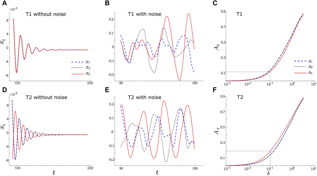
FIGURE 2. (A,D): Example timeseries of x_i without noise (setting noise intensities to zero, δ_i = 0, i = 1, 2, 3) for motifs T1 and T2, respectively. In the absence of noise, all three nodes evolve into the stable solutions with x_i = 0. (B,E): Example noise-induced oscillations of x_i (δ_i = 0.1, i = 1, 2, 3) for motifs T1 and T2, respectively. Each node receives independent noise stimuli, therefore distinct oscillations are induced in each node. (C,F): The average amplitude, A_i (see Eq. 3) vs. noise intensity, δ, for motifs T1 and T2, respectively. Here we consider a simple case with equal noise intensities for all nodes (δ₁ = δ₂ = δ₃ = δ), but they differ in other figures. In panels A, B, D and E, dashed blue, dotted black, and solid red lines represent x₁, x₂, and x₃, respectively. In panels C and F, dashed blue, dotted black, and solid red lines represent A₁, A₂, and A₃, respectively, while the grey dashed lines indicate the values of A₃ when δ = 0.1. Other parameters are: α = −0.2; ρ = −0.2; ω₀ = 2; ω₁ = 0; λ₀ = −0.3; d_1,3 = d_2,3 = d_1,2 = 0.01 for T1; and d_1,3 = −d_2,3 = d_1,2 = 0.01 for T2.

The introduction of the independent intrinsic noise stimulus, δ_idη_i(t) for i = 1, 2, 3, gives rise to sustained limit-cycle oscillations in all nodes within the T1 and T2 motifs, as observed in Figures 2B, E, where δ_i = 0.01 for i = 1, 2, 3. This type of oscillation is commonly referred to as “noise-induced oscillation.” Upon examining the noise-induced oscillations of the input nodes (i.e., node 1) in both the T1 and T2 motifs (blue dashed lines in Figures 2B, E), we note similarities in their periods and time-varying amplitudes. Similar observations arise when comparing nodes 2 in motifs T1 and T2 (dotted black lines in Figures 2B, E). However, a notable distinction emerges as we shift our focus to the output nodes (nodes 3) within the T1 and T2 motifs. The output node of the T2 motif (red curve in Figure 2E) displays more regular and stable oscillations, characterized by more prominent peaks and fewer small amplitude fluctuations, as compared to the output node in the T1 motif (red curve in Figure 2B).

To determine whether similar trends hold for various other noise intensities, we compute the time-averaged amplitude of x_i as

$A_i=\frac{1}{T-t_0}{\int }_{t_0}^T|x_i\left(t\right)|dt,i=\mathrm{1,2,3},(3)$

where T and t₀ denote the final and initial time points, respectively. We compute this metric over varying noise intensities and average over N = 200 trials. Our findings are depicted in Figure 2C for motif T1 and Figure 2F for motif T2. For simplicity, we assume equal noise intensity here, i.e., δ = δ₁ = δ₂ = δ₃, although they are distinct in subsequent analyses. The dashed blue lines represent A₁, the dotted black lines represent A₂, and the solid red lines represent A₃. We observe that A₁ and A₂ overlap for both T1 and T2 motifs, suggesting a strong resemblance in the behaviours of nodes 1 and 2 across various noise intensities. However, a noticeable discrepancy arises in the case of A₃ between motifs T1 and T2: A₃ in motif T2 surpasses its counterpart in motif T1. For instance, when δ₁, δ₂, δ₃ = 0.1, we observe that A₃ is approximately 0.12 for motif T1, while for motif T2, it reaches around 0.19 (as indicated by the dashed grey lines in Figures 2C, F). Moreover, the evaluation of the three A_i values within each motif reveals that in motif T1, A₃ is less than or equal to A₁ and A₂, while in motif T2, A₃ is greater than or equal to A₁ and A₂. These observations suggest that the inhibitory connection between the intermediate node and output node in motif T2 enhances the amplitude of noise-induced oscillations.

3.2 The effects of noise on motif synchronization

Here we keep the independent noise applied to the intermediate node and output node fixed at a relatively weak level (δ₂ = δ₃ = 0.01) and vary the noise intensity applied to the input node (e.g., δ₁ ∈ [10^–3, 10^1/2]). To investigate the influence of noise on the motif synchrony from different viewpoints, we adopt two measures to assess motif synchronization. The first measure quantifies the degree of motif synchronization among all nodes within each FFL motif using the root mean square deviation [28, 29]:

$\sigma =\frac{1}{T-t_0}{\int }_{t_0}^T{\sigma }_{t}dt,(4)$

where σ_t is defined as

${\sigma }_t=\sqrt{\frac{1}{M}{\displaystyle \sum _{i=1}^M}{\left(\frac{x_i\left(t\right)}{A_i}\right)}^2-{\left(\frac{1}{M}{\displaystyle \sum _{i=1}^M}\frac{x_i\left(t\right)}{A_i}\right)}^2},(5)$

and M represents the total number of nodes; here M = 3. It is important to note that σ_t is computed using the amplitude-normalized time series, x_i(t)/A_i, instead of using the raw x_i(t) data. This normalization ensures that σ serves as a metric for temporal synchronization, or phase synchronization, rather than a measure of complete synchronization, which involves both amplitude and phase alignment [30]. σ quantifies the extent of variability among three nodes, so smaller values of σ indicate higher levels of synchrony.

Figure 3A illustrates how motif synchrony changes with variations in noise intensity. It presents the relationship between the root mean square deviation, σ, and the driving noise intensity, δ₁, for both the T1 motif (blue curve) and the T2 motif (black curve). Both motifs display a resonant response to variations in δ₁, a phenomenon characteristic of coherence resonance. Coherence resonance or autonomous stochastic coherence describes the phenomenon where a nonlinear system achieves optimal coherence or synchronization in the presence of an optimal level of noise and this system remains inactive in the absence of noise [31, 32]. When δ₁ remains relatively low (e.g., δ₁ < 0.12 in Figure 3A), σ decreases for both motifs, indicating an increase in motif synchrony. At an intermediate noise intensity (e.g., δ₁ ≈ 0.12 in Figure 3A), σ reaches its minimum, indicating that motif synchronization reaches an optimal state. As the noise intensity continues to rise, σ begins to increase, signifying a decline in motif synchrony. This suggests that under the influence of relatively strong noise intensity, the noise itself has taken precedence in determining network dynamics, with the impact of motif structure on motif synchrony significantly reduced.

FIGURE 3

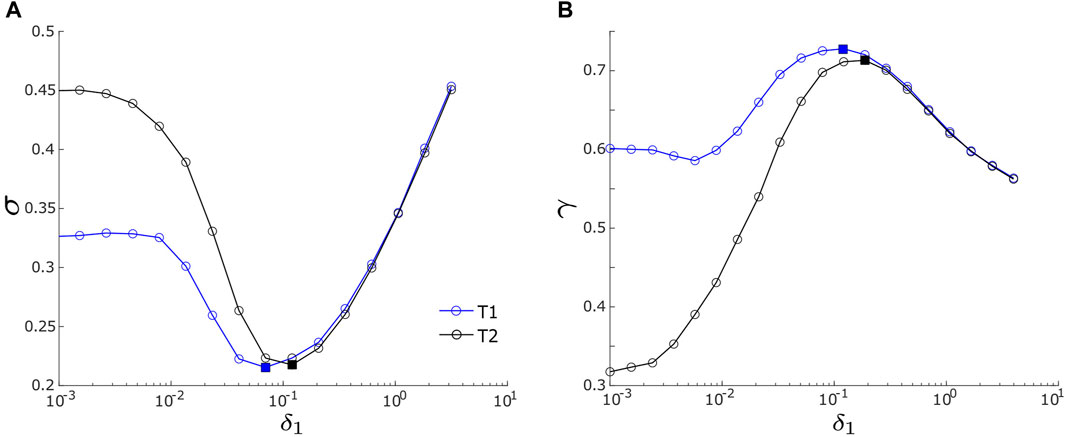
FIGURE 3. (A) Root mean square deviation, σ, vs. noise intensity, δ₁. (B) Mean phase coherence, γ, vs. noise intensity, δ₁. Two measures, σ and γ, are defined in Eqs 4 and 6, respectively. In both panels, blue and black lines represent the T1 motif and the T2 motif, respectively. The blue squares label the lowest σ in panel (A) or the highest γ in panel (B) for motif T1; the black squares label the lowest σ in panel (A) or the highest γ in panel (B) for motif T2. Motif T1 has d_2,3 = 0.1, and motif T2 has d_2,3 = −0.1. Other parameters are same for both motifs, including d_1,3 = d_1,2 = 0.1; α = −0.2; ρ = −0.2; ω₀ = 2; ω₁ = 0; δ₂ = δ₃ = 0.01; and λ₀ = −0.1.

While the synchrony generated by each motif exhibits a resonance pattern and they share similarities within the strong noise intensity range of δ₁, they exhibit notable differences in the weak and intermediate intensity ranges (e.g. δ₁ ≤ 0.1 in Figure 3A). In this regime, motif T1 consistently maintains σ values lesser than those of motif T2, indicating that T1 tends to exhibit greater motif synchrony. Additionally, the two motifs have differences concerning the optimal driving noise intensity denoted as ${\delta }_1^{*}$, and the absolute minimum value it induces, represented as σ*. Motif T1 demonstrates a lower σ* at a smaller ${\delta }_1^{*}$ in comparison to motif T2. As demonstrated by the solid squares in Figure 3A, ${\delta }_1^{*}=0.07$ and σ* = 0.215 for motif T1, and ${\delta }_1^{*}=0.12$ and σ* = 0.218 for motif T2. This indicates that the T1 motif can achieve a relatively greater degree of motif synchrony with a smaller driving noise intensity.

The second measure of motif synchrony focuses on evaluating the motif synchronization between the input and output nodes of the FFL motifs, specifically node 1 and node 3. To quantify this motif synchronization, we utilize the mean phase coherence [30, 33], denoted as γ.

$\gamma =\sqrt{{\left(\frac{1}{T-t_0}{\int }_{t_0}^T\sin \mathrm{\Delta }\varphi dt\right)}^2+{\left(\frac{1}{T-t_0}{\int }_{t_0}^T\cos \mathrm{\Delta }\varphi dt\right)}^2},(6)$

where Δϕ = |ϕ₁ − ϕ₃|, representing phase difference between node 1 and node 3. γ ranges from 0 to 1, with higher values representing a greater degree of phase synchronization between the input and output nodes. Moreover, γ = 1 corresponds to perfect synchronization, while γ = 0 indicates complete asynchrony.

The relationship between γ and the driving noise intensity, δ₁ is demonstrated in Figure 3B. Similar to σ in Figure 3A, γ in Figure 3B is computed over the range of 10^–3 ≤ δ₁ ≤ 10^1/2, with δ₂ and δ₃ held constant at 0.01. The results in Figure 3B agree with the findings from Figure 3A for both motifs. First, γ exhibits a resonance pattern: as δ₁ increases, γ initially ascends, reaches its peak, and then descends, indicating that phase synchronization between input and output nodes attains a maximum at an optimal noise intensity. Second, in comparison with the T2 motif, the T1 motif achieves a higher maximal γ value at a slightly lower optimal noise intensity. As illustrated in Figure 3B, the T1 motif reaches its maximum at ${\delta }_1^{*}=0.12$ with γ* = 0.728, while the T2 motif attains its maximum at ${\delta }_1^{*}=0.188$ with γ* = 0.713. Thirdly, when δ₁ exceeds 0.13, the γ values for both motifs become nearly identical, indicating that in the presence of relatively high noise intensity, the primary driver shaping noise-induced motif synchrony is the noise itself, rather than the motif structure.

3.3 The effects of noise on output regularity

In addition to our examination of the influence of noise on motif synchronization, we also investigate how it impacts the regularity of noise-induced oscillation of the output node (i.e., node 3) in both the T1 and T2 motifs. Here regularity refers to the extent to which the dynamics of the output node display perfect periodicity. It is measured by the coefficient of variation (CV) of the periods of x₃ as shown in Figure 4A inset. CV is defined as the ratio of the standard deviation of the periods to the mean of the periods [34–36],

$CV=\frac{\sqrt{\frac{1}{K-1}{\displaystyle {\sum }_{k=1}^{K-1}}{\left({\text{T}}_k\right)}^2-{\left(\frac{1}{K-1}{\displaystyle {\sum }_{k=1}^{K-1}}{\text{T}}_k\right)}^2}}{\frac{1}{K-1}{\displaystyle {\sum }_{k=1}^{K-1}}\left({\text{T}}_k\right)},(7)$

where T_k is the k-th period, where K − 1 denotes the total number of periods (signifying that there are K − 1 periods between K total peaks). To determine a period, we first detect spike events by identifying peaks in the time series of x₃, as depicted in the inset of Figure 4A. Subsequently, we compute the time difference between consecutive spike occurrences. Additionally, since the coefficient CV serves as a measure of central variability, it’s important to note that higher values of CV correspond to a less regular firing pattern and, therefore, reduced regularity, while lower values indicate a higher degree of regularity.

FIGURE 4

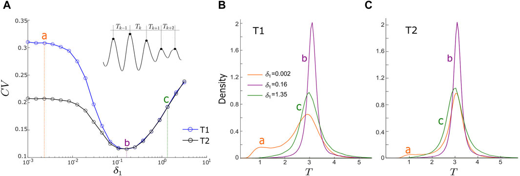
FIGURE 4. (A) Coefficient of variation (CV) vs. noise intensity, δ₁, for motifs T1 (blue curve) and T2 (black curve). (CV) is defined in Eq. 6. Points a, b, and c represent noise intensities of δ₁ = 0.0023 (weak noise), 0.16 (intermediate noise), and 1.35 (strong noise). Panel A inset illustrates period (T_k) calculation. (B,C): density functions of periods (T) for motifs T1 and T2, respectively, with three values of δ₁. Orange, purple and green lines correspond to these three noise intensities labelled as points a, b and c in Panel A. Other parameters are: α = −0.2; ρ = −0.2; ω₀ = 2; ω₁ = 0; δ₂ = δ₃ = 0.01; and λ₀ = −0.1; with d_1,3 = d_2,3 = d_1,2 = 0.1 for motif T1; and d_1,3 = −d_2,3 = d_1,2 = 0.1 for motif T2.

The results of our analysis are presented in Figure 4A, illustrating how CV varies with changes in the driving noise intensity, δ₁, for both the T1 motif (shown as the blue curve) and the T2 motif (represented by the black curve). In both motifs, we observe a resonant pattern: as δ₁ increases, CV firstly experiences a decline, reaching a minimum point before rising again. This suggests that the optimization of noise-induced oscillations in the output node can be achieved at an intermediate δ₁ value.

We observe, however, that motif T1 consistently exhibits higher CV values compared to motif T2 over 0.001 ≤ δ₁ < 0.16 (Figure 4A). This observation suggests that motif T2 exhibits greater output regularity than T1. This observation aligns with our earlier findings in the timeseries and time-averaged amplitude of the output node in Figure 2, where motif T2 demonstrates a higher level of oscillation regularity in its output node relative to motif T1. As δ₁ approaches the optimal point at ${\delta }_1^{*}=0.162$, the gap between these two curves gradually diminishes. Interestingly, both motifs share the identical optimal noise intensity and corresponding minima in CV, denoted CV*. For example, in Figure 4A, we identify ${\delta }_1^{*}=0.162$ and CV* = 0.116 for both motifs T1 and T2. Moreover, as δ₁ continues to increase, the blue and black curves in Figure 4A converge and increase with the increment of δ₁, suggesting that the oscillation regularity induced by relatively strong noise is motif-independent.

The density functions (DFs) of the oscillation periods of the output node within each motif can offer additional insights into the connection between oscillation control and the intensity of the driving noise. We specifically investigated three distinct values of δ₁ (0.0023, 0.16, and 1.35) to represent scenarios of weak, optimal, and strong noise intensities. Significantly, the DFs associated with δ₁ = 0.16 (represented by the purple curves in Figure 4B for motif T1 and Figure 4C for motif T2) exhibit the most prominent features (the highest peaks and the narrowest half-widths) in comparison to the other DFs. This observation implies that, at the optimal noise intensity, the oscillation periods are most tightly clustered around a central value, indicating the highest regularity in the noise-induced oscillations. This observation aligns with the minimum CV at point b in Figure 4A. At a low noise intensity (δ₁ = 0.0023), the DF of motif T2 (orange curve in Figure 4B) exhibits a higher peak and a narrower half-width compared to motif T1’s DF (orange curve in Figure 4C). This observation implies that within the low-intensity range of δ₁, the output of motif T2 displays superior oscillation regularity, corroborating our earlier findings in Figure 2. Under strong noise conditions (δ₁ = 1.35), the DFs of both motifs (green curves in Figures 4B, C) closely resemble each other, indicating that motif structure has minimal influence on oscillations induced by strong noise.

In summary, we observe a trend in which the oscillation regularity of the output in both motifs T1 and T2 is steadily enhanced as noise intensity increases from low levels to a specific optimal point. Prior to reaching this optimum, motif T2 outperforms motif T1, as evidenced by a lower CV. However, beyond this optimal point, the oscillation regularity of both T1 and T2 motifs converges, and with further increases in the intensity of noise, output regularity consistently diminishes.

3.4 The combined effects of noise and intra-motif coupling

In Section 3.2; Section 3.3, we examined the impact of the driving noise intensity, δ₁, on motif synchrony and output regularity while keeping the intra-motif coupling strengths (d_1,3, d_2,3, and d_1,2) constant. Here we investigate the combined influence of intra-motif coupling and noise on motif synchronization and output regularity. For simplicity, we assume that within each motif, the three coupling strengths are identical, represented as d. That is, d_1,3 = d_2,3 = d_1,2 = d in motif T1, and d_1,3 = −d_2,3 = d_1,2 = d in motif T2. The root mean square deviation, σ, in Eq. 4 and the coefficient of variation of periods, CV, in Eq. 7 are used to evaluate motif synchrony and output regularity, respectively. Our findings are demonstrated in Figure 5, which presents contour maps illustrating how σ and CV change as functions of δ₁ and d for both the T1 motif (Figures 5A, B) and the T2 motif (Figures 5C, D). The color bars in these panels serve as a visual reference for the σ and CV values, with colder colors indicating greater motif synchrony and higher output regularity, respectively.

FIGURE 5

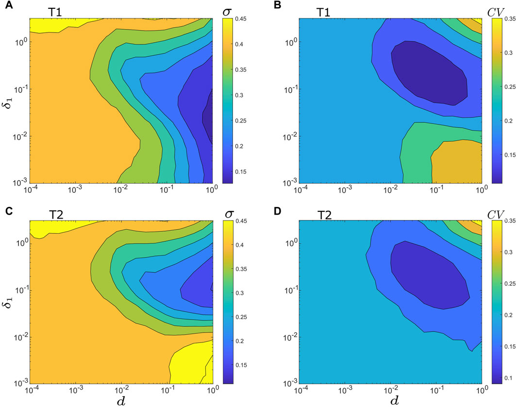
FIGURE 5. Contour maps of σ and CV vs. noise intensity δ₁ vs. intra-motif coupling strength d. (A) σ vs. δ₁ vs. d for motif T1. (B) CV vs. δ₁ vs. d for motif T1. (C) σ vs. δ₁ vs. d for motif T2. (D) CV vs. δ₁ vs. d for motif T2. For (A,B): d = d_1,3 = d_2,3 = d_1,2. For (C,D): d = d_1,3 = −d_2,3 = d_1,2. Other parameters are: α = −0.2; ρ = −0.2; ω₀ = 2; ω₁ = 0; δ₂ = δ₃ = 0.01; and λ₀ = −0.1.

In general, the comparison of noise-induced synchrony of both motifs in Figures 5A, C reveal that motif synchrony is enhanced as the coupling strength (d) increases, and the optimized synchrony is achieved at the intermediate noise intensity. However, an obvious difference emerges for the combination of weak noise (δ₁ < 0.04) and intermediate to strong coupling strength (d > 0.01), as demonstrated in the lower-right sections of Figures 5A, C. In this range, motif T1 shows a stronger tendency toward synchronization, while motif T2 displays a higher degree of asynchrony due to the inhibitory connection between its intermediate and output nodes.

The oscillation regularity of the output node in both motifs, as shown in Figures 5B, D, demonstrates that the optimal output regularity is achieved at intermediate coupling strengths with a slightly strong noise intensity. Specifically, under the current model parameters, the minimum CV is situated at approximately d ≈ 0.05 and δ₁ ≈ 0.2. However, a significant deviation in output regularity can be observed in the lower-right corners of Figures 5B, D, corresponding to δ₁ < 0.02 and d > 0.02. In this specific region, motif T1 exhibits very low output regularity, whereas motif T2 shows relatively better regularity.

It’s important to emphasize that the region of major difference in motif synchrony aligns with this area as well. Therefore, the primary differentiation between motif T1 and T2 emerges in scenarios of low noise intensity but strong coupling, with motif T1 yielding high synchrony but low output regularity, and motif T2 generating low synchrony but relatively high output regularity. Furthermore, it’s worth mentioning that these differences become less prominent when the intra-motif coupling is extremely weak (the left half of each panel in Figure 5) or when there is excessive intrinsic noise and intra-motif coupling (the upper-right region of each panel in Figure 5).

The comprehensive analysis in Figure 5 reveals that the optimal levels of motif synchrony (σ*) and output regularity (CV*) rely on the coupling strength (d). To further explore this dependence, we calculate σ* and CV*, along with their corresponding ${\delta }_1^{*}$ values, as functions of d and display them in Figure 6. Both motifs exhibit a negative correlation between σ* and d (Figure 6A) and an anti-correlation between the associated ${\delta }_1^{*}$ and d (Figure 6C), indicating that, as the coupling strength increases, the level of optimized motif synchrony increases and the required noise intensity to achieve this synchronization decreases. Moreover, CV* derived from both motifs exhibits nearly indistinguishable non-monotonic curves, displaying a declining-then-increasing pattern as d increases (Figure 6B). Both motifs achieve identical optimal output regularity, CV* = 0.108, at d = 0.05. The optimal noise intensity, ${\delta }_1^{*}$, associated with CV* has a negative correlation with d (Figure 6D). These findings indicate that intermediate coupling, rather than strong coupling, optimizes output regularity, and the noise intensity required to maximize regularity decreases as the coupling strength increases, contradicting the anticipated notion that stronger coupling would enhance output regularity.

FIGURE 6

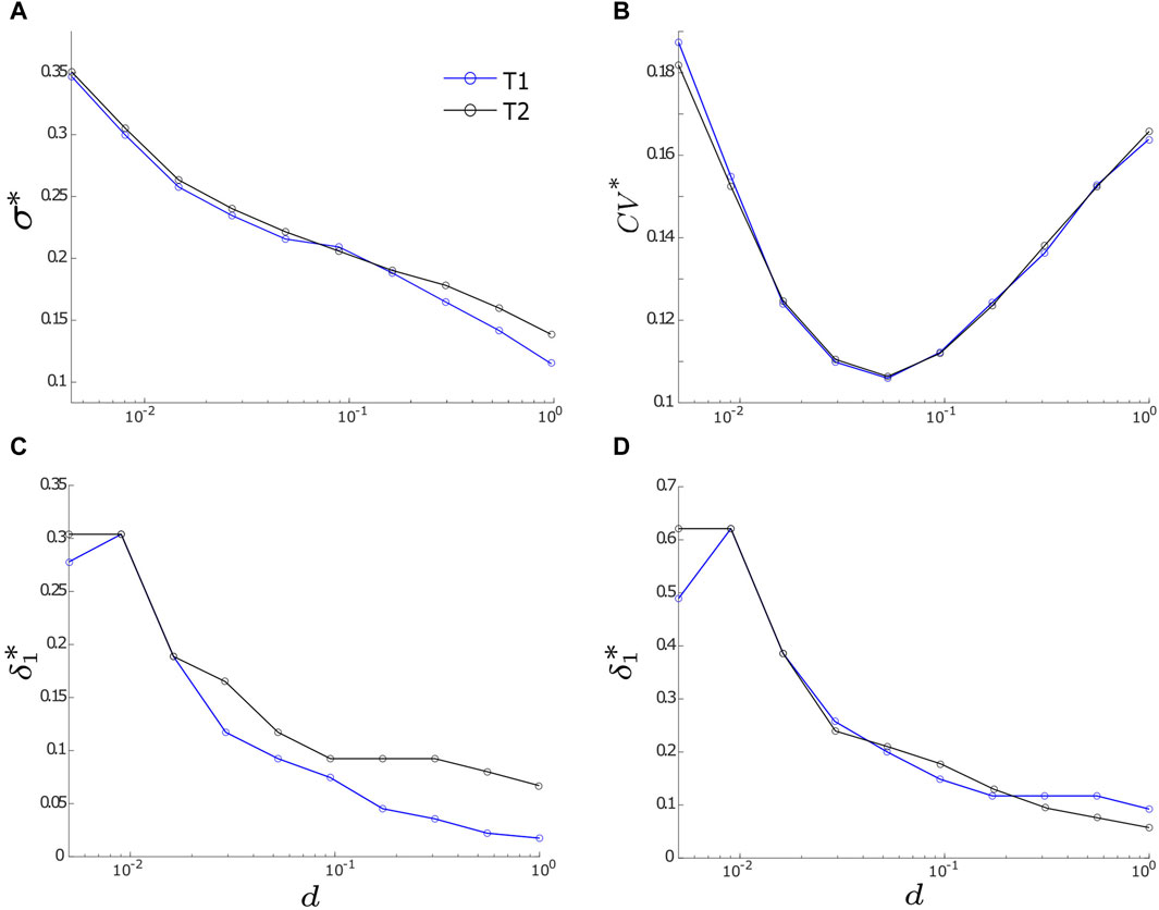
FIGURE 6. The optimal values of σ and CV (denoted as σ* and CV*, respectively) along with their corresponding optimal noise intensities $({\delta }_1^{*})$ are plotted against the equal coupling strength (d). (A,C): σ* and corresponding ${\delta }_1^{*}$ vs. d, respectively. (B,D): CV* and corresponding ${\delta }_1^{*}$ vs. d, respectively. Blue and black curves correspond to motifs T1 and T2, respectively. Other parameters are: α = −0.2; ρ = −0.2; ω₀ = 2; ω₁ = 0; δ₂ = δ₃ = 0.01; λ₀ = −0.1; d = d_1,3 = d_2,3 = d_1,2 for the T1 motif; and d = d_1,3 = −d_2,3 = d_1,2 for the T2 motif.

3.5 The influence of the control parameter of Hopf bifurcation

In our investigation of the noise-induced dynamics of FFL motifs in the previous sections, we have maintained a constant value for the control parameter of HB in the excitable regime, specifically λ₀ = −0.1. However, as λ₀ approaches the critical HB point (λ₀ = 0), there is a gradual increase in the amplitude of noise-induced oscillations [37, 38]. Therefore, we study the impact of varying λ₀ on both motif synchronization and output regularity in this section, recognizing its vital role in predicting and regulating system behavior.

In this analysis, we keep the coupling strength fixed at 0.1 and compute the average values of σ and CV over a noise intensity range of 0.001 ≤ δ₁ ≤ 0.5, denoted as ⟨σ⟩ and ⟨CV⟩, respectively. This averaging calculation is performed for each λ₀ ranging from −1 to −0.001 for both motifs. For each λ₀ value, we also calculate the optimal driving noise intensity, ${\delta }_1^{*}$, required to minimize σ or CV, respectively. The results are illustrated in Figure 7, with the blue curves denoting motif T1 and the black curves representing motif T2.

FIGURE 7

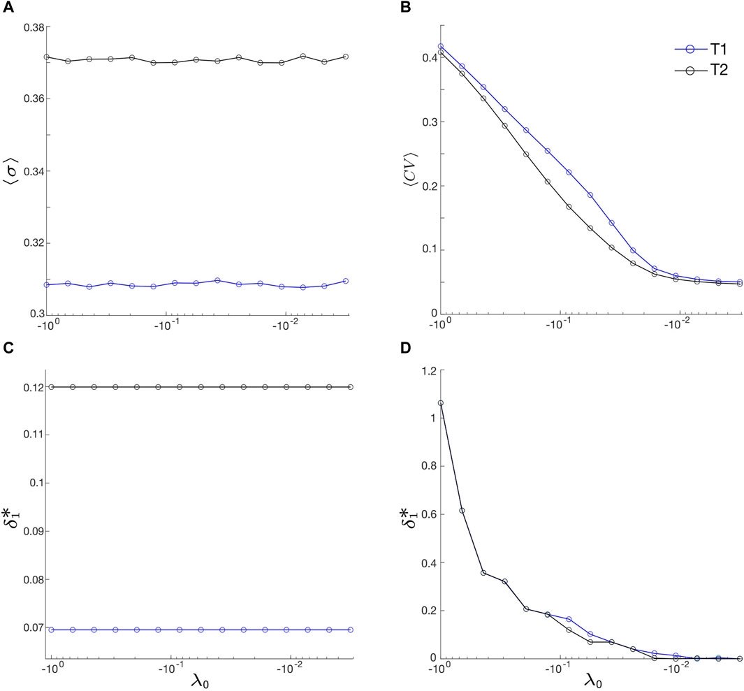
FIGURE 7. (A) Average motif synchronization, ⟨σ⟩, and (B) average output regularity, ⟨CV⟩, vs. λ₀. ⟨σ⟩ and ⟨CV⟩ represent the averages of σ and CV over a noise intensity range of 0.001 ≤ δ₁ ≤ 0.5, respectively. (C,D): ${\delta }_1^{*}$ vs. λ₀. ${\delta }_1^{*}$ denotes the noise intensities required to optimize motif synchronization in panel (A) and output regularity in panel (B), respectively. Blue and black curves represent the T1 and T2 motifs, respectively. Other parameters are: α = −0.2, ρ = −0.2, ω₀ = 2, ω₁ = 0, δ₂ = δ₃ = 0.01, d_1,3 = d_2,3 = d_1,2 = 0.1 for motif T1, and d_1,3 = −d_2,3 = d_1,2 = 0.1 for motif T2.

Surprisingly, we find that ⟨σ⟩ appears constant (Figure 7A), with ⟨σ⟩ ≈ 0.308 for motif T1 and about 0.372 for motif T2. Meanwhile, ${\delta }_1^{*}$ required to minimize σ is also constant for each motif (${\delta }_1^{*}\approx 0.07$ for motif T1 motif and approximately 0.12 for motif T2) as shown in Figure 7C. This suggests that motif synchronization and its corresponding optimal noise intensity remains unaffected by the proximity of λ₀ to the critical HB point. Furthermore, Figure 7A shows that ⟨σ⟩ is consistently lower for motif T1 compared to motif T2. Figure 7C displays the same trend in ${\delta }_1^{*}$, with ${\delta }_1^{*}$ consistently being lower in motif T1 than in motif T2. This agrees with our earlier findings in Figures 6A, C. These results imply that, on average, within the excitable range of −1 ≤ λ₀ ≤ −0.08, motif T1 requires a relatively lower optimal noise intensity to attain a relatively higher level of synchrony than motif T2.

On the other hand, Figures 7B, D demonstrate a robust inverse relationships between ⟨CV⟩ and λ₀ and between ${\delta }_1^{*}$ and λ₀, respectively, for both motifs. We observe a near-linear reduction in ⟨CV⟩ as λ₀ approaches the HB point (λ₀ = 0) for both motifs, although motif T2 exhibits slightly lower values than motif T1 (Figure 7B). However, the corresponding ${\delta }_1^{*}$ are roughly equivalent for both motifs (Figure 7D). This suggests that, on average, within the excitable range, the noise-induced oscillations produced by motif T2’s output node demonstrate a higher level of regularity compared to motif T1. This observation aligns with our findings from the timeseries depicted in Figures 2B, E, as well as the behavior of CV illustrated in Figure 4A.

4 Discussion

In summary, this study demonstrates that both coherent and incoherent FFL motifs exhibit resonance patterns in terms of network motif synchrony and output regularity, that is, motif synchrony and output regularity reach their optimal levels at the intermediate noise intensities. This aligns with previous studies in analogous networks, which have reported on the existence of coherence resonance and other phenomena related to “stochastic facilitation” [39], such as in [40–43].

We have uncovered distinct functional characteristics within the two FFL motifs. The coherent motif (motif T1), characterized by purely excitatory connections, displays a higher level of noise-induced synchronization and requires lower noise intensities to achieve maximum synchrony. In contrast, the incoherent motif (motif T2), distinguished by an inhibitory connection from the intermediate layer to the output layer, excels in output regularity. This implies that changing the excitatory coupling between the intermediate and output nodes (or layers) of the FFL to inhibitory coupling, essentially transitioning from a coherent to an incoherent FFL, promotes output regularity but reduces motif synchrony. This shift towards inhibitory connectivity reveals a trade-off between motif synchrony and output regularity, suggesting that the intermediate node (or layer) plays a critical role in shaping the motif’s overall dynamics.

Our study unveils two novel observations. Firstly, we find that the optimal output regularity for both motifs occurs at an intermediate level of intra-motif coupling (Figures 5B, D), challenging the common expectation that stronger coupling, especially excitatory coupling, leads to improved regularity. Secondly, as the system approaches the HB point, both motifs exhibit increasingly superior output regularity (Figure 7B), while their motif synchrony and associated optimal noise intensity remain relatively unchanged (Figures 7A, C). These novel findings provide valuable contributions to the study of network motifs.

Our findings indicate that intra-motif coupling exhibits a positive correlation with noise-induced motif synchronization (Figure 6A), but demonstrates a negative correlation with the optimal noise intensity required to maximize synchronization (Figure 6C). These results are in accordance with prior research, underscoring the pivotal role of network connections in shaping network synchrony (e.g., [26, 27, 40, 41, 44]). Considering that FFL motifs play a crucial role in transmitting information from sensory components to effectors in the realm of neuroscience [3, 14], this discovery suggests that motif T2 might serve as a more efficient motif for processing or transmitting information in a noisy environment, which is a pertinent consideration in studies of computational neuroscience. This paper focuses on two common three-node motifs (T1 and T2), highlighting their responses to noise. However, further investigation is needed to develop a comprehensive theory describing the noise-induced dynamics of various three-node motifs. Understanding these dynamics is challenging due to phenomena such as synchrony breaking HB [45, 46], which can occur even without noise. Our future research aims to address these complexities and provide deeper insights into the dynamics of three-node motifs.

Data availability statement

The original contributions presented in the study are included in the article/Supplementary material, further inquiries can be directed to the corresponding author.

Author contributions

GJ: Conceptualization, Formal Analysis, Investigation, Methodology, Software, Visualization, Writing–original draft, Writing–review and editing. NY: Conceptualization, Formal Analysis, Investigation, Methodology, Supervision, Writing–original draft, Writing–review and editing, Visualization. YL: Writing–review and editing.

Funding

The author(s) declare that financial support was received for the research, authorship, and/or publication of this article. GJ is supported by the Queen Elizabeth II Graduate Scholarship in Science and Technology and the Ontario Graduate Scholarship in Canada. NY and YL received startup funding from the Faculty of Science at Toronto Metropolitan University and the Discovery Grant from the Natural Sciences and Engineering Research Council of Canada (NSERC).

Conflict of interest

The authors declare that the research was conducted in the absence of any commercial or financial relationships that could be construed as a potential conflict of interest.

Publisher’s note

All claims expressed in this article are solely those of the authors and do not necessarily represent those of their affiliated organizations, or those of the publisher, the editors and the reviewers. Any product that may be evaluated in this article, or claim that may be made by its manufacturer, is not guaranteed or endorsed by the publisher.

References

1. Mangan S, Alon U. Structure and function of the feed-forward loop network motif. Proc Natl Acad Sci USA (2003) 100:11980–5. doi:10.1073/pnas.2133841100

PubMed Abstract | CrossRef Full Text | Google Scholar

2. Alon U. Network motifs: theory and experimental approaches. Nat Rev Genet (2007) 8:450–61. doi:10.1038/nrg2102

PubMed Abstract | CrossRef Full Text | Google Scholar

3. Milo R, Shen-Orr S, Itzkovitz S, Kashtan N, Chklovskii D, Alon U. Network motifs: simple building blocks of complex networks. Science (2002) 298:824–7. doi:10.1126/science.298.5594.824

PubMed Abstract | CrossRef Full Text | Google Scholar

4. Reigl M, Alon U, Chklovskii DB. Search for computational modules in the c. elegans brain. BMC Biol (2004) 2:25. doi:10.1186/1741-7007-2-25

PubMed Abstract | CrossRef Full Text | Google Scholar

5. Song S, Sjöström PJ, Reigl M, Nelson S, Chklovskii DB. Highly nonrandom features of synaptic connectivity in local cortical circuits. PLoS Biol (2005) 3:e68. doi:10.1371/journal.pbio.0030068

PubMed Abstract | CrossRef Full Text | Google Scholar

6. Shen-Orr S, Milo R, Mangan S, Alon U. Network motifs in the transcriptional regulation network of escherichia coli. Nat Genet (2002) 31:64–8. doi:10.1038/ng881

PubMed Abstract | CrossRef Full Text | Google Scholar

7. Lee TI, Rinaldi NJ, Robert F, Odom DT, Bar-Joseph Z, Gerber GK, et al. Transcriptional regulatory networks in Saccharomyces cerevisiae. Science (2002) 298:799–804. doi:10.1126/science.1075090

PubMed Abstract | CrossRef Full Text | Google Scholar

8. Wuchty S, Oltvai ZN, Barabási AL. Evolutionary conservation of motif constituents in the yeast protein interaction network. Nat Genet (2003) 35:176–9. doi:10.1038/ng1242

PubMed Abstract | CrossRef Full Text | Google Scholar

9. Boyer LA, Lee TI, Cole MF, Johnstone SE, Levine SS, Zucker JP, et al. Core transcriptional regulatory circuitry in human embryonic stem cells. Cell (2005) 122:947–56. doi:10.1016/j.cell.2005.08.020

PubMed Abstract | CrossRef Full Text | Google Scholar

10. Tsang J, Zhu J, van Oudenaarden A. MicroRNA-mediated feedback and feedforward loops are recurrent network motifs in mammals. Mol Cel (2007) 26:753–67. doi:10.1016/j.molcel.2007.05.018

PubMed Abstract | CrossRef Full Text | Google Scholar

11. Sporns O, Kötter R. Motifs in brain networks. PLoS Biol (2004) 2:e369. doi:10.1371/journal.pbio.0020369

PubMed Abstract | CrossRef Full Text | Google Scholar

12. Eggermont J. Representation of spectral and temporal sound features in three cortical fields of the cat. Similarities outweigh differences. J Neurophysiol (1998) 80:2743–64. doi:10.1152/jn.1998.80.5.2743

PubMed Abstract | CrossRef Full Text | Google Scholar

13. Middleton JW, Longtin A, Benda J, Maler L. The cellular basis for parallel neural transmission of a high-frequency stimulus and its low-frequency envelope. Proc Natl Acad Sci (2006) 103:14596–601. doi:10.1073/pnas.0604103103

PubMed Abstract | CrossRef Full Text | Google Scholar

14. Macía J, Widder S, Solé R. Specialized or flexible feed-forward loop motifs: a question of topology. BMC Syst Biol 3 (2009) 84. doi:10.1186/1752-0509-3-84

PubMed Abstract | CrossRef Full Text | Google Scholar

15. Varela F, Lachaux JP, Rodriguez E, Martinerie J. The brainweb: phase synchronization and large-scale integration. Nat Rev Neurosci (2001) 2:229–39. doi:10.1038/35067550

PubMed Abstract | CrossRef Full Text | Google Scholar

16. Buzsáki G. Rhythms of the brain. United Kingdom: Oxford Academic (2006). doi:10.1093/acprof:oso/9780195301069.001.0001

CrossRef Full Text | Google Scholar

17. Arkady P, Michael R, Jürgen J. Synchronization: a universal concept in nonlinear sciences. Cambridge: Cambridge University Press (2003).

Google Scholar

18. Steven HS. Sync: the emerging science of spontaneous order. United States: Hachette Books (2003).

Google Scholar

19. Elbert BR. Introduction to satellite communication. United States: Artechhouse (2008).

Google Scholar

20. Sobot R. Wireless communication electronics: introduction to RF circuits and design techniques. Berlin, Germany: Springer Science and Business Media (2021). doi:10.1007/978-3-030-48630-3

CrossRef Full Text | Google Scholar

21. Wiesenfeld MFK, Moss F. Stochastic resonance and the benefits of noise: from ice ages to crayfish and squids. Nature (1995) 373:33–6. doi:10.1038/373033a0

PubMed Abstract | CrossRef Full Text | Google Scholar

22. Faisal AA, Selen LP, Wolpert DM. Noise in the nervous system. Nat Rev Neurosci (2008) 9:292–303. doi:10.1038/nrn2258

PubMed Abstract | CrossRef Full Text | Google Scholar

23. Gui R, Liu Q, Yao Y, Deng H, Ma C, Jia Y, et al. Noise decomposition principle in a coherent feed-forward transcriptional regulatory loop. Front Physiol (2016) 7:600. doi:10.3389/fphys.2016.00600

PubMed Abstract | CrossRef Full Text | Google Scholar

24. Krauss P, Prebeck K, Schilling A, Metzner C. Recurrence resonance in three-neuron motifs. Front Comput Neurosci (2019) 13:64. doi:10.3389/fncom.2019.00064

PubMed Abstract | CrossRef Full Text | Google Scholar

25. Bönsel F, Krauss P, Metzner C, Yamakou ME. Control of noise-induced coherent oscillations in three-neuron motifs. Cogn Neurodyn (2022) 16:941–60. doi:10.1007/s11571-021-09770-2

PubMed Abstract | CrossRef Full Text | Google Scholar

26. Yu N, Kuske R, Li Y. Stochastic phase dynamics: multiscale behavior and coherence measures. Phys Rev E (2006) 73:056205. doi:10.1103/PhysRevE.73.056205

PubMed Abstract | CrossRef Full Text | Google Scholar

27. Jagdev G, Yu N. Noise-induced synchrony of two-neuron motifs with asymmetric noise and uneven coupling. Front Comput Neurosci (2024) 18:1347748. doi:10.3389/fncom.2024.1347748

CrossRef Full Text | Google Scholar

28. Wang Q, Perc M, Duan Z, Chen G. Synchronization transitions on scale-free neuronal networks due to finite information transmission delays. Phys Rev E (2009) 80:026206. doi:10.1103/PhysRevE.80.026206

PubMed Abstract | CrossRef Full Text | Google Scholar

29. Gao Z, Hu B, Hu G. Stochastic resonance of small-world networks. Phys Rev E (2001) 65:016209. doi:10.1103/PhysRevE.65.016209

PubMed Abstract | CrossRef Full Text | Google Scholar

30. Rosenblum M, Pikovsky A, Kurths J, Schäfer C, Tass PA. Chapter 9 Phase synchronization: from theory to data analysis. Handbook Biol Phys (2001) 4:279–321. doi:10.1016/S1383-8121(01)80012-9

CrossRef Full Text | Google Scholar

31. Gang H, Ditzinger T, Ning CZ, Haken H. Stochastic resonance without external periodic force. Phys Rev Lett (1993) 71:807–10. doi:10.1103/PhysRevLett.71.807

PubMed Abstract | CrossRef Full Text | Google Scholar

32. Pikovsky AS, Kurths J. Coherence resonance in a noise-driven excitable system. Phys Rev Lett (1997) 78:775–8. doi:10.1103/PhysRevLett.78.775

CrossRef Full Text | Google Scholar

33. Mormann F, Lehnertz K, David P, Elger CE. Mean phase coherence as a measure for phase synchronization and its application to the eeg of epilepsy patients. Physica D: Nonlinear Phenomena (2000) 144:358–69. doi:10.1016/S0167-2789(00)00087-7

CrossRef Full Text | Google Scholar

34. Lindner B, Schimansky-Geier L, Longtin A. Maximizing spike train coherence or incoherence in the leaky integrate-and-fire model. Phys Rev E (2002) 66:031916. doi:10.1103/PhysRevE.66.031916

PubMed Abstract | CrossRef Full Text | Google Scholar

35. Lu L, Bao C, Ge M, Xu Y, Yang L, Zhan X, et al. Phase noise-induced coherence resonance in three dimension memristive hindmarsh-rose neuron model. Eur Phys J Spec Top (2019) 228:2101–10. doi:10.1140/epjst/e2019-900011-1

CrossRef Full Text | Google Scholar

36. Bönsel F, Krauss P, Metzner C, Yamakou ME. Control of noise-induced coherent oscillations in three-neuron motifs. Cogn Neurodynamics (2022) 16:941–60. doi:10.1007/s11571-021-09770-2

CrossRef Full Text | Google Scholar

37. Yu G, Yi M, Jia Y, Tang J. A constructive role of internal noise on coherence resonance induced by external noise in a calcium oscillation system. Chaos, Solitons & Fractals (2009) 41:273–83. doi:10.1016/j.chaos.2007.12.001

CrossRef Full Text | Google Scholar

38. Yu N, Jagdev G, Morgovsky M. Noise-induced network bursts and coherence in a calcium-mediated neural network. Heliyon (2021) 7:e08612. doi:10.1016/j.heliyon.2021.e08612

PubMed Abstract | CrossRef Full Text | Google Scholar

39. McDonnell MD, Ward LM. The benefits of noise in neural systems: bridging theory and experiment. Nat Rev Neurosci (2011) 12:415–25. doi:10.1038/nrn3061

PubMed Abstract | CrossRef Full Text | Google Scholar

40. Lu L, Jia Y, Kirunda JB, Xu Y, Ge M, Pei Q, et al. Effects of noise and synaptic weight on propagation of subthreshold excitatory postsynaptic current signal in a feed-forward neural network. Nonlinear Dyn (2019) 95:1673–86. doi:10.1007/s11071-018-4652-9

CrossRef Full Text | Google Scholar

41. Guo D, Li C. Stochastic and coherence resonance in feed-forward-loop neuronal network motifs. Phys Rev E (2009) 79:051921. doi:10.1103/PhysRevE.79.051921

PubMed Abstract | CrossRef Full Text | Google Scholar

42. Lou X. Stochastic resonance in neuronal network motifs with ornstein-uhlenbeck colored noise. Math Probl Eng (2014) 2014:1–7. doi:10.1155/2014/902395

CrossRef Full Text | Google Scholar

43. Krauss P, Prebeck K, Schilling A, Metzner C. Recurrence resonance in three-neuron motifs. Front Comput Neurosci (2019) 13:64. doi:10.3389/fncom.2019.00064

PubMed Abstract | CrossRef Full Text | Google Scholar

44. Ge M, Jia Y, Lu L, Xu Y, Wang H, Zhao Y. Propagation characteristics of weak signal in feedforward izhikevich neural networks. Nonlinear Dyn (2020) 99:2355–67. doi:10.1007/s11071-019-05392-w

CrossRef Full Text | Google Scholar

45. Golubitsky M, Postlethwaite C. Feed-forward networks, center manifolds, and forcing. Discrete Continuous Dynamical Syst (2012) 32:2913–35. doi:10.3934/dcds.2012.32.2913

CrossRef Full Text | Google Scholar

46. Rink B, Sanders J. Amplified hopf bifurcations in feed-forward networks. SIAM J Appl Dynamical Syst (2013) 12:1135–57. doi:10.1137/120899649

CrossRef Full Text | Google Scholar