Dimensionality reduction and machine learning based model of software cost estimation

Software Cost Estimation (SCE) is one of the research priorities and challenges in the construction of cyber-physical-social systems (CPSSs). In CPSS, it is urge to process environmental and social information accurately and use it to guide social practice. Thus, in response to the problems of low prediction accuracy, poor robustness, and poor interpretability in SCE, this paper proposes a SCE model based on Autoencoder and Random Forest. First, preprocess the project data, remove outliers, and build regression trees to fill in missing attributes in the data. Second, construct a Autoencoder to reduce the dimensionality of factors that affect software cost. Subsequently, the performance of the model was trained and validated using the XGBoost framework on three datasets: COCOMO81, Albrecht, and Desharnais, and compared with common cost prediction models. The experimental results show that the MMRE, MdMRE, and PRED (0.25) values of the proposed model on the COCOMO81 dataset reached 0.21, 0.16, and 0.71, respectively. Compared with other models, the proposed model achieved significant improvements in accuracy and robustness.

1 Introduction

In the era of big data, the new paradigm of computer-based platforms and people-oriented approaches has gradually demonstrated its strong vitality and potential value, triggering a new form of research on complex system modeling, analysis, control, and management, which is known as cyber-physical-social systems (CPSSs). One of the main issues in CPSS research is how to use data as a guide and construct accurate models to regulate social relationships between people, which is also an important issue in software engineering research. As a part of software engineering, Software Cost Estimation (SCE) not only needs to collect and analyze multi-dimensional information about software development needs, but also needs to consider the team’s collaborative ability and personnel management costs [1–4]. The predicted results generated through computer algorithms will provide managers with unprecedented efficient management capabilities and improve the team’s resource allocation efficiency, building an efficient communication bridge between engineering development and personnel management, thus improving the quality of software development and reducing the risk of research and development failure. Therefore, how to accurately predict the costs of software development has been one of the most important topics studied in software engineering in recent years [5, 6].

However, in practical applications, due to the large number of indicators used for project evaluation and unclear functional requirements in the early stages of development, managers can hardly accurately predict the cost of software development in most cases, resulting in erroneous decisions and unnecessary losses for the company. In addition, with the continuous development of software development technology, object-oriented programming has become the dominant paradigm of software development. Object-oriented design principles such as the single responsibility principle, low coupling, and high cohesion also increase the difficulty of cost estimation [7]. The long development cycle of large-scale software engineering, the significant differences between different projects, and the limited availability of previous project data for cost evaluation hinder the feature learning and data fitting of the constructed model, further limiting the accuracy of the results.

In the process of software development, many cost estimation tasks are completed manually by managers. However, with the expansion of software engineering, the difficulty of implementing this method and the accuracy of the results are unsatisfactory. Therefore, many studies have proposed more automated and intelligent techniques to complete this task. Esteve and Aparicio [8] used the ID3 algorithm to generate a large number of decision trees to classify software modules with high development intensity. In [9], the author studied the application of fuzzy ID3 decision tree. This method is designed by combining the concepts of ID3 algorithm and fuzzy set theory, and uses MMRE and Pred as the criteria for measuring prediction accuracy. The above algorithms all use weak classifiers or regressors to generate prediction models. Although the convergence speed of the models are fast, due to the large differences in mathematical features between different projects, the robustness of the models are poor, making them difficult to obtain reliable prediction results [10, 11]. While deep learning based methods can explore the potential correlations between various attributes better, they require a large amount of data to train the weights of neural networks. Considering the small size of the dataset used in SCE, the model obtained by this method cannot converge well, resulting in low prediction accuracy [12].

To improve the problem of low prediction accuracy and insufficient model robustness in SCE, this paper proposes a SCE model based on Autoencoder and Random Forest. By using neural networks to non-linearly recombine some attributes, various factors that affect software cost are comprehensively reflected from different perspectives, making the new attributes have stronger interpretability and reduce the losses in the final prediction results due to deviations in some attribute values. At the same time, using the Random Forest model to achieve SCE avoids the problem of low model accuracy caused by insufficient data sets, resulting in a model with strong generalization and robustness, which can achieve more reliable prediction results in practical applications.

2 Theory and methods

2.1 Dimensionality reduction

Usually, several attributes are used to describe different characteristics of the projects from multiple dimensions in SCE. Richer dimensional information can more comprehensively characterize the cost of a project and improve the accuracy of predictions, but to some extent it also increases the difficulty of data collection, making the prediction results vulnerable to noise [13]. In addition, there may be strong correlations among attributes, resulting in certain attributes affecting the result of prediction together from a single dimension, reducing the robustness and interpretability of the model. To solve this problem, we will use dimensionality reduction method on the original data, reorganizing some variables with complex relationships into a few comprehensive factors, so that the recombined factors can reflect the cost of software development from different perspectives, avoiding the problem of low model accuracy caused by large estimation bias of single attribute.

Principal Component Analysis and Factor Analysis methods have been widely applied in the field of software engineering [14, 15]. However, as linear dimensionality reduction methods, they often fail to achieve good dimensionality reduction effects in scenarios where complex data and high data structure preservation requirements are present. In recent years, with the widespread application of artificial neural networks in the field of data dimensionality reduction [16, 17], Autoencoder, as a nonlinear dimensionality reduction method, can more accurately identify and reorganize data attributes, fully explore the potential correlations between data, and has strong anti-interference ability for noise in data, which is suitable for dimensionality reduction of data in software engineering [18, 19]. The Autoencoder used for dimensionality reduction only contains the encoding part, which consists of an input layer, several hidden layers, and an output layer. Its structure is shown in Figure 1. In the encoder, input data is passed through a series of hidden layers for transformation and mapping to the output layer. Each hidden layer consists of multiple neurons, each of which is connected to neurons in the previous layer and undergoes nonlinear transformation through an activation function. The goal of the encoder is to learn an encoding function that maps input data to a low-dimensional representation in the encoding layer. This encoding process is usually achieved through optimization methods such as backpropagation and gradient descent. By adjusting the network’s weights and biases, the encoder gradually learns a set of features that can effectively represent the input data. The training process of Autoencoder usually uses unsupervised learning methods, which only use the input data itself without requiring label information. This allows Autoencoder to be trained on unlabeled data, thereby better adapting to the complex data distribution in software engineering.

FIGURE 1

FIGURE 1. Structure of the Autoencoder uesd for dimensionality reduction.

2.2 Random forest model

At present, existing prediction models mainly include methods based on the function point method and neural network-based methods. The prediction results of the former are more subjective and have lower prediction accuracy, because in the early stages of a project, there is usually only a user requirement document, lacking a complete software system specification document. Neural network-based evaluation methods require a large amount of sample data to train the neural network, but historical SCE data is often limited, resulting in models that cannot converge to good results. In addition, the poor interpretability of deep learning models is not conducive to evaluating the quality and stability of the model. To achieve the desired prediction accuracy and convergence speed, we used a Random Forest model to implement the task. Considering that historical data is often limited in practical applications, we adopted the XGBoost algorithm framework to build the model to accelerate the model’s convergence process.

The XGBoost algorithm [20] uses second-order Taylor expansion to calculate the loss function, adds a regularization term to the GBDT objective function, and uses first and second-order derivatives to approximate the objective function. This approach simplifies the model and effectively reducing the risk of overfitting. The objective function of XGBoost consists of two parts: the loss function and the regularization term:

$L\left(\varphi \right)={\displaystyle \sum _{i=1}^n}l\left(\widehat{y_i},y_i\right)+{\displaystyle \sum _{k=1}^K}\mathrm{\Omega }\left(f_k\right)$

Where $i$ represents the $i$ th sample in the dataset, $n$ is the total number of samples, and $k$ represents the $k$ th regression tree. $l\left(\widehat{y_i},y_i\right)$ represents a traditional differentiable convex loss function, which measures the difference between the true label and the predicted label. $\mathrm{\Omega }\left(f_k\right)$ is a regularization term that helps smooth learning weights and avoid overfitting the model. Its calculation formula is as follows:

$\mathrm{\Omega }\left(f\right)=\gamma T+\frac{1}{2}\lambda {‖w‖}^2$

$\gamma$ and $\lambda$ are the regularization parameters, $w$ is the weight vector of the leaf node. When the regularization parameter is set to zero, it becomes a traditional gradient boosting tree.

Since all CART trees are binary trees, the difference between the objective function and the structural score after branching in the algorithm can be measured using the following formula:

$Gain=\frac{1}{2}\left[\frac{G_L^2}{H_L+\lambda }+\frac{G_R^2}{H_R+\lambda }\right.\left.-\frac{{\left(G_L+G_R\right)}^2}{H_L+H_R+\lambda }\right]-\gamma$

$\gamma$ is a punishment item. $G_L$ and $H_L$ are calculated from the left child node, $G_R$ and $H_R$ are calculated from the right child node. $\left(G_L+G_R\right)$ and $\left(H_L+H_R\right)$ are calculated through intermediate nodes.

As a tree model, XGBoost simplifies the modeling process while preserving as much original data information as possible. This algorithm performs well in regression tasks, with higher fitting accuracy, robustness, and generalization ability than other traditional machine learning regression algorithms, and is widely used in data prediction tasks. Therefore, in the practical application of SCE, even with fewer training samples, a model with high prediction accuracy can still be obtained from XGBoost algorithm.

3 Model building strategy based on XGBoost

3.1 Framework of the model

Figure 2 shows the framework of the SCE model proposed in this article, including data preprocessing, XGBoost-based prediction model training, cost prediction, and prediction result analysis stages. The specific process is as follows:

1) Project data preprocessing stage. Clean the data, remove abnormal values from the data, and fill in missing attributes; The Autoencoder is used to reduce the dimensionality of the cleaned data and eliminate redundant information in the dataset. Finally, normalize the data to unify the dimensions of different features.

2) Model training stage. Use the preprocessed data to train the XGBoost Random Forest model. After training reaches the maximum iteration number, the optimal prediction model is output.

3) Software cost prediction stage. Input the data to be evaluated into the model to generate the predicted cost value.

4) Prediction result analysis stage. Determine whether the error of the prediction result is within an acceptable range, convert the numerical value of the result to different levels, and use the results in subsequent software development evaluations.

FIGURE 2

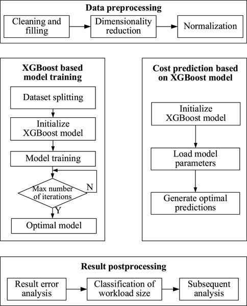
FIGURE 2. Framework of our SCE model.

3.2 Data preprocessing

In practical applications, some data attributes used for software cost evaluation may have missing values or significant deviations from the true values, which can affect the accuracy of the prediction results. To solve this problem, we use the box plot method to remove outliers from the data to avoid the impact of extreme values on the prediction results. Then for all missing values, we use a linear regression tree model to fill them in. Specifically, we select an attribute with missing values as the dependent variable and other attributes as the independent variables to construct a regression tree model. We use the constructed regression tree model to predict the values of missing values, and repeat this step until all missing values are filled.

Then, the Autoencoder is used to reduce the dimensionality of the cleaned data. By using neural networks to transform high-dimensional data into a new low-dimensional coordinate system, the purpose of eliminating redundant information in the data is achieved. If the reduced-dimensional data has too many factors, it will make the model more susceptible to noise and reduce its robustness. On the other hand, having too few factors will lead to a low expression rate of the data and prevent the effective extraction of potential information from the original data. Therefore, we determined the optimal number of factors based on the scree plot in factor analysis and the practical significance of SCE, and the final reduced-dimensional data contained six dimensions, as shown in Figure 3.

FIGURE 3

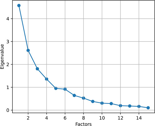
FIGURE 3. Scree plot uesd to determine the number of dimensions.

3.3 Model training

After completing data preprocessing, each data sample will consist of six independent variables and one dependent variable, which is the actual cost value. Predicting the cost of software is essentially finding the mapping relationship between independent variables and dependent variables. To enhance the accuracy and robustness of the model, we will construct several linear regression trees and use gbtree as a booster to construct a Random Forest model. First, shuffle the dataset and split it into a training set and a testing set. Then, generate the optimal model using the training dataset. The specific algorithm is shown in Table 1. After generating the model, the test dataset will be used to evaluate the effectiveness of the model. By comparing the gap between the true value and the model’s estimated value, it can be determined whether the model has overfitting and whether the prediction error is within an acceptable range.

TABLE 1

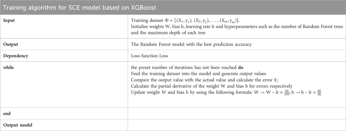
TABLE 1. Model training algorithm steps based on XGBoost.

3.4 Model prediction

After the training of the Random Forest model based on XGBoost, a mapping relationship between factors that affect software cost and the value of that is established, thus providing the ability to assess future software engineering cost. The relevant attributes of the new software engineering project are passed into the model, and after data cleaning and filling, dimensionality reduction and normalization, a column vector with 6 factors is obtained. By inputting it into the trained Random Forest model, the predicted cost value can be obtained.

3.5 Result postprocessing

In order to use the obtained prediction results to guide the actual software development work, we also need to further analyze and process the results. In practical software development, in order to reduce the risk of project failure caused by excessive deviation in cost estimation, it is necessary to further provide a confidence interval for the prediction results, with a confidence level generally taken as 0.80. If the confidence interval is too large, it indicates that the reliability of the results obtained by using this model to predict is poor, and other methods should be used for prediction. If the confidence interval size is within a reasonable range, it indicates that the model’s prediction effect is good. At this point, in order to highlight the practical significance of the prediction effect, the specific numerical value can be converted into five levels (very low, low, moderate, high, very high) to represent different cost extents. Finally, the prediction results will be handed over to the project managers to guide the subsequent software development work.

4 Results and analysis

4.1 Dataset introduction and preprocessing

To verify the effectiveness of the model on different datasets, we will use three different datasets to test the accuracy of the model, namely, COCOMO81, Albrecht, and Desharnais. The COCOMO81 dataset [21] is one of the most popular datasets for SCE, containing data from 63 projects. Each project contains 17 attributes, 15 of which are independent variables and 2 of which are actual cost sizes. The Albrecht dataset contains data from 24 projects implemented by the IBM DP Services organization. These data include the count of four types of external input/output elements of the entire software application, the number of Source Lines Of Code (SLOC) including annotations, and the number of functional points per project; The Desharnais dataset consists of data from 81 software projects at a Canadian software company. These 81 projects are subdivided into 46 projects in traditional environments, 25 projects that “improve” traditional environments, and 10 projects in micro-environments based on their technical environments. It is one of the most classic datasets that can be used for SCE.

The preprocessing of the three datasets includes outlier removal, missing value filling, data dimensionality reduction, and normalization. After analysis using the box plot method, 7 attribute values from COCOMO81, 3 attribute values from Albrecht, and 4 attribute values from Desharnais were eliminated. Then, linear regression tree models were built on the three datasets to predict the removed outliers and original missing values. Then, a correlation analysis was conducted on the datasets, as shown in Figure 4. There was a strong data correlation between the attributes of the three datasets, making it suitable for using Autoencoder for data dimensionality reduction. The hidden layer of the Autoencoder contains three fully connected layers. The first layer contains 20 neurons, the second layer contains 30 neurons, and the third layer contains 10 neurons. The activation function after each layer uses ReLu, and the output layer contains 6 neurons, meaning that the output data contains six dimensions. Finally, the dimension-reduced data is normalized using the Sigmoid function.

FIGURE 4

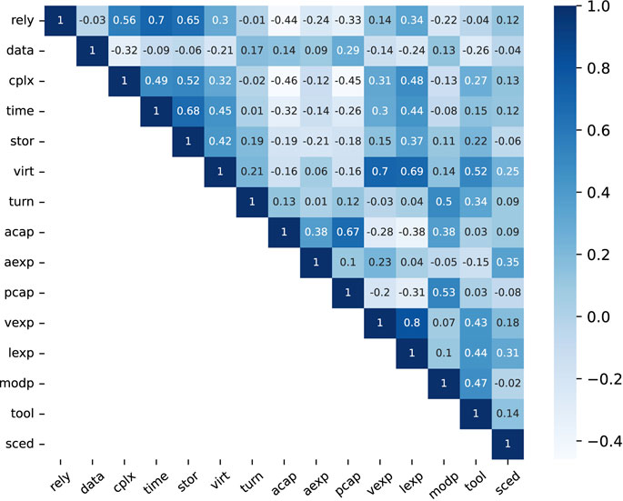
FIGURE 4. Covariance thermogram of various attributes in the COCOMO81 dataset.

4.2 Model training

To ensure that the model can fully converge, we divide the dataset into a training set and a testing set, with the training set accounting for 90% and the testing set accounting for 10%. For the training set data, we use the XGBoost distributed gradient boosting framework to train the model. In order to determine the parameters that can generate the best Random Forest, this experiment uses the method of adjusting hyperparameters rather than theoretical analysis. During the hyperparameter tuning process, different parameter value combinations are used to establish Random Forest models. Then, the parameters that generate the best predictive model are considered to be the most appropriate hyperparameters for that model. The hyperparameters obtained for each model are shown in Table 2.

TABLE 2

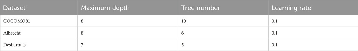
TABLE 2. Performance of the model on different datasets.

4.3 Evaluation criteria in SCE

This article will use three indicators, MMRE, MdMRE, and PRED to evaluate the model [22]. The calculation methods and their meanings of each indicator are shown in Table 3, all of which are based on the Magnitude of Relative Error (MRE):

$MRE=\frac{\left|act-est\right|}{act}$

TABLE 3

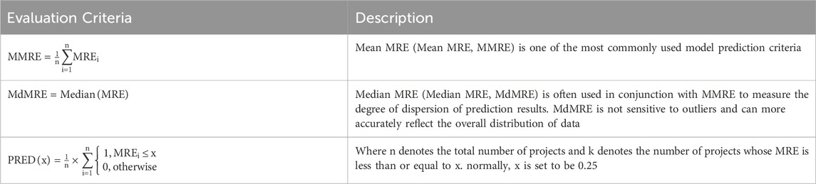
TABLE 3. Model evaluation indicators and their meanings.

Where $act$ represents the actual software cost and $est$ represents the software cost predicted by the model.

4.4 Evaluation and discussion

The performance of the model trained by using the Autoencoder and Random Forest methods on the three test sets is shown in Table 4. As can be seen from the results, the difference between the MMRE and MdMRE indicators for different data sets is quite small, indicating that the prediction results are relatively stable, with no individual prediction result showing significant deviation from the true values. Although Albrecht’s training set only contains 21 training samples, the model still has high prediction accuracy on this dataset, which also indicates that the random forest model has a high convergence rate and can obtain accurate prediction results when there is insufficient historical software evaluation data. The performance of the model on the Desharnais dataset is lower than the previous two models, mainly due to the presence of some missing values in the data. The attributes after filling in the data using regression trees still have some differences from the true values, which reduces the accuracy of the model prediction to some extent.

TABLE 4

TABLE 4. Performance of the model on different datasets.

The prediction results on three datasets show that the SCE method using a combination of Autoencoder and Random Forest has strong generalization ability, and can still better fit the results in different engineering projects. The Autoencoder can identify a small number of independent common factors that govern the relationships between multiple attributes, and predict the state of the common factors by establishing a quantitative relationship between the common factors and the original variables. This can help discover some objective regularity between different software engineering projects, and thus abstract a common model for evaluating the size of software costs. At the same time, the Random Forest composed of several regression trees can clearly demonstrate the process of model prediction, as shown in Figure 5, which enhances the interpretability of the model and provides a reliable basis for subsequent management to analyze project costs.

FIGURE 5

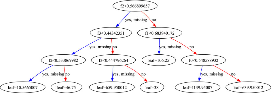
FIGURE 5. Visualization of decision tree prediction process.

To further compare the performance differences of different SCE models, Table 5 lists the performance of the three models on the COCOMO81 dataset. As can be seen from the table, deep learning-based algorithms such as HACO-BA performed poorly, mainly due to insufficient training data sets resulting in underfitting of the model. Compared to other algorithms, the model proposed in this article has a lower MdMRE value and a higher PRED value, indicating that the model has good consistency in prediction results across different project data, stable model performance, and high prediction accuracy. The cost evaluation in practical software engineering is mainly aimed at reducing development risks and promoting the rational allocation of resources, so the robustness of the prediction model is even more important. Comprehensively evaluated by various indicators, the model proposed in this article based on Autoencoder and Random Forest has better performance.

TABLE 5

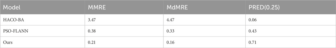
TABLE 5. Performance of different models on the COCOMO81 dataset.

In subsequent engineering analysis, factor analysis methods can be used to draw radar charts to further analyze the factors that affect the size of software cost, and rational allocation of resources can be used to make up for development shortcomings, thereby accelerating the software development process. We combine the scree plot method and practical significance of SCE to comprehensively determine the optimal number of factors. When the number of factors is 6, the eigenvalue of the matrix reaches the inflection point, and the expression rate of these factors reaches 81%. Therefore, the number of factors after dimensionality reduction is determined to be 6. By looking at the contribution rates of the original attributes to each factor, we named the six factors according to their practical significance. The radar chart of common factors after dimensionality reduction of a data sample is shown in Figure 6. It can be seen from the figure that the development environment of the project is relatively simple, and the R&D personnel have strong abilities. However, the software performance requirements and data scale are high, and the team’s collaboration ability is poor. Team managers should strengthen team communication and collaboration, and focus on algorithm design to reduce the spatial and temporal complexity of software, thereby achieving a multiplier effect.

FIGURE 6

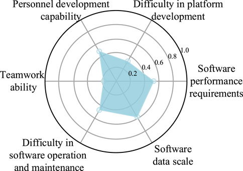
FIGURE 6. Radar chart of common factors for a project.

5 Conclusion

In order to adapt to the issue of comprehensive processing of social information and use it to improve production efficiency in CPSS, this paper proposes a novel SCE model based on Autoencoders and Random Forest, and evaluates its feasibility and performance through theoretical and experimental analysis. This article first introduces the improvement of Autoencoder and Random Forest algorithms on model accuracy and robustness, and analyzes the advantages of these two methods compared to traditional methods and neural network algorithms. Then, the overall framework and algorithm flow of the model are introduced, which are divided into four stages: data preprocessing, model training, cost prediction and result analysis. Finally, the performance of the model on three datasets, COCOMO81, Albrecht, and Desharnais, is introduced, and it is compared with common SCE algorithms to analyze the advantages and disadvantages of different algorithms. Compared with other algorithms, the proposed algorithm model has better accuracy and astringency, and can better complete the cost prediction task in practical software engineering.

At present, there is still much room for improvement in the evaluation models based on Autoencoder and Random Forest, such as low accuracy on datasets with ordinal attributes and significant influence by dataset on model accuracy. Future work should focus more on data processing and data imbalance issues to further improve the performance of the model.

Data availability statement

The original contributions presented in the study are included in the article/Supplementary Material, further inquiries can be directed to the corresponding author.

Author contributions

WZ: Conceptualization, Data curation, Formal Analysis, Investigation, Methodology, Software, Writing–original draft. HC: Funding acquisition, Resources, Supervision, Writing–review and editing. SZ: Data curation, Writing–review and editing. ML: Formal Analysis, Writing–review and editing. FW: Software, Writing–review and editing. ZH: Funding acquisition, Writing–review and editing.

Funding

The author(s) declare financial support was received for the research, authorship, and/or publication of this article. This study is supported by Sichuan Science and Technology Program (NO. 2022YFG0176), and Fundamental Research Funds for the Central Universities (No. ZYGX2021YGLH211).

Conflict of interest

Authors WZ, ML, FW and ZH were employed by PetroChina Southwest Oil and Gasfield Company.

The remaining authors declare that the research was conducted in the absence of any commercial or financial relationships that could be construed as a potential conflict of interest.

Publisher’s note

All claims expressed in this article are solely those of the authors and do not necessarily represent those of their affiliated organizations, or those of the publisher, the editors and the reviewers. Any product that may be evaluated in this article, or claim that may be made by its manufacturer, is not guaranteed or endorsed by the publisher.

Supplementary material

The Supplementary Material for this article can be found online at: https://www.frontiersin.org/articles/10.3389/fphy.2024.1324719/full#supplementary-material

References

1. Keung J. Software development cost estimation using analogy: a review. In: 2009 Australian Software Engineering Conference; 14-17 April 2009; Gold Cost, Australia (2009). doi:10.1109/ASWEC.2009.32

CrossRef Full Text | Google Scholar

2. Chirra SMR, Reza H. A survey on software cost estimation techniques. J Softw Eng Appl (2019) 12(06):226–48. doi:10.4236/jsea.2019.126014

CrossRef Full Text | Google Scholar

3. Saleem MA, Ahmad R, Alyas T, Idrees M, Farooq A Systematic literature review of identifying issues in software cost estimation techniques. Int J Adv Comp Sci Appl (2019) 10(8):10. doi:10.14569/ijacsa.2019.0100844

CrossRef Full Text | Google Scholar

4. Jorgensen M, Shepperd M. A systematic review of software development cost estimation studies. IEEE Trans Softw Eng (2007) 33(1):33–53. doi:10.1109/TSE.2007.256943

CrossRef Full Text | Google Scholar

5. Latif AM, Khan KM, Duc AN. Software cost estimation and capability maturity model in context of global software engineering. IGI Global (2022). 910–928. doi:10.4018/978-1-6684-3702-5.ch045

CrossRef Full Text | Google Scholar

6. Martinez-Fernandez S, Bogner J, Franch X, Oriol M, Siebert J, Trendowicz A, et al. Software engineering for ai-based systems: a survey. ACM Trans Softw Eng Methodol (2022) 31(2):1–59. doi:10.1145/3487043

CrossRef Full Text | Google Scholar

7. Tomasevic N, Gvozdenovic N, Vranes S. An overview and comparison of supervised data mining techniques for student exam performance prediction. Comput Edu (2020) 143:103676. doi:10.1016/j.compedu.2019.103676

CrossRef Full Text | Google Scholar

8. Esteve M, Aparicio J, Rabasa A, Rodriguez-Sala JJ. Efficiency analysis trees: a new methodology for estimating production Frontiers through decision trees. Expert Syst Appl (2020) 162:113783. doi:10.1016/j.eswa.2020.113783

CrossRef Full Text | Google Scholar

9. Elyassami S, Idri A. Applying fuzzy Id3 decision tree for software effort estimation (2011). Available at: https://arxiv.org/abs/1111.0158 (Accessed October 1, 2023).

Google Scholar

10. Asheeri MMA, Hammad M. Machine learning models for software cost estimation. In: 2019 International Conference on Innovation and Intelligence for Informatics, Computing, and Technologies (3ICT); 2019 22-23 September; Bahrain (2019). doi:10.1109/3ICT.2019.8910327

CrossRef Full Text | Google Scholar

11. abdelali Z, Mustapha H, Abdelwahed N. Investigating the use of random forest in software effort estimation. Proced Comp Sci (2019) 148:343–52. doi:10.1016/j.procs.2019.01.042

CrossRef Full Text | Google Scholar

12. Priya Varshini AG, Anitha Kumari K, Janani D, Soundariya S. Comparative analysis of machine learning and deep learning algorithms for software effort estimation. J Phys Conf Ser (2021) 1767(1):012019. doi:10.1088/1742-6596/1767/1/012019

CrossRef Full Text | Google Scholar

13. Grattarola D, Alippi C. Graph neural networks in tensorflow and keras with spektral [application notes]. IEEE Comput Intelligence Mag (2021) 16(1):99–106. doi:10.1109/mci.2020.3039072

CrossRef Full Text | Google Scholar

14. Prabha CL, Shivakumar N. Software defect prediction using machine learning techniques. In: 2020 4th International Conference on Trends in Electronics and Informatics (ICOEI)(48184); 15-17 June 2020; Tirunelveli, India (2020). doi:10.1109/ICOEI48184.2020.9142909

CrossRef Full Text | Google Scholar

15. Sharma D, Chandra P. Identification of latent variables using, factor analysis and multiple linear regression for software fault prediction. Int J Syst Assur Eng Manag (2019) 10(6):1453–73. doi:10.1007/s13198-019-00896-5

CrossRef Full Text | Google Scholar

16. Hamada MA, Abdallah A, Kasem M, Abokhalil M. Neural network estimation model to optimize timing and schedule of software projects. In: 2021 IEEE International Conference on Smart Information Systems and Technologies (SIST); 2021 28-30 April (2021). doi:10.1109/SIST50301.2021.9465887

CrossRef Full Text | Google Scholar

17. Heiat A. Comparison of artificial neural network and regression models for estimating software development effort. Inf Softw Tech (2002) 44(15):911–22. doi:10.1016/s0950-5849(02)00128-3

CrossRef Full Text | Google Scholar

18. Xie W, Liu B, Li Y, Lei J, Du Q. Autoencoder and adversarial-learning-based semisupervised background estimation for hyperspectral anomaly detection. IEEE Trans Geosci Remote Sensing (2020) 58(8):5416–27. doi:10.1109/tgrs.2020.2965995

CrossRef Full Text | Google Scholar

19. Yu W, Kim IIY, Mechefske C. Remaining useful life estimation using a bidirectional recurrent neural network based autoencoder scheme. Mech Syst Signal Process (2019) 129:764–80. doi:10.1016/j.ymssp.2019.05.005

CrossRef Full Text | Google Scholar

20. Chen T, Guestrin C. Xgboost: a scalable tree boosting system. In: Proceedings of the 22nd ACM SIGKDD International Conference on Knowledge Discovery and Data Mining; San Francisco, California, USA: Association for Computing Machinery; August 13 - 17, 2016; San Francisco, California, USA (2016). p. 785–94. doi:10.1145/2939672.2939785

CrossRef Full Text | Google Scholar

21. Musilek P, Pedrycz W, Nan S, Succi G. On the sensitivity of cocomo ii software cost estimation model. In: Proceedings Eighth IEEE Symposium on Software Metrics; 2002; 4-7 June 2002; Ottawa, Canada (2002). doi:10.1109/METRIC.2002.1011321

CrossRef Full Text | Google Scholar

22. Sahin CB. The role of vulnerable software metrics on software maintainability prediction. Avrupa Bilim ve Teknoloji Dergisi (2021)(23) 686–96. doi:10.31590/ejosat.858720

CrossRef Full Text | Google Scholar