An efficient approximate analytical technique for the fractional model describing the solid tumor invasion

In this manuscript, we derive and examine the analytical solution for the solid tumor invasion model of fractional order. The main aim of this work is to formulate a solid tumor invasion model using the Caputo fractional operator. Here, the model involves a system of four equations, which are solved using an approximate analytical method. We used the fixed-point theorem to describe the uniqueness and existence of the model’s system of solutions and graphs to explain the results we achieved using this approach. The technique used in this manuscript is more efficient for studying the behavior of this model, and the results are accurate and converge swiftly. The current study reveals that the investigated model is time-dependent, which can be explored using the fractional-order calculus concept.

1 Introduction

After the evolution of Homo sapiens (human beings), humans are still suffering from many diseases. Among those, cancer affects the population most significantly, ranking as the second most common cause of death after cardiovascular disease. Nearly 10 million deaths have occurred, according to a 2020 survey [1]. The first cancer tumor was discovered around 3000 BCE in Egyptian mummies. Malignant tumors and neoplasms are generally called cancer [2]. The process of scattering and creating secondary tumors is known as metastasis, and this behavior of cancer cells is the key reason for death in cancer patients. However, the cause of cancer was discovered by a British surgeon Percivall Pott in 1775. The estimation of the size, phase, and growth of a tumor is very critical for the treatment of cancer, and mathematics plays an important role in helping us investigate the behavior of the tumor. Many researchers have been studying the growth of solid tumors using mathematical models [3, 4]. Discrete models that consider single cells have been constructed on them. Jeon et al., invented the discrete-continuum model [5], which gives the idea of transporting chemicals inside the tumor and the individual character of cells. Solid tumors depend on diffusion because it is the only way to intake nutrients and detach waste products. One single normal cell is converted into a main solid tumor (e.g., carcinoma [6]) due to mutations in key genes. A single tumor cell has the potential to form a group of tumor cells through successive divisions, and they develop in two different stages: one is the vascular stage, and another is the avascular stage. Then, it will cause the formation of an avascular tumor with 10⁶ cells. Once solid tumors develop, they find a way to spread to other body parts through the circulatory system, leading to the destruction of normal tissues, and once a tumor reaches its maximum size, the absorption of nutrients is insufficient to provide the tumor’s inner parts with oxygen, which causes cell death. There are many experimental ways to model tumor cell migration, like macro-scale models and micro-patterned models [7, 8]. These solid tumors are formed due to the production of abnormal cells in the body. Another reason for the formation of solid tumors is the non-replication of DNA at the molecular level in the cell nucleus. As much research has been done and developed, many anti-cancer therapies, like radiation therapy, chemotherapy, and hormone therapy and surgery, have been implemented to increase lifespan and reduce tumors. These traditional cancer treatments do not cure it completely but involve other side effects like fatigue, vomiting, hair loss, and a reduction in blood count. However, there is a therapy called virotherapy [9], where several viruses have been used as agents to treat cancer cells, and clinical trials proved zero percent toxicity. In recent years, many mathematical models of solid tumor growth [10–13] have been established, and they have also concentrated on the evolutionary dynamics of tumor growth. In this article, we will examine the solid tumor invasion model [14] of fractional order, and this model is expressed as a system of partial differential equations. The interactions between the cancer cells are denoted by $T_d$, matrix-degrading enzymes (MDEs) are represented by $M_c$, the extracellular matrix is signified by $E_c$, and the rate of oxygen production is given by $O_c$. Regarding the extracellular matrix, the majority of the macromolecules are necessary for adhesion, spreading, and motility of cells. Moreover, several macromolecules, including collagen, laminin, and fibronectin, are linked to the extracellular matrix. Matrix-degrading enzymes are essential for different phases of invasion, metastasis, and turnover growth. Tumor cells produce matrix-degrading enzymes that cause the extracellular matrix to break down locally. Additionally, the way they interact with growth factors, inhibitors, and tumor cells is very complex. Here, $T_d$ and $M_c$ and $E_c$ and $O_c$ have a direct linear relationship.

Fractional calculus (FC) is a tool to study derivatives and integrals of fractional order. As we know, classical calculus has been developed as a vast subject, and many researchers have been working on it until now. Due to the ideas of German mathematician Leibniz and L’Hospital’s rule, the theory of fractional calculus came into existence approximately 300 years ago. Fractional calculus can be assumed to be a well-developed and established subject. Both memory effects and hereditary properties influence the problem under consideration. FC has attracted many researchers to work on it. Compared to classical calculus, fractional calculus has more applications in various fields and real-world problems, as it gives solutions in between the intervals [15]. We all know that classical differential equations have numerous applications that model many natural and physical phenomena, but fractional differential equations (FDEs) model natural and physical phenomena more accurately, as the behaviors of FDEs give an accurate and approximate solution to the problem, which can be analyzed more understandably. Fractional-order derivatives have a greater ability to model complicated non-linear processes [16–19] and higher-order behaviors. The main reason to consider fractional derivatives is that we can take any order of derivative rather than restricting it to integer order. FC has a wide variety of applications in the fields of science [20], biology [21, 22], engineering [23], and others. It allows us to study many physical phenomena, like earthquake vibrations, elasticity, shallow water waves, and quantum mechanics [24–27]. Many researchers have defined fractional derivatives like Riemann–Liouville, Caputo derivative, Grünwald–Letnikov, and Atangana–Baleanu, but each operator has its own limitations. The linear and non-linear FDEs can be solved using the variational iteration method [28, 29], differential transform method [30, 31], q-homotopy analysis transform method [32], residual power series method [33], homotopy perturbation method [34, 35], and many analytical, numerical, and other techniques [36–41, 57] which give analytical, numerical, and exact solutions. Recently, [42] investigated giving up smoking models with non-singular derivatives. [43] proposed the cancer-immune system model of fractional order using Caputo and Caputo–Fabrizio derivatives. [44] demonstrated the behavior of the cancer cells after injecting a dose of medicine by developing a new cancer model. [45] developed a new cancer mathematical model of fractional order using IL-10 cytokine and anti-PD-L1 inhibitors. [46–48] implemented the similarity method to study multi-term time-fractional diffusion equations, Riesz fractional partial differential equations, and fractional heat equations and also deduced two variable fractional partial differential equations from ordinary differential equations. Many biological, epidemical, and other mathematical models have been studied [49–56]. Here, we will apply an efficient technique called the approximate analytical method (AAM) to study the considered model. AAM is a semi-analytical method that can be used to solve highly non-linear problems, as it gives a series solution, allowing us to analyze the solution more effectively. The significance of this method is that it discretizes the non-linear terms in the equations. AAM can be applied to solve complex non-linear and linear fractional differential equations and requires less computational work. AAM has been applied to solve solute problems, fluid flow models, and KDV equations [57, 58].

2 Preliminaries

The following definitions and properties, which are utilized in this article, are cited in [17, 18, 50].

Definition 2.1: The fractional integral of a function $f\left(t\right)\in C_{\mu }\left(\mu \ge -1\right)$ of non-zero positive order $\alpha$ is defined by Riemann–Liouville (RL) and represented by

${}_0{J}_t^{\alpha }f\left(t\right)=\frac{1}{\mathrm{\Gamma }\left(\alpha \right)}{\int }_0^t{\left(t-\vartheta \right)}^{\alpha -1}f\left(\vartheta \right)d\vartheta ,J^{0}f\left(t\right)=f\left(t\right).$

Theorem 2.2: Let $b>-1$ and ${\alpha }_1,{\alpha }_2\mathbb{\in }\mathbb{R},{\alpha }_1,{\alpha }_2\ge 0$. Then, the RL fractional partial integral operator ${}_0{J}_t^{\alpha }$ satisfies the following properties for the function $u\left(x,t\right)\in C_{\mu ,}\mu >-1$:

${}_0{J}_t^{{\alpha }_1}{}_0{J}_t^{{\alpha }_2}u\left(x,y,t\right)={}_0{J}_t^{{\alpha }_1+{\alpha }_2}u\left(x,y,t\right),{}_0{J}_t^{{\alpha }_1}{}_0{J}_t^{{\alpha }_2}u\left(x,y,t\right)={}_0{J}_t^{{\alpha }_2}{}_0{J}_t^{{\alpha }_1}u\left(x,y,t\right),{}_0{J}_t^{\alpha }{t}^b=\frac{\mathrm{\Gamma }\left(b+1\right)}{\mathrm{\Gamma }\left(b+\alpha +1\right)}{t}^{\alpha +b}.$

Definition 2.3. The fractional derivative of $f\in C_{-1}^n$ in the Caputo sense is defined as

$D_t^{\alpha }f\left(t\right)=\left\{\begin{array}{l}\frac{d^{n}f\left(t\right)}{d{t}^n},\alpha =n\mathbb{\in }\mathbb{N},\\ \frac{1}{\mathrm{\Gamma }\left(n-\alpha \right)}{\int }_0^t{\left(t-\vartheta \right)}^{n-\alpha -1}{f}^{\left(n\right)}\left(\vartheta \right)d\vartheta ,\alpha \in \left(n-1,n\right),n\mathbb{\in }\mathbb{N}.\end{array}\right.$

Definition 2.4. The Laplace transform (LT) of a Caputo fractional derivative $D_t^{\alpha }f\left(t\right)$ is denoted as

$L\left[D_t^{\alpha }f\left(t\right)\right]=s^{\alpha }F\left(s\right)-{\displaystyle {\sum }_{r=0}^{n-1}}{s}^{\alpha -r-1}{f}^{\left(r\right)}\left(0^{+}\right),\left(n-1<\alpha \le n\right),$

where $F\left(s\right)$ denotes the LT of the function f(t).

Theorem 2.5: Let $\alpha ,t\mathbb{\in }\mathbb{R},t\ge 0,n-1<\alpha <n\mathbb{\in }\mathbb{N}$. Then, we have

$D_t^{\alpha }{}_0{J}_t^{\alpha }u\left(x,y,t\right)=u\left(x,y,t\right),{}_0{J}_t^{\alpha }{}_0{D}_t^{\alpha }u\left(x,y,t\right)=u\left(x,y,t\right)-{\sum }_{k=0}^{m-1}\frac{t^k}{k!}\frac{{\partial }^{k}u\left(x,y,0^{+}\right)}{{\partial t}^k}.$

3 Mathematical model of solid tumor invasion

3.1 Classical model

Let us consider the classical model of solid tumor invasion, which involves a system of partial differential equations: $M_c$ indicates the matrix-degrading enzyme (MDE) concentration, $T_d$ indicates the tumor cell density, $O_c$ indicates the oxygen concentration, $E_c$ indicates the concentration of macromolecules (MMs) in the extracellular matrix (EC). The values of all four variables depend on both x and time ζ. The motion of the tumor cells is determined by [14]

$\frac{\partial T_d}{\partial \zeta }=d_n{\nabla }^2{T}_d-\rho \nabla \left(T_d\nabla E_c\right).$

The value of the arbitrary motility coefficient that remains constant is denoted by $d_n$, while the haptotatic coefficient is represented by ρ > 0. The breakdown of the ECM occurs due to MDEs). This leads to a process of deterioration, which is given by

$\frac{\partial E_c}{\partial \mathrm{\zeta }}=-\delta {M_{c}E}_c,$

where $\delta$ is a positive constant. It is believed that active MDEs are generated by tumor cells, dispersed throughout the tissue, and undergo a certain level of decomposition. The definition for the concentration of MDE is as follows:

$\frac{\partial M_c}{\partial \zeta }=d_m{\nabla }^2{M}_c+\mu T_d-\lambda M_c,$

where the positive constants are represented as $\lambda$, $d_m,\text{and\hspace{0.17em}}\mu$. The diffusion coefficient of MDEs is denoted by $d_m$.

Solid tumor needs oxygen for growth and invasion. Oxygen gets distributed among the macromolecules, undergoes decay, and is eventually absorbed by the tumor. The density of MM is directly related to the manufacture of oxygen. It is specified by

$\frac{\partial O_c}{\partial \zeta }=d_c{\nabla }^2{O}_c+\beta E_c-\gamma M_c-\mathrm{\alpha }{O}_c,$

where the rate of production is given by $\beta$, the diffusion coefficient of oxygen is denoted by $d_{\begin{array}{c}c\end{array}}$, the rate of decay is given by $\alpha$, the rate of uptake is given by $\gamma$, and all other variables remain constant.

The system of equations is given by

$\frac{\partial T_d}{\partial \zeta }=d_n{\nabla }^2{T}_d-\rho \nabla \left(T_d\nabla E_c\right),\frac{\partial E_c}{\partial \mathrm{\zeta }}=-\delta {M_{c}E}_c,\frac{\partial M_c}{\partial \zeta }=d_m{\nabla }^2{M}_c+\mu T_d-\lambda M_c,\frac{\partial O_c}{\partial \zeta }=d_c{\nabla }^2{O}_c+\beta E_c-\gamma M_c-\mathrm{\alpha }{O}_c.$

The adhesion between cells and the extracellular matrix is framed by the outgrowth of cells in the cell equation, represented by χ. The system is designed to operate within a square spatial domain Ω, which represents tissue. It includes specific initial conditions for every variable. It is believed that the variables stay within the tissue area under consideration. As a result, boundary ∂Ω is subjected to no-flux boundary conditions.

We can achieve dimensionless equations by implementing non-dimensionalization through appropriate parameters such as length scale L and time $\tau$. This approach helps simplify the equations and makes them easier to analyze; we scale the parameters as follows: the density of the tumor cell as $T_{d0}$, the density of the ECM as $E_{c0}$, the concentration of the MDE as $M_{c0}$, and the concentration of oxygen as $O_{c0}$.

$\stackrel{\sim }{T_d}=\frac{T_d}{T_{d0}},\stackrel{\sim }{E_c}=\frac{E_c}{E_{c0}},\stackrel{\sim }{M_c}=\frac{M_c}{M_{c0}},\stackrel{\sim }{O_c}=\frac{O_c}{O_{c0}},\stackrel{\sim }{x}=\frac{x}{L},\stackrel{\sim }{\mathrm{\zeta }}=\frac{\mathrm{\zeta }}{L}.$

Now, the equations are given by

$\frac{\partial T_d}{\partial \zeta }=D_n{\nabla }^2{T}_d-\chi \nabla \left(T_d\nabla E_c\right),\frac{\partial E_c}{\partial \mathrm{\zeta }}=-{{\mathrm{\eta }M}_{c}E}_c,\frac{\partial M_c}{\partial \zeta }=D_m{\nabla }^2{M}_c+k{T}_d-\sigma M_c,\frac{\partial O_c}{\partial \zeta }=D_c{\nabla }^2{O}_c+\gamma E_c-\omega M_c-\varphi O_c.(1)$

where $D_m$ = $\frac{\tau d_n}{L^2}$, $D_n$ = $\frac{d_m\tau }{L^2}$, $D_{\begin{array}{c}c\end{array}}=\frac{\tau d_c}{L^2}$, ꭓ = $\frac{\tau E_{c0}}{L^2}$, $\mathrm{\eta }=\tau M_{c0}\delta$, k = $\frac{\tau \mu T_{d0}}{M_{c0}}$, $\sigma =\tau \mathrm{\lambda }$, $\gamma =\frac{\tau \beta E_{c0}}{O_{c0}}$, $\omega =\frac{\tau \gamma T_{d0}}{O_{c0}}$, and $ɸ=\tau \alpha$.

3.2 Fractional model

By using the Caputo fractional derivative, the system of equations (Eq. 1) has been converted into fractional differential equations.

${}_{t_0}{}^c{D}_{\zeta }^{\alpha }{T}_d=D_n{\nabla }^2{T}_d-\chi \nabla \left(T_d\nabla E_c\right),{}_{t_0}{}^c{D}_{\zeta }^{\alpha }{E}_c=-{{\mathrm{\eta }M}_{c}E}_c,{}_{t_0}{}^c{D}_{\zeta }^{\alpha }{M}_c=D_m{\nabla }^2{M}_c+k{T}_d-\sigma M_c,{}_{t_0}{}^c{D}_{\zeta }^{\alpha }{O}_c=D_c{\nabla }^2{O}_c+\gamma E_c-\omega M_c-\varphi O_c,(2)$

with the initial conditions

$T_{d_0}=T_d\left(x,0\right)=e^{\frac{{-x}^2}{\epsilon }},E_{c_0}=E_c\left(x,0\right)=1-0.5e^{\frac{{-x}^2}{\epsilon }},M_{c_0}=M_c\left(x,0\right)=0.5e^{\frac{{-x}^2}{\epsilon }},O_{c_0}=O_c\left(x,0\right)=0.5e^{\frac{{-x}^2}{\epsilon }}.$

4 Methodology of the approximate analytical method

In order to determine the validity of this approach, we will examine the non-linear fractional partial differential equation (NFPDE) with the following initial conditions:

$D_t^{\alpha }u\left(\overline{x},\overline{y},t\right)=f\left(\overline{x},\overline{y},t\right)+L\overline{u}+N\overline{u},m-1<\alpha <m\in N,\frac{{\partial }^{i}u\left(\overline{x},\overline{y},t\right)}{\partial t^i}=f_i\left(\overline{x},\overline{y}\right),i=0,1,2,3,\dots .m-1,(3)$

where $D_t^{\alpha }$ is the Caputo fractional partial derivative of order $\alpha ,f\left(\overline{x},\overline{y},t\right)$ is the source term, which is an analytical function, L and N represent linear and non-linear operators, and $\overline{x}=\left(x_1,x_2,\dots ,x_n\right)$ $\overline{y}=\left(y_1,y_2,\dots ,y_n\right)\in {\mathbb{R}}^n$. To attain the analytical solution of the considered model, we implemented a technique called the approximate analytical method. Computational accuracy is necessary to provide appropriate piecewise analytical solutions, making it a useful tool for solving non-linear fractional differential equations. To illustrate AAM, it is essential to analyze the subsequent outcomes. The outcomes are cited in [48, 50].

Lemma 4.1: For $v\left(\overline{x},\overline{y},t\right)={\displaystyle {\sum }_{k=0}^{\infty }}{r}^{k}v\left(\overline{x},\overline{y},t\right),$ the linear operator $L\left(u\right)$ satisfies the following property:

$L\left(v\left(\overline{x},\overline{y},t\right)\right)=L\left({\displaystyle \sum _{k=0}^{\infty }}{r}^{k}v\left(\overline{x},\overline{y},t\right)\right)={\displaystyle \sum _{k=0}^{\infty }}{r}^{k}L{v}_k\left(\overline{x},\overline{y},t\right).$

Theorem 4.2. Let $v\left(\overline{x},\overline{y},t\right)={\displaystyle {\sum }_{k=0}^{\infty }}{v}_k\left(\overline{x},\overline{y},t\right)$ and $v_{\lambda }\left(\overline{x},\overline{y},t\right)={\displaystyle {\sum }_{k=0}^{\infty }}{\lambda }^k{v}_k\left(\overline{x},\overline{y},t\right)$, where λ is the non-zero parameter such that $0\le \lambda \le 1$, and subsequently, the non-linear operator $N\left(v_{\lambda }\right)$ satisfies the following conditions:

$N\left(v_{\lambda }\right)=N{\displaystyle {\sum }_{k=0}^{\infty }}\left({\lambda }^k{v}_k\right)={\displaystyle {\sum }_{n=0}^{\infty }}\left(\frac{1}{n!}\frac{\delta }{\delta {\lambda }^n}{\left(N\left({\displaystyle {\sum }_{k=0}^{\infty }}{\lambda }^k{v}_k\right)\right)}_{\lambda =0}\right){\lambda }^n.$

Proof: Consider the Maclaurin expansion concerning 𝜆λ, which gives

$\begin{array}{l}N\left(v_{\lambda }\right)=N\left({\sum }_{k=0}^{\infty }{\lambda }^k{v}_k\right)={\left[N{\sum }_{k=0}^{\infty }\left({\lambda }^k{v}_k\right)\right]}_{\lambda =0}+\left[\frac{\delta }{\delta \lambda }\left[{\left[N{\sum }_{k=0}^{\infty }\left({\lambda }^k{v}_k\right)\right]}_{\lambda =0}\right]\right]\lambda +\left[\frac{1}{2!}\frac{{\delta }^2}{{\delta \lambda }^2}\left[{\left[N{\sum }_{k=0}^{\infty }\left({\lambda }^k{v}_k\right)\right]}_{\lambda =0}\right]\right]{\lambda }^2+\dots =\\ {\sum }_{k=0}^{\infty }\left(\frac{1}{n!}\frac{{\delta }^n}{{\delta \lambda }^n}{\left(N\left({\sum }_{k=0}^{\infty }{\lambda }^k{v}_k\right)\right)}_{\lambda =0}\right){\lambda }^n={\sum }_{k=0}^{\infty }\left(\frac{1}{n!}\frac{{\delta }^n}{{\delta \lambda }^n}{\left(N\left({\sum }_{k=0}^{\infty }{\lambda }^k{v}_k+{\sum }_{k=n+1}^{\infty }{\lambda }^k{v}_k\right)\right)}_{\lambda =0}\right){\lambda }^n={\sum }_{k=0}^{\infty }\left(\frac{1}{n!}\frac{{\delta }^n}{{\delta \lambda }^n}{\left(N\left({\sum }_{k=0}^{\mathrm{n}}{\lambda }^k{v}_k\right)\right)}_{\lambda =0}\right){\lambda }^n.\end{array}$

Definition 4.3: The polynomials $P_n\left(v_0,v_1,v_2,\dots v_n\right)$ are defined as follows:

$P_n\left(v_0,v_1,v_2,\dots v_n\right)=\frac{1}{n!}\frac{{\delta }^n}{{\delta \lambda }^n}{\left(N\left({\sum }_{k=0}^{\mathrm{n}}{\lambda }^k{v}_k\right)\right)}_{\lambda =0}.$

Remark 4.4. Let $P_n=P_n\left(v_0,v_1,v_2,\dots v_n\right)$, as shown in Definition 4.3. The non-linear term $N\left(v_{\lambda }\right)$ can be defined in terms of $P_n$ using Theorem 4.2 as follows:

$N\left(v_{\lambda }\right)={\displaystyle {\sum }_{n=0}^{\infty }}{\lambda }^n{P}_n.$

4.1 Existence theorem

The following theorem presents an approximate analytical solution for a non-linear fractional partial differential equation, with its initial solution given in Eq. 3 and obtained through the AAM.

Theorem 4.6: The functions $f\left(\overline{x},t\right)\text{\hspace{0.17em}and\hspace{0.17em}}{f}_i\left(\overline{x}\right)$ are defined as shown in Eq. 3 and $m-1<\mathrm{\alpha }<m\mathbb{\in }\mathbb{N}$.

Equation 3 gives at least one solution, which is provided by

$v\left(\overline{x},\overline{y},t\right)=f_t^{\left(-\alpha \right)}\left(\overline{x},\overline{y},t\right)+{\displaystyle {\sum }_{i=0}^{m-1}}\frac{t^i}{i!}{f}_i\left(\overline{x},\overline{y}\right)+{\displaystyle {\sum }_{i=0}^{m-1}}\left[L_t^{-\alpha }{v}_{\left(k-1\right)}+p_{\left(k-1\right)t}^{\left(-\alpha \right)}\right],$

where $p_{\left(k-1\right)t}^{\left(-\alpha \right)}$ and $L_t^{-\alpha }{v}_{\left(k-1\right)}$ are the Riemann–Liouville partial fractional integral of order $\alpha$ for $P_{k-1}$ and $L\left(v_{k-1}\right)$ with regard to t, respectively.

Proof: Consider the solution $v\left(\overline{x},\overline{y},t\right)$ of Eq. 3 in the analytical form:

$v\left(\overline{x},\overline{y},t\right)={\sum }_{k=0}^{\infty }{v}_k\left(\overline{x},\overline{y},t\right).(4)$

Let us consider the below expression to solve the given initial value problem shown in Eq. 3:

$D_t^{\alpha }{v}_{\lambda }\left(\overline{x},\overline{y},t\right)=\lambda \left[f\left(\overline{x},\overline{y},t\right)+L\left(v_{\lambda }\right)+N\left(v_{\lambda }\right)\right],0\le \lambda \le 1,(5)$

with initial conditions

$\frac{{\partial }^{i}u\left(\overline{x},\overline{y},t\right)}{\partial t^i}=f_i\left(\overline{x},\overline{y}\right),i=0,1,2,3,\dots .m-1.(6)$

Let us suppose that Eq. 5 has the solution in the form:

$v_{\lambda }\left(\overline{x},\overline{y},t\right)={\sum }_{k=0}^{\infty }{{\lambda }^{k}v}_k\left(\overline{x},\overline{y},t\right).(7)$

Now, let us consider Eq. 3 with the Riemann–Liouville partial integral, and using Theorem 4.2, we have

$v_{\lambda }\left(\overline{x},\overline{y},t\right)={\sum }_{i=0}^{m-1}\frac{t^i}{i!}\frac{{\partial }^i{v}_{\lambda }\left(\overline{x},\overline{y},0\right)}{\partial t^i}+\lambda {}_0{J}_t^{\alpha }\left[f(\left(\overline{x},\overline{y},t\right)+L\left(v_{\lambda }\right)+N\left(v_{\lambda }\right)\right].(8)$

Equation 8 can be written as below using Eq. 6:

$v_{\lambda \left(\overline{x},\overline{y},t\right)}={\sum }_{i=0}^{m-1}\frac{t^i}{i!}{g}_i\left(\overline{x},\overline{y}\right)+\lambda \left[f_t^{\left(-\alpha \right)}\left(\overline{x},\overline{y},t\right)+J_t^{\alpha }\left[L\left(v_{\lambda }\right)\right]+J_t^{\alpha }\left[N\left(v_{\lambda }\right)\right]\right].(9)$

By substituting Eq. 7 into Eq. 9, we obtain

${\sum }_{k=0}^{\infty }{\lambda }^k{v}_k\left(\overline{x},\overline{y},t\right)={\sum }_{i=0}^{m-1}\frac{t^i}{i!}{g}_i\left(\overline{x},\overline{y}\right)+\lambda f_t^{\left(-\alpha \right)}\left(\overline{x},\overline{y},t\right)+J_t^{\alpha }\lambda {\sum }_{k=0}^{\infty }\left[L\left({\lambda }^k{v}_k\right)\right]+J_t^{\alpha }\lambda {\sum }_{n=0}^{\infty }\left[\frac{1}{n!}\frac{{\partial }^n}{{\partial \lambda }^n}{\left(N\left({\sum }_{k=0}^{\infty }{\lambda }^k{v}_k\right)\right)}_{\lambda =0}\right]{\lambda }^n.(10)$

With the help of definition 4.3 and Eq. 10, we obtain

${\sum }_{k=0}^{\infty }{\lambda }^k{v}_k\left(\overline{x},\overline{y},t\right)={\sum }_{i=0}^{m-1}\frac{t^i}{i!}{g}_i\left(\overline{x},\overline{y}\right)+\lambda f_t^{\left(-\alpha \right)}\left(\overline{x},\overline{y},t\right)+J_t^{\alpha }\lambda {\sum }_{k=0}^{\infty }\left[L\left({\lambda }^k{v}_k\right)\right]+J_t^{\alpha }\lambda {\sum }_{n=0}^{\infty }{p}_n{\lambda }^n.(11)$

Equating the coefficients of like powers of $\mathrm{\lambda }$ in Eq. 11, we get the below terms

$v_o{\sum }_{i=0}^{m-1}\frac{t^i}{i!}{g}_i\left(\overline{x},\overline{y}\right),v_1\left(\overline{x},\overline{y},t\right)=f_t^{\left(-\alpha \right)}\left(\overline{x},\overline{y},t\right)+L_t^{\left(-\alpha \right)}{v}_0+P_{ot}^{\left(-\alpha \right)},v_1\left(\overline{x},\overline{y},t\right)=L_t^{\left(-\alpha \right)}{v}_{k-1}+P_{\left(k-1\right)t}^{\left(-\alpha \right)},k=2,3,(12)$

Substituting Eq. 12 into Eq. 7 gives the solution of Eq. 3. Using Eq. 4 and 7, we obtain

$v\left(\overline{x},\overline{y},t\right)=\underset{\lambda \to 1}{\lim }{v}_{\lambda }\left(\overline{x},\overline{y},t\right)=v_0\left(\overline{x},\overline{y},t\right)+v_1\left(\overline{x},\overline{y},t\right)+{\sum }_{k=2}^{\infty }{v}_k\left(\overline{x},\overline{y},t\right).(13)$

We can see that $\frac{{\partial }^{i}v\left(\overline{x},\overline{y},0\right)}{{\partial t}^i}=\underset{\lambda \to 1}{\lim }\frac{{{\partial }^{i}v}_{\lambda }\left(\overline{x},\overline{y},t\right)}{{\partial t}^i}\Rightarrow g_i\left(\overline{x},\overline{y}\right)=f_i\left(\overline{x},\overline{y}\right)$. Replacing Eq. 12 in Eq. 13 ends the proof.

5 Existence of the solution

We will explain the solution’s existence using the concepts provided below.

Definition 5.1: Let us consider a Cauchy space $\left(X,d\right)$, which is non-empty and $0\le \lambda <1$. If the mapping $S:X\to X$ for every $\left(x,\overline{x}\right)\in X$, then it satisfies

$d\left(Sx,S\overline{x}\right)\le \lambda d\left(x,\overline{x}\right).$

Then, S has a unique fixed point $x^{*}\in X$. If $S^k\left(k\in N\right)$, the sequence is given by

$\left\{\begin{array}{l}{S}^k=S{S}^{k-1,}k\mathbb{\in }\mathbb{N}/\left\{1\right\}\\ S^1=S\end{array}\right..$

Thus, for any $x_0\in X{,\left\{S_{x_0}^k\right\}}_{k=1}^{k=\infty }$ reaches the fixed point $x^{*}$.

Definition 5.2: Let $m\mathbb{\in }\mathbb{N}$, $H\in {\mathbb{R}}^m$, $\left[\mathrm{p},\mathrm{q}\right]\mathbb{\subset }\mathbb{R}$, and $h:\left[p,q\right]\times H\to \mathbb{R}$ be the function of $s,t$ for $\left(x_{1,}{x}_{2,}\dots ,x_m\right)\left({x_1}^{*},{x_2}^{*},\dots ,x_m^{*}\right)\in H$. Here, h satisfies the generalized Lipschitz condition: $\left|h\left(\zeta ,x_{1,}{x}_{2,}\dots ,x_m\right)-h\left(\zeta ,{x_1}^{*},{x_2}^{*},\dots {,x}_m^{*}\right)\right|\le A_1\left|x_1-{x_1}^{*}\right|+A_2\left|x_{2.}-{x_2}^{*}\right|+\dots +A_m\left|x_m-{x_m}^{*}\right|,A_j\ge 0,j=1,2,3\dots ,m$.

Specifically, h satisfies the Lipschitz condition. If $\forall ,\zeta \in (\left.p,q\right]$ and for any $x,x^{*}\in G,$ one has

$\left|h\left[\zeta ,x\right]-h\left[\zeta ,x^{*}\right]\right|\le A\left|x-x^{*}\right|,A>0.$

Let us examine the following set of equations:

$D_{\zeta }^{\alpha }\left[T_d\left(x,\zeta \right)\right]={\psi }_1\left(x,\zeta ,T_d\right),D_{\zeta }^{\alpha }\left[E_c\left(x,\zeta \right)\right]={\psi }_2\left(x,\zeta ,E_c\right),D_{\zeta }^{\alpha }\left[M_c\left(x,\zeta \right)\right]={\psi }_3\left(x,\zeta ,M_c\right),D_{\zeta }^{\alpha }\left[O_c\left(x,\zeta \right)\right]={\psi }_4\left(x,\zeta ,O_c\right).(14)$

Now using the above Eq. 14, we obtain

$T_d\left(x,\zeta \right)-T_d\left(x,0\right)=I_{\zeta }^{\alpha }\left\{D_n\frac{{\partial }^2}{{\partial x}^2}{T}_d-\chi \left(\frac{\partial T_d}{\partial x}\frac{\partial E_c}{\partial x}+T_d\frac{{\partial }^2{E}_c}{{\partial x}^2}\right)\right\},$

$E_c\left(x,\zeta \right)-E_c\left(x,0\right)=I_{\zeta }^{\alpha }\left\{-\eta M_c{E}_c\right\},$

$M_c\left(x,\zeta \right)-M_c\left(x,0\right)=I_{\zeta }^{\alpha }\left\{D_p\frac{{\partial }^2{M}_c}{{\partial x}^2}+k{T}_d-\sigma M_c\right\},$

$O_c\left(x,\zeta \right)-O_c\left(x,0\right)=I_{\zeta }^{\alpha }\left\{D_c\frac{{\partial }^2{O}_c}{{\partial x}^2}+\gamma E_c-\omega M_c-\varphi O_c\right\}.$

Then, by defining the fractional integral, we obtain

$\begin{array}{l}{T}_d\left(x,\zeta \right)-T_d\left(x,0\right)=\frac{1}{\mathrm{\Gamma }\left(\alpha \right)}{\int }_0^{\zeta }{\left(\zeta -v\right)}^{\alpha -1}{\psi }_1\left(x,v,T_d\right)dv,E_c\left(x,\zeta \right)-E_c\left(x,0\right)=\frac{1}{\mathrm{\Gamma }\left(\alpha \right)}{\int }_0^{\zeta }{\left(\zeta -v\right)}^{\alpha -1}{\psi }_2\left(x,v,E_c\right)dv,M_c\left(x,\zeta \right)-M_c\left(x,0\right)\\ =\frac{1}{\mathrm{\Gamma }\left(\alpha \right)}{\int }_0^{\zeta }{\left(\zeta -v\right)}^{\alpha -1}{\psi }_3\left(x,v,M_c\right)dv,O_c\left(x,\zeta \right)-O_c\left(x,0\right)=\frac{1}{\mathrm{\Gamma }\left(\alpha \right)}{\int }_0^{\zeta }{\left(\zeta -v\right)}^{\alpha -1}{\psi }_4\left(x,v,O_c\right)dv.\end{array}$

5.1 Convergence theorem

Let us consider a mapping $H:G\to G$, which is non-linear, with Banach space G. Let us suppose that

$‖H\left(u\right)-H\left(v\right)‖\le {\mu }_i‖u-v‖,\forall u,v\in G.$

Thus, it has a fixed point convergence to a singular point within H and

$‖v_m-v_p‖\le \frac{{\mu }_i^p}{1-{\mu }_i}‖v_1-v_0‖,i=1,2,3,4.$

Proof: Consider the Banach space $\left(C\left[J\right],‖.‖\right)$ with the norm demarcated as

$‖g\left(t\right)‖={\max }_{t\in J}\left|g\left(t\right)\right|\text{\hspace{0.17em}function\hspace{0.17em}on\hspace{0.17em}}J.$

We need to confirm whether the sequences $\left\{T_{d_p}\right\}$, $\left\{E_{c_p}\right\}$, and $\left\{O_{c_p}\right\}$ are Cauchy sequences in $\left(C\left[J\right],‖.‖\right)$.

For $T_{d_p}$, consider

$\begin{array}{l}‖T_{d_m}-T_{d_p}‖={\max }_{t\in J}\left|T_{d_m}-T_{d_p}\right|,\\ ={\max }_{t\in J}\left|\left(T_{d_{m-1}}-T_{d_{p-1}}\right)-{}_0{J}_t^{\alpha }\left(\left(D_n\frac{{\partial }^2{T}_{d_{m-1}}}{\partial x^2}-\frac{{\partial }^2{T}_{d_{p-1}}}{\partial x^2}\right)-x\left(\frac{{\partial \varsigma }_{d_{m-1}}}{\partial x}\frac{{\partial E}_{c_{m-1}}}{\partial x}+T_{d_{m-1}}\frac{{\partial }^2{E}_{c_{m-1}}}{\partial x^2}-\frac{{\partial \varsigma }_{d_{p-1}}}{\partial x}\frac{{\partial E}_{c_{p-1}}}{\partial x}-T_{d_{p-1}}\frac{{\partial }^2{E}_{c_{p-1}}}{\partial x^2}\right)\right)\right|\\ \le {\max }_{t\in J}\left|\left(T_{d_{m-1}}-T_{d_{p-1}}\right)-{}_0{J}_t^{\alpha }\left(\left(D_n\frac{{\partial }^2{T}_{d_{m-1}}}{\partial x^2}-\frac{{\partial }^2{T}_{d_{p-1}}}{\partial x^2}\right)-x\left(\frac{{\partial \varsigma }_{d_{m-1}}}{\partial x}\frac{{\partial E}_{c_{m-1}}}{\partial x}+T_{d_{m-1}}\frac{{\partial }^2{E}_{c_{m-1}}}{\partial x^2}-\frac{{\partial \varsigma }_{d_{p-1}}}{\partial x}\frac{{\partial E}_{c_{p-1}}}{\partial x}-T_{d_{p-1}}\frac{{\partial }^2{E}_{c_{p-1}}}{\partial x^2}\right)\right)\frac{{\left(\varsigma -v\right)}^{\alpha }}{\mathrm{\Gamma }\left(1+\alpha \right)}dv\right|\end{array}$

(by convolution theorem)

$\le \left|\left(T_{d_{m-1}}-T_{d_{p-1}}\right)\right|-{\int }_0^{\varsigma }{D}_n{\delta }_1^2+\chi \left({\delta }_1{\lambda }_1+{\lambda }_2\right)\frac{{\left(\varsigma -v\right)}^{\alpha }}{\mathrm{\Gamma }\left(1+\alpha \right)}\left|T_{d_{m-1}}-\right|dv,$

and the above inequality reduced to

$‖T_{d_m}-T_{d_p}‖\le {\mu }_1‖T_{d_{m-1}}-T_{d_{p-1}}‖,$

where

${\mu }_1={\int }_0^{\varsigma }{D}_n{\delta }_1^2+\chi \left({\delta }_1{\lambda }_1+{\lambda }_2\right)\frac{{\left(\varsigma -v\right)}^{\alpha }}{\mathrm{\Gamma }\left(1+\alpha \right)}dv,$

${\delta }_1=\frac{{\partial \varsigma }_{d_{m-1}}}{\partial x}-\frac{{\partial \varsigma }_{d_{p-1}}}{\partial x},{\delta }_2=\frac{{{\partial }^{2}T}_{d_{m-1}}}{\partial x^2}-\frac{{{\partial }^{2}T}_{d_{p-1}}}{\partial x^2},$

${\lambda }_1=\frac{{\partial E}_{c_{m-1}}}{\partial x}-\frac{{\partial E}_{c_{p-1}}}{\partial x},{\lambda }_2=\frac{{{\partial }^{2}E}_{c_{m-1}}}{\partial x^2}-\frac{{{\partial }^{2}E}_{c_{p-1}}}{\partial x^2}.$

Taking $m=p+1$, we obtain

$‖T_{d_{p+1}}-T_{d_p}‖\le {\mu }_1‖T_{d_p}-T_{d_{p-1}}‖\le {\mu }_1^2‖T_{d_{p-1}}-T_{d_{p-2}}‖\dots ..{\mu }_1^p‖T_{d_1}-T_{d_0}‖.$

Using triangle inequality, we have

$‖T_{d_p}-T_{d_p}‖\le ‖T_{d_{p+1}}-T_{d_p}‖+‖T_{d_{p+2}}-T_{d_{p+1}}‖+\dots +‖T_{d_p}-T_{d_{m-1}}‖$

$\le \left[{\mu }_1^p+{\mu }_1^{p-1}+{\mu }_1^{p-2}\dots +{\mu }_1^{m-1}\right]‖T_{d_1}-T_{d_0}‖$

$\le {\mu }_1^p\left[\frac{1-{\mu }_1^{m-p-1}}{1-{\mu }_1}\right]‖T_{d_1}-T_{d_0}‖,$

as $0<{\mu }_1<1,$ so $1-{\mu }_1^{m-p-1}<1,$ and then we have

$‖T_{d_p}-T_{d_p}‖\le \left[\frac{{\mu }_1^p}{1-{\mu }_1}\right]‖T_{d_1}-T_{d_0}‖.$

However, $‖T_{d_1}-T_{d_0}‖<\infty .\mathrm{C}\text{onsequently},\text{as\hspace{0.17em}}m\to \infty ,‖T_{d_p}-T_{d_p}‖\to 0$ proves that $\left\{T_{d_p}\right\}$ is a Cauchy sequence.

Similarly, we can prove that

$‖E_{c_m}-E_{c_p}‖\le \left[\frac{{\mu }_2^p}{1-{\mu }_2}\right]‖E_{c_1}-E_{c_0}‖,$

$‖M_{c_m}-M_{c_p}‖\le \left[\frac{{\mu }_3^p}{1-{\mu }_3}\right]‖M_{c_1}-M_{c_0}‖,$

$‖O_{c_m}-O_{c_p}‖\le \left[\frac{{\mu }_4^p}{1-{\mu }_4}\right]‖O_{c_1}-O_{c_0}‖,$

where

${\mu }_2={\int }_0^{\zeta }{\delta }_m\frac{{\left(\zeta -v\right)}^{\alpha }}{\mathrm{\Gamma }\left(1+\alpha \right)}dv,$

${\mu }_3={\int }_0^{\zeta }\left(d_p{\delta }_2^2+\frac{k_n}{M_{c_{m-1}}-M_{c_{p-1}}}-\sigma \right)\frac{{\left(\zeta -v\right)}^{\alpha }}{\mathrm{\Gamma }\left(1+\alpha \right)}dv,$

${\mu }_4={\int }_0^{\zeta }\left(d_c{\delta }_3^2+\gamma E_c-\omega M_c-\theta {\delta }_3\right)\frac{{\left(\zeta -v\right)}^{\alpha }}{\mathrm{\Gamma }\left(1+\alpha \right)}dv,$

${\delta }_2=\frac{\partial E_{c_{m-1}}}{\partial x}-\frac{\partial E_{c_{p-1}}}{\partial x},{\delta }_2^2=\frac{{\partial }^2{M}_{c_{m-1}}}{{\partial x}^2}-\frac{{\partial }^2{M}_{c_{p-1}}}{\partial x^2},{\delta }_3^2=\frac{{\partial }^2{O}_{c_{m-1}}}{{\partial x}^2}-\frac{{\partial }^2{O}_{c_{p-1}}}{\partial x^2},{\delta }_3=\frac{\partial O_{c_{m-1}}}{\partial x}-\frac{\partial O_{c_{p-1}}}{\partial x}.$

This proves the theorem.

5.2 Uniqueness theorem

The solutions obtained through AAM for Eqs 1, 2 are always unique under

$0<{\mu }_i<1,i=1,2,3,4.$

Proof: The solution for fractional partial equations is demonstrated as follows:

$v\left(x,\zeta \right)={\displaystyle {\sum }_{p=0}^{\infty }}{v}_p\left(x,\zeta \right).$

For $i=1$, assume that $T_d$ and $T_d^{*}$ are two distinct values such that

$\left|{T_d-T}_d^{*}\right|\le \underset{t\in J}{\max }\left|{T_d-T}_d^{*}\right|,$

$\le \left|\left.\left({T_d-T}_d^{*}\right)-{}_0{J}_t^{\alpha }\left(D_n\frac{{\partial }^2{T}_d}{\partial x^2}-\frac{{\partial }^2{T}_d^{*}}{\partial x^2}\right)-\mathcal{X}\left(\frac{\partial T_d}{\partial x}\frac{\partial E_c}{\partial x}+\frac{{\partial }^2{E}_c}{\partial x^2}-\frac{\partial T_d^{*}}{\partial x}\frac{\partial E_c^{*}}{\partial x}-T_d^{*}\frac{{\partial }^2{E}_c^{*}}{\partial x^2}\right)\right)\right|,$

$\le \left|\left({T_d-T}_d^{*}\right)\right|-\left|{\displaystyle {\int }_0^{\zeta }}\left(D_n\frac{{\partial }^2{T}_d}{\partial x^2}-\frac{{\partial }^2{T}_d^{*}}{\partial x^2})-\mathcal{X}(\frac{\partial T_d}{\partial x}\frac{\partial E_c}{\partial x}+\frac{{\partial }^2{E}_c}{\partial x^2}-\frac{\partial T_d^{*}}{\partial x}\frac{\partial E_c^{*}}{\partial x}-T_d^{*}\frac{{\partial }^2{E}_c^{*}}{\partial x^2}\right)\frac{{\left(\zeta -v\right)}^{\alpha }}{\mathrm{\Gamma }\left(1+\alpha \right)}dv\right|$

(by convolution theorem),

$\le \left|\left({T_d-T}_d^{*}\right)\right|-{\int }_0^{\zeta }{D}_n{\delta }_1^2+\mathcal{X}\left({\delta }_1{\lambda }_1+{\lambda }_2\right)\frac{{\left(\zeta -v\right)}^{\alpha }}{\mathrm{\Gamma }\left(1+\alpha \right)}\left|{T_d-T}_d^{*}\right|dv,$

and the above inequality is reduced to

$\left|{T_{d_p}-T}_{d_p}^{*}\right|\le {\mu }_5\left|{T_d-T}_d^{*}\right|,$

where

${\mu }_5={\int }_0^{\zeta }{D}_n{\delta }_1^2+\mathcal{X}\left({\delta }_1{\lambda }_1+{\lambda }_2\right)\frac{{\left(\zeta -v\right)}^{\alpha }}{\mathrm{\Gamma }\left(1+\alpha \right)}dv,{\delta }_1=\frac{\partial T_d}{\partial x}-\frac{\partial T_d^{*}}{\partial x},{\delta }_1^2=\frac{{\partial }^2{T}_d}{\partial x^2}-\frac{{\partial }^2{T}_d^{*}}{\partial x^2},{\lambda }_1=\frac{\partial E_c}{\partial x}-\frac{\partial E_c^{*}}{\partial x},{\lambda }_2=\frac{{\partial }^2{E}_c}{\partial x^2}-\frac{{\partial }^2{E}_c^{*}}{\partial x^2}.$

We obtain

$\left(1-\mu \right)\left|{T_d-T}_d^{*}\right|\le 0,$

$\left|{T_d-T}_d^{*}\right|=0,0<\mu <1,$

$T_d=T_d^{*}.$

Similarly, we can prove that $E_c=E_c^{*}$, $M_c=M_c^{*},$ and $O_c=O_c^{*}$.

6 Solution of a system of equations using the AAM

Considering Eq. 2, we obtain

${}_{t_0}{}^c{D}_{\zeta }^{\alpha }-D_n\frac{{\partial }^2{T}_d}{{\partial x}^2}+\mathrm{\chi }\left(\frac{\partial T_d}{\partial x}\frac{\partial E_c}{\partial x}+T_d\frac{{\partial }^2{E}_c}{{\partial x}^2}\right)=0,$

${}_{t_0}{}^c{D}_{\zeta }^{\alpha }+{{\mathrm{\eta }M}_{c}E}_c=0,$

${}_{t_0}{}^c{D}_{\zeta }^{\alpha }-D_m\frac{{\partial }^2{M}_c}{{\partial x}^2}-{kT}_d+\mathrm{\sigma }{M}_c=0,$

${}_{t_0}{}^c{D}_{\zeta }^{\alpha }-D_{\begin{array}{c}c\end{array}}\frac{{\partial }^2{O}_c}{{\partial x}^2}-E_c\gamma +\omega M_c+ɸO_c=0.$

With the initial conditions shown in Eq. 2, we obtain

$T_{d0}=T_d\left(x,0\right)=e^{\frac{{-x}^2}{\epsilon }},$

$E_{c0}=E_c\left(x,0\right)=1-0.5e^{\frac{{-x}^2}{\epsilon }},$

$M_{c0}=M_c\left(x,0\right)=0.5e^{\frac{{-x}^2}{\epsilon }},$

$O_{c0}=O_c\left(x,0\right)=0.5e^{\frac{{-x}^2}{\epsilon }}.$

The above system of equations can be re-written as given below:

$\begin{array}{l}{}_{t_0}{}^c{D}_{\zeta }^{\alpha }{T}_d\left(x,\zeta \right)=D_n\frac{{\partial }^2{T}_d}{\partial x^2}\left(\frac{\partial T_d}{\partial x}\frac{\partial E_c}{\partial x}+T_d\frac{{\partial }^2{E}_c}{\partial x^2}\right),{}_{t_n}{}^c{D}_{\zeta }^{\alpha }{E}_c\left(x,\zeta \right)=-\mathrm{\eta }{M}_c{E}_c,\\ {}_{t_0}{}^c{D}_{\zeta }^{\alpha }{M}_c\left(x,\zeta \right)=D_m\frac{{\partial }^2{M}_c}{\partial x^2}-k{T}_d+\sigma M_c,{}_{t_0}{}^c{D}_{\zeta }^{\alpha }{O}_c\left(x,\zeta \right)=D_c\frac{{\partial }^2{o}_c}{\partial x^2}+E_c\gamma -\omega M_c-\mathrm{\Phi }{O}_c.\end{array}$

Using the AAM procedure, let us assume the solution of the above system of equations in the following manner:

$v\left(x,\zeta \right)={\displaystyle {\sum }_{k=0}^{\infty }}{v}_k\left(x,\zeta \right).(15)$

Consider the above system of equations to get an approximate solution:

$\begin{array}{l}{}_{t_0}{}^c{D}_{\zeta }^{\alpha }{T}_{d_{\lambda }}\left(x,\zeta \right)=\lambda \left[D_n\frac{{\partial }^2{T}_d}{{\partial x}^2}-\left(\frac{\partial T_d}{\partial x}\frac{\partial E_c}{\partial x}+T_d\frac{{\partial }^2{E}_c}{{\partial x}^2}\right)\right],{}_{t_0}{}^c{D}_{\zeta }^{\alpha }{E}_{c_{\lambda }}\left(x,\zeta \right)=\lambda \left[{{-\mathrm{\eta }M}_{c}E}_c\right],\\ {}_{t_0}{}^c{D}_{\zeta }^{\alpha }{M}_{c_{\lambda }}\left(x,\zeta \right)=\lambda \left[D_m\frac{{\partial }^2{M}_c}{{\partial x}^2}+{kT}_d-\mathrm{\sigma }{M}_c\right],{}_{t_0}{}^c{D}_{\zeta }^{\alpha }{O}_{c_{\lambda }}\left(x,\zeta \right)=\lambda \left[D_{\begin{array}{c}c\end{array}}\frac{{\partial }^2{O}_c}{{\partial x}^2}+E_c\gamma -\omega M_c-ɸO_c\right],\end{array}$

with the assumed initial solutions

$T_{d_{\lambda }}\left(x,\zeta ,0\right)=g_1\left(x,\zeta \right),E_{c_{\lambda }}\left(x,\zeta ,0\right)=g_2\left(x,\zeta \right),M_{c_{\lambda }}\left(x,\zeta ,0\right)=g_3\left(x,\zeta \right),O_{c_{\lambda }}\left(x,\zeta ,0\right)=g_4\left(x,\zeta \right).$

Let us assume that above system of equations has the solution in the series form:

$T_{d_{\lambda }}\left(x,\zeta \right)={\sum }_{k=0}^{\infty }{\lambda }^k{T}_{d_{\lambda }}\left(x,\zeta \right),E_{c_{\lambda }}\left(x,\zeta \right)={\sum }_{k=0}^{\infty }{\lambda }^k{E}_{c_{\lambda }}\left(x,\zeta \right),M_{c_{\lambda }}\left(x,\zeta \right)={\sum }_{k=0}^{\infty }{\lambda }^k{M}_{c_{\lambda }}\left(x,\zeta \right),O_{c_{\lambda }}\left(x,\zeta \right)={\sum }_{k=0}^{\infty }{\lambda }^k{O}_{c_{\lambda }}\left(x,\zeta \right).(16)$

Operating the RL fractional integral to both sides of the system of equations and using the above assumed initial solutions and Theorem 2.5, we obtain

$\begin{array}{l}{T}_{d_{\lambda }}\left(x,\zeta \right)=g_1\left(x\right)+\lambda {}_0{J}_t^{\alpha }\left[D_n\frac{{\partial }^2{T}_d}{{\partial x}^2}-\mathrm{\chi }\left(\frac{\partial T_d}{\partial x}\frac{\partial E_c}{\partial x}+T_d\frac{{\partial }^2{E}_c}{{\partial x}^2}\right)\right],E_{c_{\lambda }}\left(x,\zeta \right)=g_2\left(x\right)+\lambda {}_0{J}_t^{\alpha }\left[{{-\mathrm{\eta }M}_{c}E}_c\right],\\ M_{c_{\lambda }}\left(x,\zeta \right)=g_3\left(x\right)+\lambda {}_0{J}_t^{\alpha }\left[D_m\frac{{\partial }^2{M}_c}{{\partial x}^2}+{kT}_d-\mathrm{\sigma }{M}_c\right],O_{c_{\lambda }}\left(x,\zeta \right)=g_4\left(x\right)+\lambda {}_0{J}_t^{\alpha }\left[D_{\begin{array}{c}c\end{array}}\frac{{\partial }^2{O}_c}{{\partial x}^2}+E_c\gamma -\omega M_c-ɸO_c\right].\end{array}(17)$

Substituting the solution in the series from the above system of equations, we obtain

$\begin{array}{l}{\sum }_{k=0}^{\infty }{\lambda }^k{T}_{d_{\lambda }}\left(x,\zeta \right)=g_1\left(x\right)+\lambda {}_0{J}_t^{\alpha }\left[{\sum }_{k=0}^{\infty }{\lambda }^k{D}_n\frac{{\partial }^2{T}_{d_k}}{{\partial x}^2}-\mathrm{\chi }\left({\sum }_{k=0}^{\infty }{\lambda }^k\frac{\partial T_{d_k}}{\partial x}\frac{\partial E_{c_k}}{\partial x}+{\sum }_{k=0}^{\infty }{\lambda }^k{T}_d\frac{{\partial }^2{E}_{c_k}}{{\partial x}^2}\right)\right],\\ {\sum }_{k=0}^{\infty }{\lambda }^k{E}_{c_{\lambda }}\left(x,\zeta \right)=g_2\left(x\right)+\lambda {}_0{J}_t^{\alpha }\left[{\sum }_{k=0}^{\infty }{\lambda }^k\left({{-\mathrm{\eta }M}_c}_k{E}_{c_k}\right)\right],{\sum }_{k=0}^{\infty }{\lambda }^k{M}_{c_{\lambda }}\left(x,\zeta \right)=g_3\left(x\right)+\lambda {}_0{J}_t^{\alpha }\left[{\sum }_{k=0}^{\infty }{\lambda }^k{D}_m\frac{{\partial }^2{M_c}_k}{{\partial x}^2}+{\sum }_{k=0}^{\infty }{\lambda }^{k}k{T}_{d_k}-{\sum }_{k=0}^{\infty }{\lambda }^k\mathrm{\sigma }{M_c}_k\right],\\ {\sum }_{k=0}^{\infty }{\lambda }^k{O}_{c_{\lambda }}\left(x,\zeta \right)=g_4\left(x\right)+\lambda {}_0{J}_t^{\alpha }\left[{\sum }_{k=0}^{\infty }{\lambda }^k{D}_{\begin{array}{c}c\end{array}}\frac{{\partial }^2{O}_{c_k}}{{\partial x}^2}+{\sum }_{k=0}^{\infty }{\lambda }^k{E}_{c_k}\gamma -{\sum }_{k=0}^{\infty }{\lambda }^k\omega {M_c}_k-{\sum }_{k=0}^{\infty }{\lambda }^kɸO_{c_k}\right].\end{array}(18)$

Equating the same powers of $\lambda$ in Eq. 17, we obtain the following terms:

$T_{d_0}\left(x,\zeta \right),=g_1\left(x,\zeta \right),E_{c_0}\left(x,\zeta \right)=g_2\left(x,\zeta \right),M_{c_0}\left(x,\zeta \right)=g_3\left(x,\zeta \right),O_{c_0}\left(x,\zeta \right)=g_4\left(x,\zeta \right),$

$T_{d_1}\left(x,\zeta \right)={}_0{J}_t^{\alpha }\left[D_n\frac{{\partial }^2{T}_{d_0}}{{\partial x}^2}-\mathrm{\chi }\left(\frac{\partial T_{d_0}}{\partial x}\frac{\partial E_{c_0}}{\partial x}+T_{d_0}\frac{{\partial }^2{E}_{c_0}}{{\partial x}^2}\right)\right],E_{c_1}\left(x,\zeta \right)={}_0{J}_t^{\alpha }\left[\left({{-\mathrm{\eta }M}_c}_0{E}_{c_0}\right)\right],$

$\begin{array}{l}{M}_{c_1}\left(x,\zeta \right)={}_0{J}_t^{\alpha }\left[D_m\frac{{\partial }^2{M_c}_0}{{\partial x}^2}+k{T}_{d_0}-\mathrm{\sigma }{M_c}_0\right],O_{c_1}\left(x,\zeta \right)={}_0{J}_t^{\alpha }\left[D_{\begin{array}{c}c\end{array}}\frac{{\partial }^2{O}_{c_0}}{{\partial x}^2}+E_0\gamma -\omega {M_c}_0-ɸO_{c_0}\right].\\ T_{d_k}\left(x,\zeta \right)={}_0{J}_t^{\alpha }\left[D_n\frac{{\partial }^2{T}_{d_k}}{{\partial x}^2}-\mathrm{\chi }\left(\frac{\partial T_{d_k}}{\partial x}\frac{\partial E_{c_k}}{\partial x}+T_{d_k}\frac{{\partial }^2{E}_{c_k}}{{\partial x}^2}\right)\right],E_{c_k}\left(x,\zeta \right)={}_0{J}_t^{\alpha }\left[\left({{-\mathrm{\eta }M}_c}_k{E}_{c_k}\right)\right],\end{array}$

$M_{c_k}\left(x,\zeta \right)={}_0{J}_t^{\alpha }\left[D_m\frac{{\partial }^2{M_c}_k}{{\partial x}^2}+k{T}_{d_k}-\mathrm{\sigma }{M_c}_k\right],O_{c_k}\left(x,\zeta \right)={}_0{J}_t^{\alpha }\left[D_{\begin{array}{c}c\end{array}}\frac{{\partial }^2{O}_{c_k}}{{\partial x}^2}+E_k\gamma -\omega {M_c}_k-ɸO_{c_k}\right].$

Using Eqs 15, 16, we can obtain the solution as

$v\left(x,y,t\right)=\underset{\lambda \to 1}{\lim }{v}_{\lambda }\left(x,y,t\right)={\displaystyle {\sum }_{k=0}^{\infty }}{v}_k\left(x,y,t\right).(19)$

In Eq. 19, we observe that $v\left(x,y,0\right)=\underset{\lambda \to 1}{\lim }{v}_{\lambda }\left(x,y,0\right)$, which gives $g\left(x\right)=v\left(x,y,0\right).$

Considering the terms obtained by solving Eq. 18 and using Eq. 19 and definition 4.3, we have obtained some terms.

By using Mathematica software, the solution was computed, and the 3D and 2D curves were plotted.

Let us considering non-dimensional parameters as $\gamma =0.5$; $ϵ=0.01;k=1;$ $\sigma =0;$ $t=0.01;$ $\chi =0.01;$ $\omega =0.57;$ $\varphi =0.025;$ $\eta =50;$ ${\mathrm{B}}_c=0.5;$ ${\mathrm{B}}_p=0.0005;$ and ${\mathrm{B}}_n=0.0005.$

After applying the parameters mentioned above, we get the solutions:

$T_{d_0}\left(x,\zeta \right)=e^{\left(\frac{-x^2}{ϵ}\right)},$

$E_{c_0}\left(x,\zeta \right)=1-0.5e^{\left(\frac{-x^2}{ϵ}\right)},$

$M_{c_0}\left(x,\zeta \right)=0.5e^{\left(\frac{-x^2}{ϵ}\right)},$

$O_{c_0}\left(x,\zeta \right)=0.5e^{\left(\frac{-x^2}{ϵ}\right)},$

$T_{d_1}\left(x,\zeta \right)=\frac{e^{\left(-\frac{2x^2}{ϵ}\right)}\left(B_n{e}^{\left(\frac{x^2}{ϵ}\right)}\left(4x^2-2ϵ\right)+4x^2\chi -1ϵ\chi \right)t^{\alpha }}{{ϵ}^2\mathrm{\Gamma }\left[1+\alpha \right]},$

$E_{c_1}\left(x,\zeta \right)=-\frac{0.5e^{\left(-\frac{2x^2}{ϵ}\right)}\left(-0.5+e^{\left(\frac{x^2}{ϵ}\right)}\right)\eta t^{\alpha }}{\mathrm{\Gamma }\left[1+\alpha \right]},$

$M_{c_1}\left(x,\zeta \right)=\frac{e^{\left(-\frac{x^2}{ϵ}\right)}\left(B_p\left(2.x^2-1.ϵ\right)+{ϵ}^2\left(k-0.5\sigma \right)\right)t^{\alpha }}{{ϵ}^2\mathrm{\Gamma }\left[1+\alpha \right]},$

$O_{c_1}\left(x,\zeta \right)=\frac{1}{{ϵ}^2\mathrm{\Gamma }\left[1+\alpha \right]}\left(\gamma {ϵ}^2+e^{\left(-\frac{x^2}{ϵ}\right)}\left(B_c\left(2.x^2-1.ϵ\right)+{ϵ}^2\left(-0.5\gamma -0.5\varphi -0.5\omega \right)\right)\right)t^{\alpha },$

$\begin{array}{l}{T}_{d_2}\left(x,\zeta \right)=\frac{e^{\left(-\frac{2x^2}{ϵ}\right)}\left(B_n{e}^{\left(\frac{x^2}{ϵ}\right)}\left(4x^2-2ϵ\right)+4x^2\left(\chi -1\right)ϵ\chi \right)t^{\alpha }}{{ϵ}^2\mathrm{\Gamma }\left[1+\alpha \right]}+\frac{e^{-\left(\frac{3x^2}{ϵ}\right)}{t}^{2\alpha }}{{ϵ}^4\mathrm{\Gamma }\left[1+2\alpha \right]}\\ \left({{B_n}^{2}e}^{\left(\frac{2x^2}{ϵ}\right)}\left(16x^4-48x^2ϵ+12{ϵ}^2\right)+e^{\left(\frac{x^2}{ϵ}\right)}\left(B_n\left(80x^4-116x^2ϵ+14{ϵ}^2\right)+\left(4\left(x^2-1\right)ϵ\right){ϵ}^2\eta \right)\chi +\chi \left(x^2ϵ\left(-6ϵ\eta -18\chi \right)+24x^4\chi +{ϵ}^2\left(1\left(ϵ\eta +1\right)\chi \right)\right)\right),\end{array}$

$E_{c_2}\left(x,\zeta \right)=-\frac{0.5e^{\left(-\frac{2x^2}{ϵ}\right)}\left(-0.5+e^{\left(\frac{x^2}{ϵ}\right)}\right)\eta t^{\alpha }}{\mathrm{\Gamma }\left[1+\alpha \right]}-\frac{1}{\mathrm{\Gamma }\left[1+2\alpha \right]}{e}^{\left(-\frac{3x^2}{ϵ}\right)}\left(-0.5+e^{\left(\frac{x^2}{ϵ}\right)}\right)t^{2\alpha }\eta \left(-0.25\eta +e^{\left(\frac{x^2}{ϵ}\right)}\left(k+\frac{B_p\left(2x^2-1ϵ\right)}{{ϵ}^2}-0.5\sigma \right)\right),$

$\begin{array}{l}{M}_{c_2}\left(x,\zeta \right)=\frac{e^{\left(-\frac{x^2}{ϵ}\right)}(\left(B_p\left(2\left(x^2-1\right)ϵ\right)+{ϵ}^2\left(k-0.5\sigma \right)\right)t^{\alpha }}{{ϵ}^2\mathrm{\Gamma }\left[1+\alpha \right]}+\frac{e^{\left(-\frac{2x^2}{ϵ}\right)}{t}^{2\alpha }}{{ϵ}^4\mathrm{\Gamma }\left[1+2\alpha \right]}\\ (e^{\left(\frac{x^2}{ϵ}\right)}\left(B_{n}k\left(4\left(x^2-2\right)\left.ϵ\right){ϵ}^2+{{hkhjB}_p}^2\left(8\left(x^4\left.-24\right){\left(x\right.}^2\left.ϵ+6\right){ϵ}^2\right)+{ϵ}^4\left(-1\left(k+0.5\right)\sigma \right)\sigma +B_p{ϵ}^2(4\left(k{x}^2-2\right)\left(kϵ-4\right)\left(x^2\sigma +2\right)ϵ\sigma \right)\right)+k\left.\left(4\left.\left(x^2-1\right)ϵ\right)x^2-1\right)ϵ\right)4{ϵ}^2\chi \right),\end{array}$

$\begin{array}{l}{O}_{c_2}\left(x,\zeta \right)=\frac{t^{\alpha }\left(e^{\left(-\frac{x^2}{ϵ}\right)}\left(\text{Bc}\left(2\left(x^2-1\right)ϵ\right)+{ϵ}^2\left(-0.5\gamma -0.5\omega -0.5\varphi \right)\right)+\gamma {ϵ}^2\right)}{{ϵ}^2\mathrm{\Gamma }\left[1+\alpha \right]}\\ -\frac{1}{{ϵ}^4\mathrm{\Gamma }\left[1+2\alpha \right]}(0.5t^{2\alpha }{e}^{\left(-\frac{x^2}{ϵ}\right)})\left({ϵ}^2(ϵ(ϵ\left(\gamma \eta \right(1.-0.5e^{\left(-\frac{x^2}{ϵ}\right)}\right)+2\left(k\omega -1\right)\sigma \omega +\gamma \varphi \left(2\left(e^{\left(\frac{x^2}{ϵ}\right)}-1\right)\right)\\ +\varphi \left(-1\left(\omega -1\right)\varphi \right))-2.B_p\omega )+4.B_p{x}^2\omega )+{B_c}^2(-16\left(x^4+48\right)\left(x^2\left.ϵ-12\right){ϵ}^2\right)+B_c{ϵ}^2\left(ϵ\left(-2\left(\gamma -2\right)\left(\omega -4\right)\varphi \right)+x^2\left(4\left(\gamma +4\right)\left(\omega +8\right)\varphi \right)\right)).\end{array}$

7 Numerical results and discussion

In this work, an approximate analytical method that is efficient and reliable has been employed. For the analysis of the model under consideration, we utilized the series of the AAM solution. The solutions are shown via graphs to determine the nature of the considered fractional order model. Figure 1 shows the solution for the system of equations in 3D plots at $\alpha =1$, and it also represents the surface accumulation of the system with respect to x and t. The 3D plot of tumor cell density represents an increase in the number of tumor cells, which results in the breakdown of the extracellular matrix, which is shown in the $F_c$ plot. The matrix-degrading enzymes, which are formed by tumor cells, increase with the increase in tumor cells, as shown in the $M_c$ and $O_c$ plots; this signifies the rate of production of oxygen and its absorption rate by macromolecules. In Figure 2, the behavior and characteristics of the solutions are illustrated for varying $x$ values. From the plots, we can observe that the tumor cells and matrix-degrading enzymes increase with the increase in time, but the extracellular matrix and the rate of production of oxygen decrease. Particularly, enzymes that degrade matrix and extracellular matrix exhibit stimulating behavior for the change α. Additionally, these kinds of research may clear the way for analysis that includes diffusion coefficients into interesting models that illustrate fatal diseases. Figure 3 represents the $\alpha$ curves based on different alpha values. In the present work, we investigated the fractional behavior of the considered model under the influence of the system parameters. Another important observation we made from the plots is that the parameters influence the model’s results in the system and its history. By analyzing the obtained results, we can conclude that the considered method is an efficient tool to analyze the behavior of the model using fractional operators.

Figure 1

Figure 1. Nature of AAM solution for (A) Td (x, t) (B) Fc (x, t) (C) Mc (x, t) (D) Oc (x, t) (E) Combined surface plot.

Figure 2

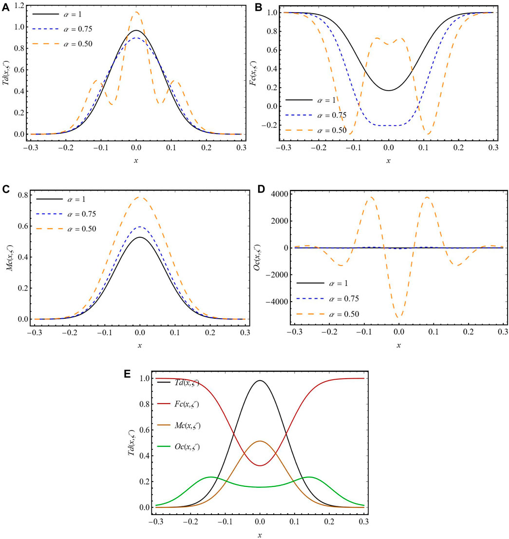
Figure 2. Aquered AAM solution for (A) Td (x, t) (B) Fc (x, t) (C) Mc (x, t) (D) Oc (x, t) (E) Combined surface plot at different alpha values.

Figure 3

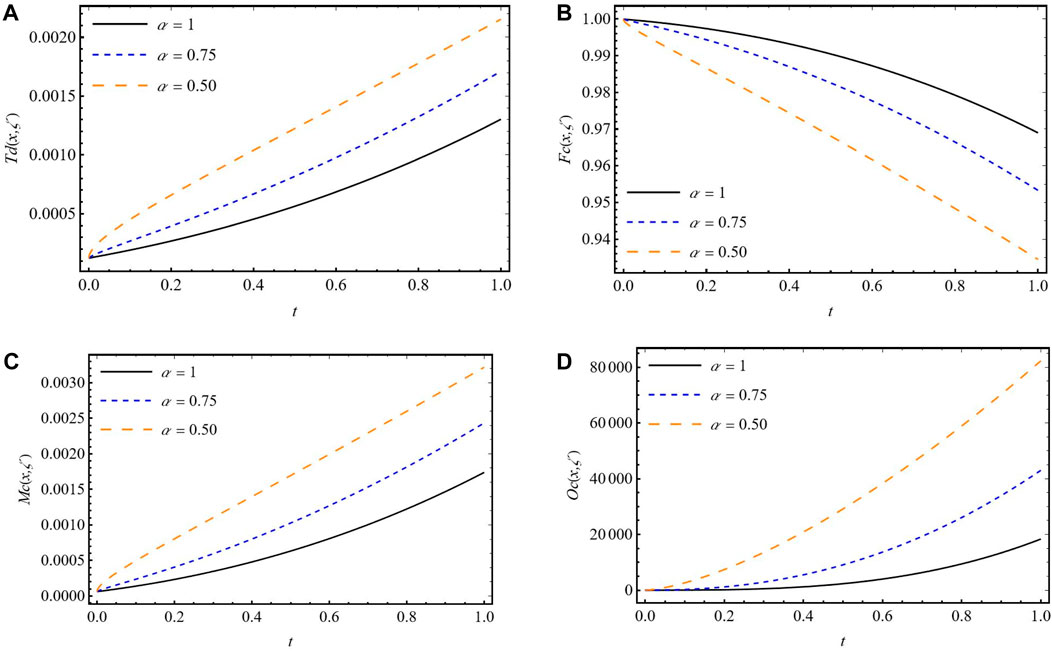
Figure 3. Nature of the solution with respect to time for (A) Td (x, t) (B) Fc (x, t) (C) Mc (x, t) (D) Oc (x, t).

8 Conclusion

The expected analytical solutions for the fractional solid tumor invasion model are studied using an approximate analytical method in the current work. Here, we considered the fractional Caputo derivative to study the considered problem. This method has the potential to be applied to various biological and epidemiological models. The following conclusions can be drawn:

• The uniqueness and existence of the model’s system of solutions with fixed-point theorems are explained.

• The solutions we got using the AAM are in the form of series and converge rapidly.

• The plots indicate a clear influence of both the arbitrary order and the applied parameters on the model.

• The behavior of the model is also dependent on both time instant and time history, which can be easily analyzed by the fractional calculus concept.

• Our analysis confirms that the proposed method is exceptionally efficient and successfully resolves a wide range of non-linear fractional mathematical, biological, and other models.

• The field of mathematical modeling is experiencing a new era with the emergence of fractional calculus.

Data availability statement

The original contributions presented in the study are included in the article/Supplementary Material; further inquiries can be directed to the corresponding author.

Author contributions

HC: conceptualization, data curation, formal analysis, funding acquisition, investigation, methodology, project administration, resources, software, supervision, writing–original draft, and writing–review and editing. RS: conceptualization, data curation, formal analysis, funding acquisition, investigation, methodology, project administration, resources, software, writing–original draft, and writing–review and editing. DP: investigation, methodology, project administration, resources, software, writing–original draft, writing–review and editing, conceptualization, data curation, formal analysis, and funding acquisition. AQ: conceptualization, data curation, formal analysis, funding acquisition, investigation, methodology, project administration, resources, software, writing–original draft, and writing–review and editing. NM: conceptualization, data curation, formal analysis, funding acquisition, investigation, methodology, project administration, resources, software, writing–original draft, and writing–review and editing. MN: conceptualization, data curation, formal analysis, funding acquisition, investigation, methodology, project administration, resources, software, writing–original draft, and writing–review and editing. DS: conceptualization, data curation, formal analysis, funding acquisition, investigation, methodology, project administration, resources, software, writing–original draft, and writing–review and editing.

Funding

The author(s) declare that no financial support was received for the research, authorship, and/or publication of this article.

Conflict of interest

The authors declare that the research was conducted in the absence of any commercial or financial relationships that could be construed as a potential conflict of interest.

Publisher’s note

All claims expressed in this article are solely those of the authors and do not necessarily represent those of their affiliated organizations, or those of the publisher, the editors, and the reviewers. Any product that may be evaluated in this article, or claim that may be made by its manufacturer, is not guaranteed or endorsed by the publisher.

References

1. Mathur P, Sathishkumar K, Chaturvedi M, Das P, Sudarshan KL, Santhappan S, et al. Cancer statistics, 2020: report from national cancer registry programme, India. JCO Glob Oncol (2020) 6:1063–75. doi:10.1200/GO.20.00122

PubMed Abstract | CrossRef Full Text | Google Scholar

2. Russo G, Pepe F, Pisapia P, Palumbo L, Nacchio M, Vigliar E, et al. Microsatellite instability evaluation of patients with solid tumour: routine practice insight from a large series of Italian referral centre. J Clin Pathol (2023) 76(2):133–6. doi:10.1136/jclinpath-2022-208203

PubMed Abstract | CrossRef Full Text | Google Scholar

3. Anderson AR A hybrid mathematical model of solid tumour invasion: the importance of cell adhesion. Math Med Biol (2005) 22(2):163–86. doi:10.1093/imammb/dqi005

PubMed Abstract | CrossRef Full Text | Google Scholar

4. Anderson AR A hybrid multiscale model of solid tumour growth and invasion: evolution and the microenvironment. Single-cell-based Models Biol Med (2007) 3–28. doi:10.1007/978-3-7643-8123-3_1

CrossRef Full Text | Google Scholar

5. Jeon J, Quaranta V, Cummings PT An off-lattice hybrid discrete-continuum model of tumor growth and invasion. Biophysical J (2010) 98(1):37–47. doi:10.1016/j.bpj.2009.10.002

PubMed Abstract | CrossRef Full Text | Google Scholar

6. Kim BK, Kim KA, Park JY, Ahn SH, Chon CY, Han KH, et al. Prospective comparison of prognostic values of modified response evaluation criteria in solid tumours with European association for the study of the liver criteria in hepatocellular carcinoma following chemoembolization. Eur J Cancer (2013) 49(4):826–34.

PubMed Abstract | CrossRef Full Text | Google Scholar

7. Lachowicz M Micro and meso scales of description corresponding to a model of tissue invasion by solid tumours. Math Models Methods Appl Sci (2005) 15(11):1667–83. doi:10.1142/s0218202505000935

CrossRef Full Text | Google Scholar

8. Cristini V, Li X, Lowengrub JS, Wise SM Nonlinear simulations of solid tumor growth using a mixture model: invasion and branching. J Math Biol (2009) 58:723–63. doi:10.1007/s00285-008-0215-x

PubMed Abstract | CrossRef Full Text | Google Scholar

9. Malinzi J, Sibanda P, Mambili-Mamboundou H Analysis of virotherapy in solid tumour invasion. Math Biosciences (2015) 263:102–10.

PubMed Abstract | CrossRef Full Text | Google Scholar

10. Domschke P, Trucu D, Gerisch A, Chaplain MA Mathematical modelling of cancer invasion: implications of cell adhesion variability for tumour infiltrative growth patterns. J Theor Biol (2014) 361:41–60. doi:10.1016/j.jtbi.2014.07.010

PubMed Abstract | CrossRef Full Text | Google Scholar

11. Gerlee P, Anderson AR An evolutionary hybrid cellular automaton model of solid tumour growth. J Theor Biol (2007) 246(4):583–603. doi:10.1016/j.jtbi.2007.01.027

PubMed Abstract | CrossRef Full Text | Google Scholar

12. Byrne HM, King JR, McElwain DS, Preziosi L A two-phase model of solid tumour growth. Appl Maths Lett (2003) 16(4):567–73. doi:10.1016/s0893-9659(03)00038-7

CrossRef Full Text | Google Scholar

13. Lloyd BA, Szczerba D, Rudin M, Székely G A computational framework for modelling solid tumour growth. Philos Trans R Soc A: Math Phys Eng Sci (2008) 366(1879):3301–18. doi:10.1098/rsta.2008.0092

PubMed Abstract | CrossRef Full Text | Google Scholar

14. Nisar KS, Jagatheeshwari R, Ravichandran C, Veeresha P High-performance computational method for fractional model of solid tumour invasion. Ain Shams Eng J (2023) 14:102226. doi:10.1016/j.asej.2023.102226

CrossRef Full Text | Google Scholar

15. Kilbas AA, Srivastava HM, Trujillo JJ Theory and applications of fractional differential equations. Elsevier (2006). p. 204.

Google Scholar

16. Saadeh R, Abu-Ghuwaleh M, Qazza A, Kuffi E A fundamental criteria to establish general formulas of integrals. J Appl Maths (2022) 2022:1–16. doi:10.1155/2022/6049367

CrossRef Full Text | Google Scholar

17. Veeresha P, Prakasha DG An efficient technique for two-dimensional fractional order biological population model. Int J Model Simulation, Scientific Comput (2020) 11(01):2050005. doi:10.1142/s1793962320500051

CrossRef Full Text | Google Scholar

18. Qazza A, Saadeh R, Salah E Solving fractional partial differential equations via a new scheme. AIMS Maths (2022) 8(3):5318–37. ‏. doi:10.3934/math.2023267

CrossRef Full Text | Google Scholar

19. Veeresha P, Gao W, Prakasha DG, Malagi NS, Ilhan E, Baskonus HM New dynamical behaviour of the coronavirus (2019-ncov) infection system with non-local operator from reservoirs to people. Inf Sci Lett (2021) 10(2):17.

Google Scholar

20. Saadeh R, A. Abdoon M, Qazza A, Berir MA. A numerical solution of generalized Caputo fractional initial value problems. Fractal and Fractional (2023) 7(4):332. doi:10.3390/fractalfract7040332

CrossRef Full Text | Google Scholar

21. Area I, Batarfi H, Losada J, Nieto JJ, Shammakh W, Torres A On a fractional order ebola epidemic model. Adv Difference Equations (2015) 2015:278–12. doi:10.1186/s13662-015-0613-5

CrossRef Full Text | Google Scholar

22. Arqub OA, El-Ajou A Solution of the fractional epidemic model by homotopy analysis method. J King Saud University-Science (2013) 25(1):73–81. doi:10.1016/j.jksus.2012.01.003

CrossRef Full Text | Google Scholar

23. Prakasha DG, Veeresha P, Baskonus HM Two novel computational techniques for fractional Gardner and Cahn-Hilliard equations. Comput Math Methods (2019) 1(2):e1021. doi:10.1002/cmm4.1021

CrossRef Full Text | Google Scholar

24. Xu K, Cheng T, Lopes AM, Chen L, Zhu X, Wang M Fuzzy fractional-order PD vibration control of uncertain building structures. Fractal and Fractional (2022) 6(9):473. doi:10.3390/fractalfract6090473

CrossRef Full Text | Google Scholar

25. Saadeh R, Ala’yed O, Qazza A Analytical solution of coupled hirota–satsuma and KdV equations. Fractal nd Fractional (2022) 6(12):694. doi:10.3390/fractalfract6120694

CrossRef Full Text | Google Scholar

26. Amourah A, Alsoboh A, Ogilat O, Gharib GM, Saadeh R, Al Soudi M A generalization of Gegenbauer polynomials and bi-univalent functions. Axioms (2023) 12(2):128. doi:10.3390/axioms12020128

CrossRef Full Text | Google Scholar

27. Alzahrani AB, Abdoon MA, Elbadri M, Berir M, Elgezouli DE A comparative numerical study of the symmetry chaotic jerk system with a hyperbolic sine function via two different methods. Symmetry (2023) 15(11):1991. doi:10.3390/sym15111991

CrossRef Full Text | Google Scholar

28. Salah E, Saadeh R, Qazza A, Hatamleh R Direct power series approach for solving nonlinear initial value problems. Axioms (2023) 12(2):111. doi:10.3390/axioms12020111

CrossRef Full Text | Google Scholar

29. Sontakke BR, Shelke AS, Shaikh AS Solution of non-linear fractional differential equations by variational iteration method and applications. Far East J Math Sci (2019) 110(1):113–29. doi:10.17654/ms110010113

CrossRef Full Text | Google Scholar

30. Ahmad MZ, Alsarayreh D, Alsarayreh A, Qaralleh I Differential transformation method (DTM) for solving SIS and SI epidemic models. Sains Malaysiana (2017) 46(10):2007–17. doi:10.17576/jsm-2017-4610-40

CrossRef Full Text | Google Scholar

31. Momani S, Odibat Z A novel method for nonlinear fractional partial differential equations: combination of DTM and generalized Taylor's formula. J Comput Appl Maths (2008) 220(1-2):85–95. doi:10.1016/j.cam.2007.07.033

CrossRef Full Text | Google Scholar

32. Veeresha P, Prakasha DG, Baskonus HM, Yel G An efficient analytical approach for fractional Lakshmanan-Porsezian-Daniel model. Math Methods Appl Sci (2020) 43(7):4136–55.

CrossRef Full Text | Google Scholar

33. Zhang J, Wei Z, Li L, Zhou C Least-squares residual power series method for the time-fractional differential equations. Complexity (2019) 2019:1–15. doi:10.1155/2019/6159024

CrossRef Full Text | Google Scholar

34. Abdulaziz O, Hashim I, Momani S Solving systems of fractional differential equations by homotopy-perturbation method. Phys Lett A (2008) 372(4):451–9. doi:10.1016/j.physleta.2007.07.059

CrossRef Full Text | Google Scholar

35. Momani S, Odibat Z Homotopy perturbation method for nonlinear partial differential equations of fractional order. Phys Lett A (2007) 365(5-6):345–50. doi:10.1016/j.physleta.2007.01.046

CrossRef Full Text | Google Scholar

36. Baleanu D, Diethelm K, Scalas E, Trujillo JJ Fractional calculus: models and numerical methods. World Scientific (2012) 3.

Google Scholar

37. D’Elia M, Du Q, Glusa C, Gunzburger M, Tian X, Zhou Z Numerical methods for nonlocal and fractional models. Acta Numerica (2020) 29:1–124. doi:10.2172/1598758

CrossRef Full Text | Google Scholar

38. Ahmed H Fractional Euler method; an effective tool for solving fractional differential equations. J Egypt Math Soc (2018) 26(1):38–43. doi:10.21608/joems.2018.9460

CrossRef Full Text | Google Scholar

39. Deng J, Zhao L, Wu Y Fast predictor-corrector approach for the tempered fractional differential equations. Numer Algorithms (2017) 74:717–54. doi:10.1007/s11075-016-0169-9

CrossRef Full Text | Google Scholar

40. Qureshi S, Argyros IK, Soomro A, Gdawiec K, Shaikh AA, Hincal E A new optimal root-finding iterative algorithm: local and semilocal analysis with polynomiography. Numer Algorithms (2023) 95:1715–45. doi:10.1007/s11075-023-01625-7

CrossRef Full Text | Google Scholar

41. Qureshi S, Ramos H, Soomro A, Akinfenwa OA, Akanbi MA Numerical integration of stiff problems using a new time-efficient hybrid block solver based on collocation and interpolation techniques. Mathematics Comput Simulation (2024) 220:237–52. doi:10.1016/j.matcom.2024.01.001

CrossRef Full Text | Google Scholar

42. Uçar S, Evirgen F, Özdemir N, Hammouch Z Mathematical analysis and simulation of a giving up smoking model within the scope of non-singular derivative. Proc Inst Maths Mech (2022) 48:84–99.

Google Scholar

43. Uçar E, Özdemir N A fractional model of cancer-immune system with Caputo and Caputo--Fabrizio derivatives. The Eur Phys J Plus (2021) 136:43–17. doi:10.1140/epjp/s13360-020-00966-9

PubMed Abstract | CrossRef Full Text | Google Scholar

44. Uçar E, Özdemir N, Altun E Qualitative analysis and numerical simulations of new model describing cancer. J Comput Appl Maths (2023) 422:114899. doi:10.1016/j.cam.2022.114899

CrossRef Full Text | Google Scholar

45. Uçar E, Özdemir N New fractional cancer mathematical model via IL-10 cytokine and anti-PD-L1 inhibitor. Fractal and Fractional (2023) 7(2):151. doi:10.3390/fractalfract7020151

CrossRef Full Text | Google Scholar

46. Elsaid A, Abdel Latif MS, Maneea M Similarity solutions for multiterm time-fractional diffusion equation. Adv Math Phys (2016):7304659.

CrossRef Full Text | Google Scholar

47. Elsaid A, Abdel Latif MS, Maneea M Similarity solutions for solving Riesz fractional partial differential equations. Prog Fractional Differ Appl (2016) 2(4):293–8. doi:10.18576/pfda/020407

CrossRef Full Text | Google Scholar

48. Abdel Latif MS, Elsaid A, Maneea M Similarity solutions of fractional order heat equations with variable coefficients. Miskolc Math Notes (2016) 17(1):245–54. doi:10.18514/mmn.2016.1610

CrossRef Full Text | Google Scholar

49. Balzotti C, D’Ovidio M, Loreti P Fractional SIS epidemic models. Fractal and Fractional (2020) 4(3):44. doi:10.3390/fractalfract4030044

CrossRef Full Text | Google Scholar

50. Baishya C, Achar SJ, Veeresha P, Prakasha DG Dynamics of a fractional epidemiological model with disease infection in both the populations. Chaos: Interdiscip J Nonlinear Sci (2021) 31(4):043130. doi:10.1063/5.0028905

CrossRef Full Text | Google Scholar

51. Tassaddiq A, Qureshi S, Soomro A, Arqub OA, Senol M Comparative analysis of classical and Caputo models for COVID-19 spread: vaccination and stability assessment. Fixed Point Theor Algorithms Sci Eng (2024) 2024:2. doi:10.1186/s13663-024-00760-7

CrossRef Full Text | Google Scholar

52. Awadalla M, Alahmadi J, Cheneke KR, Qureshi S Fractional optimal control model and bifurcation analysis of human syncytial respiratory virus transmission dynamics. Fractal and Fractional (2024) 8(1):44. doi:10.3390/fractalfract8010044

CrossRef Full Text | Google Scholar

53. Zafar ZUA, Yusuf A, Musa SS, Qureshi S, Alshomrani AS, Baleanu D Impact of public health awareness programs on COVID-19 dynamics: a fractional modeling approach. FRACTALS (fractals) (2023) 31(10):1–20. doi:10.1142/s0218348x23400054

CrossRef Full Text | Google Scholar

54. Padder A, Almutairi L, Qureshi S, Soomro A, Afroz A, Hincal E, et al. Dynamical analysis of generalized tumor model with Caputo fractional-order derivative. Fractal and Fractional (2023) 7(3):258. doi:10.3390/fractalfract7030258

CrossRef Full Text | Google Scholar

55. Johansyah MD, Sambas A, Qureshi S, Zheng S, Abed-Elhameed TM, Vaidyanathan S, et al. Investigation of the hyperchaos and control in the fractional order financial system with profit margin. Partial Differential Equations Appl Maths (2024) 9:100612. doi:10.1016/j.padiff.2023.100612

CrossRef Full Text | Google Scholar

56. Onder I, Esen H, Secer A, Ozisik M, Bayram M, Qureshi S Stochastic optical solitons of the perturbed nonlinear Schrödinger equation with Kerr law via Ito calculus. Eur Phys J Plus (2023) 138(9):872. doi:10.1140/epjp/s13360-023-04497-x

CrossRef Full Text | Google Scholar

57. Farooq U, Khan H, Tchier F, Hincal E, Baleanu D, Bin Jebreen H New approximate analytical technique for the solution of time fractional fluid flow models. Adv Difference Equations (2021) 2021:81–20. doi:10.1186/s13662-021-03240-z

CrossRef Full Text | Google Scholar

58. Thabet H, Kendre S, Peters J Travelling wave solutions for fractional Korteweg-de Vries equations via an approximate-analytical method. AIMS Maths (2019) 4(4):1203–22. doi:10.3934/math.2019.4.1203

CrossRef Full Text | Google Scholar