Data reduction and processing for photon science detectors

Pennicard, David; Rahmani, Vahid; Graafsma, Heinz

doi:10.3389/fphy.2024.1285854

REVIEW article

Front. Phys., 05 February 2024

Sec. Radiation Detectors and Imaging

Volume 12 - 2024 | https://doi.org/10.3389/fphy.2024.1285854

This article is part of the Research Topic Pushing Frontiers - Imaging For Photon Science View all 18 articles

Data reduction and processing for photon science detectors

David Pennicard¹*

Vahid Rahmani¹

Heinz Graafsma^1,2

¹Deutsches Elektronen-Synchrotron DESY, Hamburg, Germany
²STC research centre, Mid Sweden University, Sundsvall, Sweden

New detectors in photon science experiments produce rapidly-growing volumes of data. For detector developers, this poses two challenges; firstly, raw data streams from detectors must be converted to meaningful images at ever-higher rates, and secondly, there is an increasing need for data reduction relatively early in the data processing chain. An overview of data correction and reduction is presented, with an emphasis on how different data reduction methods apply to different experiments in photon science. These methods can be implemented in different hardware (e.g., CPU, GPU or FPGA) and in different stages of a detector’s data acquisition chain; the strengths and weaknesses of these different approaches are discussed.

1 Introduction

Developments in photon science sources and detectors have led to rapidly-growing data rates and volumes [1]. For example, experiments at the recently-upgraded ESRF EBS can potentially produce a total of a petabyte of data per day, and future detectors targeting frame rates over 100 kHz will have data rates (for raw data) exceeding 1 Tbit/s [2].

These improvements not only allow a much higher throughput of experiments, but also make new measurements feasible. For example, by focusing the beam and raster-scanning it across a sample at high speed, essentially any X-ray technique can be used as a form of microscopy, obtaining atomic-scale structure and chemical information about large samples. But naturally, these increasing data rates pose a variety of challenges for data storage and analysis. In particular, there is increasing demand for data reduction, to ensure that the volume of data that needs to transferred and stored is not unfeasibly large. From the perspective of detector developers, there are two key issues that need to be addressed.

Firstly, the raw data stream from a detector needs to be converted into meaningful images, and this becomes increasingly challenging at high data rates. This conversion process is detector-specific, so implementing it requires detailed knowledge of the detector’s characteristics. At the same time, since the correction process is relatively fixed, there’s a lot of potential to optimize it for performance. In addition, the complexity of this conversion process depends on the detector design, so this is something that should be considered during detector development.

Secondly, it can be beneficial to perform data reduction on-detector, or as part of the detector’s DAQ system. For a variety of reasons, the useful information in a dataset can be captured with a smaller number of bits than the original raw data size; for example, by taking advantage of patterns or redundancy in the raw data, or by rejecting non-useful images in the dataset. In the DAQ system, the data will typically pass through a series of stages, as illustrated in Figure 1; firstly, from the ASIC or monolithic sensor to a custom board in the detector, then to a specialized DAQ PC (or similar hardware), and finally to a more conventional computing environment. By performing data reduction early on in this chain, it is possible to reduce the bandwidth required by later stages. Not only can this reduce the cost and complexity of later stages (especially the cost of data storage), it can also potentially enable the development of faster detectors by overcoming data bandwidth bottlenecks. Performing this early data reduction often ties together with the process of converting the raw data stream to real images, since real images can be easier to compress. Conversely, though, performing data reduction early in the chain can be more challenging, since the hardware in these early stages tends to offer less flexibility, and there are constraints on space and power consumption within the detector.

FIGURE 1

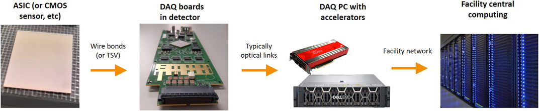
FIGURE 1. Illustration of typical elements in a detector’s DAQ chain.

This paper presents an overview of image correction and data reduction in photon science, with a particular focus on how the characteristics of different detectors and experiments affect the choice of data reduction methods. Section 2 discusses algorithms for converting raw data into corrected images. Section 3 addresses algorithms for data compression, followed by other methods of data reduction (e.g., rejecting bad images) in Section 4. Section 5 provides an overview of standard data-processing hardware such as CPUs, GPUs and FPGAs that can be built into detectors and DAQ systems. Finally, Section 6 brings these elements together, by discussing how data correction and reduction can be implemented at different stages of a detector’s readout and processing chain, and the pros and cons of different approaches.

2 Detector data correction

The raw data stream produced by a detector generally requires processing in order to produce a meaningful image. The steps will of course depend on the design; here, two common cases of photon counting and integrating pixel detectors are considered. Although it can be possible to compress data before all the corrections are applied, corrected data can be more compressible—for example, correcting pixel-to-pixel variations can result in a more uniform image.

Firstly, we want the pixels in an image to follow a straightforward ordering; typically this is row-by-row or column-by-column, though some image formats represent images as a series of blocks for performance reasons. However, data streams from detectors often have a more complex ordering. One reason for this is that data is typically read out from an ASIC or monolithic detector in parallel across multiple readout signal lines which can result in interleaving of data. In addition, in detectors composed of multiple chips or modules, there may be gaps in the image, or some parts of the detector may be rotated—this is illustrated for the AGIPD 1M detector [3] in Figure 2. So, data reordering is a common first step.

FIGURE 2

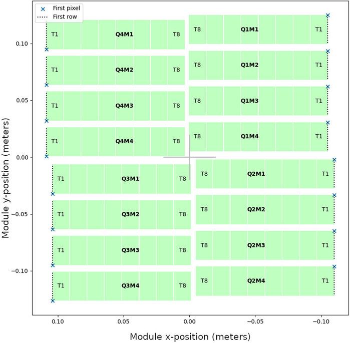
FIGURE 2. Module layout of the AGIPD 1M detector, which has a central hole for the beam, gaps between modules, and different module orientations (with the first pixel of each module indicated by a cross).

In the case of photon counting detectors, the value read out from each pixel is an integer that corresponds relatively directly to the number of photons hitting the pixel. Nevertheless, at higher count rates losses occur due pulse pileup, when photons hit a pixel in quick succession and only one pulse is counted. So, pileup correction is needed, where the hit rate in each pixel is calculated and a rate-dependent multiplicative factor applied. Although there are two well-known models for pileup—paralyzable and non-paralyzable—in practice the behaviour of pixel detectors can be somewhere in-between, and the pulsed structure of synchrotron sources can also affect the probability of pileup [4]. In addition to this some modern detectors have additional pileup compensation, for example, by detecting longer pulses that would indicate pileup [5]. So, the pileup correction model can vary between different detectors.

In integrating detectors, each pixel’s amplifier produces an analog value, which is then digitized. This digitized value then needs to be converted to the energy deposited in the pixel. In many detectors, this is a linear relationship. In experiments with monochromatic beam, each photon will deposit the same amount of energy in the sensor, so it is possible to calculate the corresponding number of photons. The correction process typically consists of the following steps [6, 7]:

• Baseline correction/dark subtraction. As part of the calibration process, dark images are taken with no X-ray beam present and averaged. Then, during image taking, this is subtracted from each new image. This corrects for both pixel-to-pixel variations in the amplifiers’ zero level, and also for the effects of leakage current integrated during image taking. Since this integrated leakage current can vary with factors like integration time, operating temperature and radiation damage in the sensor, new dark images often need to be taken frequently, e.g., at the start of each experiment.

• Common-mode correction. In some detectors, there may be image-to-image variation that is correlated between pixels, for example, due to supply voltage fluctuations. One method for correcting this is to have a small number of pixels that are either masked from X-rays or unbonded, use these to measure this common-mode noise in each image, and then subtract this from all the pixels. Another related effect is crosstalk, where pixels are affected by their neighbours; see for example, Ref. [8] for a discussion of this.

• Gain correction. While integrating detectors are typically designed to have a linear relationship between deposited energy and amplifier voltage, the gain will vary from pixel to pixel, and thus must be measured and corrected for by multiplication.

• “Photonization”. If the incoming X-ray beam is monochromatic, then the measured energy may then be converted to an equivalent number of photons. Up to this point, the correction process is typically performed with floating point numbers, but as discussed later it can be advantageous for compression to round this to an integer number of photons (or alternatively fixed point).

In some integrating detectors designed for large dynamic range, the response may not be a simple linear one. For example, in dynamic gain switching detectors [3, 9] each pixel can adjust its gain in response to the magnitude of the incoming signal, and the output of each pixel consists of a digitized value plus information on which gain setting was used. This increases the number of calibration parameters needing to be measured and corrected, since for each gain setting there will be distinct baseline and gain corrections.

Furthermore, there are a variety of ways in which detectors may deviate from the ideal response, and additional corrections may be required. For example, the response of a detector may not be fully linear, and more complex functions may be need to describe their response. It is also common to treat malfunctioning pixels, for example, by setting them to some special value.

An additional aspect of detector data processing is combining the image data with metadata, i.e., contextual information about images such as their format, detector type, and the experimental conditions under which they were acquired. Some metadata may be directly incorporated into the detector’s data stream. For example, in Free Electron Laser (FEL) experiments the detector needs to be synchronised with the X-ray bunches, and bunches can vary in their characteristics, so each image will be accompanied by a bunch ID, fed to the detector from the facility’s control system. Other metadata may be added later. For example, the NeXuS data format [10] has been adopted by many labs; this is based on the HDF5 format [11], and specifies how metadata should be structured in experiments in photon science and other fields.

3 Data compression and photon science datasets

In general, data compression algorithms reduce the number of bits needed to represent data, by encoding it in a way that takes advantage of patterns or redundancy in the data. These algorithms can be subdivided into lossless compression [12], where the original data can be reconstructed with no error, and lossy compression [13], where there is some difference between the original and reconstructed data. Currently, lossless compression is often applied to photon science data before storage, whereas lossy compression is uncommon, due to concerns about degrading or biasing the results of later analysis. However, lossy compression can achieve higher compression ratios.

The compressibility of an image naturally depends on its content, and in photon science this can vary depending on both the type of experiment and the detector characteristics. In particular, since random noise will not have any particular redundancy or pattern, the presence of noise in an image will reduce the amount of compression that can be achieved with lossless algorithms.

Compared to typical visible light images, X-ray images from pixel detectors can have distinctive features that affect their compressibilty, as discussed further below. Firstly, individual X-ray photons have much greater energy and thus can more easily be discriminated with a suitable detector. Also, X-ray diffraction patterns have characteristics that can make lossless compression relatively efficient. However, imaging experiments using scintillators and visible light cameras produce images more akin to conventional visible light imaging, which do not losslessly compress well.

3.1 Noise in X-ray images, and its effects on compression

Random noise in an image can potentially come from different sources; firstly, electronic noise introduced by the detector, and secondly, inherent statistical variation in the experiment itself.

Any readout electronics will inevitably have electronic noise. However, the signal seen by a detector consists of discrete X-ray photons, and the inherent discreteness of our signal makes it possible to reject the electronic noise, provided that it is small enough to ensure that noise fluctuations are rarely mistaken for a photon. In a silicon sensor without gain, ionizing radiation will generate on average one electron-hole pair per 3.6 eV of energy deposited, e.g., a 12 keV photon will generate approximately 3,300 electrons. In turn, if, for example, we assume the noise is Gaussian with a standard deviation corresponding to 0.1 times the photon energy (330 electrons here) then the probability of a pixel having a noise fluctuation corresponding to 0.5 photons or more would be approximately 1 in 1.7 million [14]. (Common noise sources such as thermal and shot noise discussed below are Gaussian, or approximately so, though other noise sources such as fluctuations in supply voltage may not be.)

When using an integrating detector to detect monochromatic X-rays, then it is possible to convert the integrated signal to an equivalent number of photons in postprocessing as described above. Given sufficiently low noise, this value can be quantized to the nearest whole number of photons to eliminate electronic noise. In photon counting detectors, a hit will be recorded in a pixel if the pulse produced by the photon exceeds a user-defined threshold; once again, if noise fluctuations exceeding the threshold are rare, we will have effectively noise-free counting.

In both cases, the electronic noise in a pixel will be dependent on the integration time for an image, or the shaping time in the case of a photon-counting detector. There are two main competing effects here. On the one hand, for longer timescales, the shot noise due to fluctuations in leakage current will be larger. Conversely, to achieve shorter integration times or shaping times, a higher amplifier bandwidth is required, and this will increase the amount of thermal noise detected [15]. Thermal noise is the noise associated with random thermal motion of electrons, which is effectively white noise.

In addition to electronic noise, however, the physics of photon emission and interaction are inherently probabilistic, and so even if an experiment were repeated under identical conditions there would be statistical fluctuations in the number of photons impinging on each pixel. These fluctuations follow Poisson statistics, and if the expected number of photons arriving in a pixel during a measurement is N, then the standard deviation of the corresponding Poisson distribution will be $\sqrt{N}$ . On the one hand, this can make it easier to develop “low noise” detectors; provided the detector noise for a given photon flux is significantly smaller than $\sqrt{N}$ , then it will have little effect on the final result. However, this makes the data less compressible with lossless algorithms, since random noise introduces variation in the image that is not patterned or redundant. (As discussed later, quantizing pixel values with a variable step size, increasing with $\sqrt{N}$ , can be a way of achieving lossy compression.)

3.2 Applying lossless compression to diffraction data

As noted above, data compression relies on patterns or redundancy in data, and this will vary depending on the experiment. Diffraction patterns differ from conventional images in a variety of respects, with the pattern being mathematically related to the Fourier transform of the object. An example of a diffraction pattern from macromolecular crystallography is shown in Figure 3.

FIGURE 3

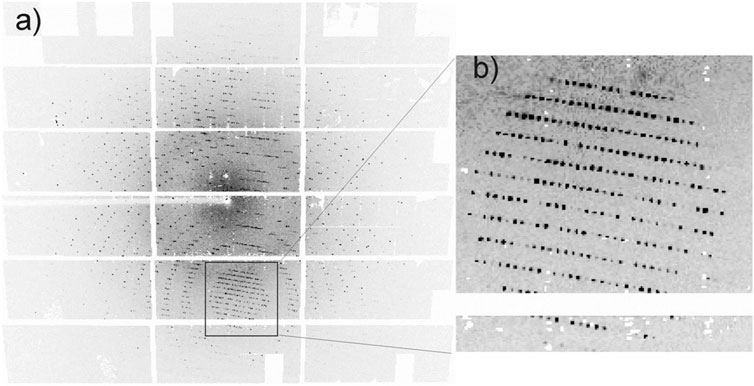
FIGURE 3. A diffraction pattern from a thaumatin crystal, recorded with a Pilatus 1M detector, showing (A) the full detector and (B) a zoom-in of Bragg spots. Reproduced from [16] with permission of the International Union of Crystallography.

Diffraction patterns tend to have various features that are advantageous for lossless compression:

• Hybrid pixel detectors with sensitivity to single photons are the technology of choice for these experiments, making the measurement effectively free from electronic noise as described above. (Detectors for X-ray diffraction require high sensitivity, but pixel sizes in the range of 50–200 μm are generally acceptable.)

• The intensity values measured in the detector typically have a nonuniform distribution, with most pixels measuring relatively low or even zero photons, and a small proportion of pixels having higher values. This is partly because the diffracted intensity drops rapidly at higher scattering angles, and partly because of interference phenomena that tend to produce high intensity in certain places, e.g., Bragg spots or speckles, and low intensity elsewhere.

• Depending on the experiment, nearby pixels will often have similar intensities; for example, in single-crystal diffraction experiments with widely-spaced Bragg spots, the background signal between the spots tends to be smoothly varying.

• Combining these points, in images with fewer photons, there can be patches in the image with many neighbouring zero-value pixels.

Empirically, a range of lossless compression algorithms can achieve good results with diffraction data, especially in high-frame-rate measurements where the number of photons per image will tend to be lower. Experiments applying the DEFLATE [17] algorithm used in GZIP to datasets acquired with photon counting detectors running at high speed showed compression ratios of 19 for high-energy X-ray diffraction, 70 for ptychography and 350 for XPCS experiments with dilute samples (where most pixel values are zero) [18]. Experiments with the Jungfrau integrating detector, applying different compression algorithms to the same data, found that multiple compression methods such as GZIP, LZ4 with a bitshuffle filter and Zstd gave similar compression ratios to one another, but varied greatly in speed, with GZIP being a factor of 10 slower [19].

3.2.1 Example—lossless compression with DEFLATE (GZIP) and Bitshuffle/LZ4

As illustrative examples, we consider the DEFLATE algorithm used in GZIP [20], and the Bitshuffle/LZ4 algorithm [21], firstly to discuss how they take advantage of redundancy to compress diffraction data, and secondly how algorithms with different computational cost can achieve similar performance.

DEFLATE [17] consists of two stages. Firstly, the LZ77 algorithm [22] is applied to the data. This searches for recurring sequences of characters in a file (such as repeated words or phrases in text, or long runs of the same character) and encodes them efficiently, as follows: in the output, the first instance of a sequence of characters is written in full, but then later instances are replaced with special codes referring back to the previous instance. In diffraction datasets, long recurring sequences of characters are generally rare, but there is one big exception; long runs of zeroes. So, the pattern-matching in LZ77 will efficiently compress long runs of zeroes, but the computational work the algorithm does to find more complex recurring sequences is largely wasted.

Secondly, DEFLATE takes the output of the LZ77 stage, and applies Huffman coding [23] to it. Normally, different characters in a dataset (e.g., integers in image data) are all represented with the same number of bits. Huffman coding looks at the frequencies of different characters in the dataset, and produces a new coding scheme that represents common characters with shorter sequences of bits and rare ones with longer sequences. This is analogous to Morse code, where the most common letter in English, “E”, is represented by a single dot, whereas rare letters have longer sequences. For diffraction data, this stage will achieve compression due to the nonuniform statistics of pixel values, where low pixel values are much more common than high ones.

As a contrasting example, the Bitshuffle LZ4 algorithm [21] implicitly takes advantage of the knowledge that the higher bits of pixel values are mostly zero and strongly correlated between neighbouring pixels. In the first step, Bitshuffle, the bits in the data stream are rearranged so that the first bit from every pixel are all grouped together, then the second bit, etc. After this regrouping, the result will often contain long runs of bytes with value zero, as illustrated in Figure 4. The LZ4 algorithm, which is similar to LZ77, will then efficiently encode these long runs of 0 bytes. As mentioned above, this algorithm gives similar performance to GZIP for X-ray diffraction data while being less computationally expensive.

FIGURE 4

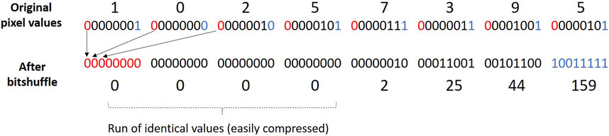
FIGURE 4. Illustration of the Bitshuffle process, used in Bitshuffle/LZ4. This reorders the bits in the data stream so that the LZ4 compression stage can take advantage of the fact that the upper bits in diffraction data are mostly zero, and strongly correlated between neighbouring pixels.. (Eight pixels with 8-bit depth are shown here, but the procedure may be applied to different numberes of pixels and bits.)

3.3 Applying lossy compression to imaging data

While lossless compression can achieve good compression ratios for diffraction data, there is increasing demand for lossy data compression. Firstly, data from some experiments such as imaging do not losslessly compress well, due to noise, and secondly, the increasing data volumes produced by new detectors and experiments mean that higher compression ratios are desirable. The key challenge of lossy compression is ensuring that the compression does not significantly change the final result of analysis. This requires evaluating the results of the compression with a variety of datasets, either by directly comparing the compressed and uncompressed images with a metric of similarity, or by performing the data analysis and applying some appropriate metric of quality to the final result.

In X-ray imaging and tomography experiments, the detector measures X-ray transmission through the sample, and perhaps also additional effects such as enhancement of edges through phase contrast. This means that most pixels will receive a reasonably high X-ray flux, in contrast to X-ray diffraction where most pixels see few or even zero photons. So, noise due to Poisson statistics will be relatively high in most pixels. Likewise, a key requirement for detectors in these experiments is a small effective pixel size (particularly for micro- and nano-tomography), whereas single photon sensitivity is less critical. To achieve this, a common approach is to couple a thin or structured scintillator to a visible light camera with small pixels such as a CMOS sensor or CCD [24]. Magnifying optics may be used to achieve a smaller effective pixel size [25]. This means that the detector noise is also non-negligible.

Since an X-ray transmission image is a real-space image of an object, and broadly resembles a conventional photograph (unlike a diffraction pattern), widely-used lossy compression algorithms for images can potentially be used for compression. In particular, JPEG2000 [26] is already well-established in medical imaging, and in tomography at synchrotrons it has been demonstrated to achieve a factor of three to four compression without significantly affecting the results of the reconstruction [27]. To test this, the reconstruction of the object was performed both before and after compression, and the two results compared using the Mean Structural Similarity Index Measure (MSSIM) metric. A compression factor of six to eight was possible in data with a high signal-to-noise ratio.

3.3.1 Example—lossy compression with JPEG2000

One common approach to both lossy and lossless compression is apply a transform to the data that results in a sparse representation, i.e., most of the resulting values are low or zero. (The choice of transform naturally depends on the characteristics of the data.) The sparse representation can then be compressed efficiently.

In the case of JPEG2000 [26], the Discrete Wavelet Transform [28] is used; in effect, this transformation represents the image of a sum of wave packets with different positions and spatial frequencies. This tends to work well for real space images, which tend to consist of a combination of localized objects and smooth gradients, which can be found on different length scales. After applying the transform, the resulting values are typically rounded off to some level of accuracy, allowing for varying degrees of lossy compression. (By not applying this rounding, lossless compression is also possible.) Then, these values are encoded by a method called arithmetic coding, which is comparable to Huffman coding; it achieves compression by taking advantage of the nonuniform statistics of the transformed values, which in this case are mostly small or zero.

JPEG2000 can be compared with the older JPEG standard, where the transformation consists of splitting the image into 8 × 8 blocks, and applying the Discrete Cosine Transform to each block, thus taking advantage of the fact that images tend to be locally smooth. This is computationally cheaper than most JPEG2000 implementations, but one key drawback is that this can lead to discontinuities between these 8 × 8 blocks after compression. Additionally, JPEG is limited to 8-bit depth (per colour channel) which is unsuitable for many applications, whereas JPEG2000 allows different bit depths. Recently, a high-throughput implementation of JPEG2000 has been developed, HTJ2K [29], with similar speed performance to JPEG. (This is compatible with the JPEG2000 standard but lacks certain features that are not important to scientific applications.)

3.4 Novel methods for lossy compression

As mentioned previously, increasing data volumes mean there is demand for achieving increasing compression, even for experiments such as X-ray diffraction where lossless compression works reasonably well. Naturally, this can be approached by testing a variety of well-established lossy compression algorithms on data, and experimenting with methods such as rounding the data to some level of accuracy. However, there are also new lossy compression methods being developed specifically for scientific data. One particular point of contrast is that most image compression algorithms focus on minimizing the perceptible difference to a human viewer, whereas for scientific data other criteria can be more important, such as imposing limits on the maximum error allowed between original values and compressed values.

One simple example is quantizing X-ray data with a step size smaller than the Poisson noise, which is proportional to $\sqrt{N}$ . For ptychography, for example, it has been demonstrated that quantizing pixel values with a step size of $0.5 \times \sqrt{N}$ [30] does not degrade the quality of the reconstruction.

A more sophisticated example of error-bounded lossy compression is the SZ algorithm [31], which is a method for compressing a series of floating-point values. For each new element in the series, the algorithm checks if its value can be successfully “predicted” (within a specified margin of error) using any one of three methods: directly taking the previous value; linear extrapolation from the previous two values; or quadratically extrapolating from the previous three values. If so, then the pixel value is represented by a 2-bit code indicating the appropriate prediction method. If not, then this “unpredictable” value needs to be stored explicitly. This is illustrated in Figure 5. After the algorithm runs, further compression is applied to the list of unpredictable values.

FIGURE 5

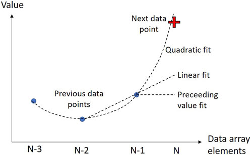
FIGURE 5. Illustration of the “predictive” approach used in SZ compression of floating-point data. If the value of the next data point can be extrapolated (within a user-defined margin of error) from previous data points using one of 3 methods, the point is represented by a 2-bit code indicating the method, e.g., quadratic in this case.

Reference [32] reports on applying SZ to serial crystallography data from LCLS, where the images consist of floating point values obtained from an integrating detector. In this method, lossless compression is applied to regions of interest consisting of Bragg peaks detected in the image, while binning followed by lossy compression is applied to the rest of the image, with the goal of ensuring that any weak peaks that went undetected will still have their intensities preserved sufficiently well. It is reported that when using this strategy, using SZ for the lossy compression can achieve a compression ratio of 190 while still achieving acceptable data quality, whereas other lossy compression methods tested gave a compression ratio of 35 at best.

4 Other forms of data reduction

The data compression methods discussed thus far work by representing a given file using fewer bits; the original file can be reconstructed from the compressed file, albeit with some inaccuracy in the case of lossy compression. More broadly, though, there are other methods of data reduction which rely on eliminating non-useful data entirely, or which transform or process the data in a non-recoverable way. These methods have the potential to greatly reduce the amount of data needing to be stored, though of course it is crucial to establish that these methods are reliable before putting them into practice. In recent years, there has been increasing research into using machine learning for both rejecting non-useful data and for data processing. This includes supervised learning methods, where an algorithm learns to perform a task using training data consisting of inputs and the corresponding correct output, and unsupervised learning methods, which can discover underlying patterns in data.

4.1 Data rejection/vetoing

In some experiments, a large fraction of the data collected does not contain useful information. For example, in experiments at FELs such as serial crystallography and single particle imaging, the sample can consist of a liquid jet containing protein nanocrystals or objects such as viruses passing through the path of the beam. However, only a small fraction of X-ray pulses (in some cases, of order 1%) actually hit a sample to produce an image containing a useful diffraction pattern. So, in these kind of experiments, data volumes can be greatly reduced by rejecting images where the beam did not hit the target.

A variety of methods have been developed for doing this. In serial crystallography, images where the beam hit a crystal will contain Bragg peaks, whereas miss images will only have scattering from the liquid jet. So, a common approach is to search for Bragg peaks in each image, and only accept images where the total number of peaks exceeds some threshold value; this approach is used in software such as Cheetah [33] and DIALS [34]. Since X-ray diffraction intensity varies with scattering angle, these methods often rely on estimating the background signal in the surrounding area of the image when judging whether a peak is present or not.

Machine learning techniques have also been applied to this task, where supervised learning is used to distinguish between good and bad images [35–38]. Supervised learning relies on having training data consisting of input images and the corresponding correct output. This data is used to train a model, such as a neural network; after this, the model can be used to classify new images. In some cases, the training data may consist of simulated data, or images from experiments that have been classified as good or bad by an expert. In this case, the appeal of machine learning is that it makes it possible to distinguish between good and bad images in cases where there is no known algorithm for doing so. Alternatively, the training data may consist of known good and bad images from previous experiments that have been classified by a pre-existing algorithm. In this case, machine learning can potentially improve on the algorithm by being less computationally intensive or by requiring less fine-tuning of algorithm parameters.

As an example, one common approach to image classification is deep learning using convolutional neural networks (CNNs) [39]. For neural networks, the training process consists of feeding input examples into the network, comparing the resulting outputs to the expected correct outputs, and adjusting the network’s parameters through a process called backpropagation in order to improve the network’s performance. CNNs are a special type of network suitable for large, structured inputs like images. As shown in Figure 6, they have a series of convolutional layers; each layer consists of an array of identical neurons, each looking at small patch of the image. These layers learn to recognise progressively higher-level features in the image. Finally, fully-connected layers of neurons use these high-level features to classify the image. An example of using CNNs to categorize images in serial crystallography found in Ref. [36].

FIGURE 6

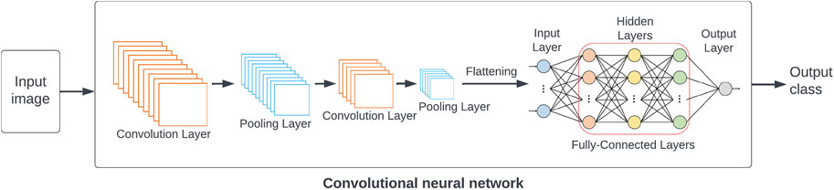
FIGURE 6. The structure of a Convolutional Neural Network (CNN) for image classification.

While machine learning is a rapidly-growing field with great potential, these techniques also have limitations. Firstly, substantial amounts of labelled training data are needed. Secondly, systematic differences between training data and new data may result in a failure to generalise to the new data; as a result, it is often necessary to test and retrain models. Furthermore, even if a machine learning algorithm works successfully, it is often not transparent how it works, making it difficult to understand and trust.

The strategy of vetoing uninteresting data is already well-established in particle physics collider experiments, where only a tiny fraction of collisions will produce particles that are interesting to the experimenter. The data from each collision is temporarily buffered, a subset of this data is read out, and this is used to make a decision on whether to read out the full event [40]. The need for triggering has driven the development of real-time data processing with short latencies [41] and the development of machine learning methods [42]; photon science can potentially benefit from this. However, compared to particle physics, vetoing in photon science faces the challenge that there can be a lot of variation between different beamlines and user experiments, and there is generally less a priori knowledge or simulation of what interesting or uninteresting data will look like.

4.2 Data reduction by processing

Often, the final result of data analysis is much more compact than the original dataset; in determining a protein structure, for example, the data may consist of tens of thousands of diffraction images, while the resulting structure can be described as a list of atomic positions in the molecule.

In some cases the full analysis of a dataset by the user may take months or years, and a lot of this analysis is very experiment-specific, so this is not suitable for achieving fast data reduction close to the detector. Nevertheless, there can be initial processing steps that are common to multiple experiments and which could be applied quickly as part of the DAQ system.

One example of this is azimuthal integration. In some X-ray diffraction experiments, such as powder diffraction, the signal on the detector has rotational symmetry, and so the data can be reduced to a 1-D profile of X-ray intensity as a function of diffraction angle. For a multi-megapixel-sized detector, this corresponds to a factor of 1,000 reduction in data size. Hardware-accelerated implementations of azimuthal integration have been developed for GPUs [43], and more recently for FPGAs [44]. Another example is the calculation of autocorrelation functions in XPCS. In this technique, the dynamics of fluids can be studied from the fluctuations in speckle patterns produced by a coherent X-ray beam. Data processing consists first of calculating a per-pixel-correlation function from a large stack of images over time, and then averaging as a function of scattering angle. FPGA implementations are discussed in Ref. [45].

This is also an area where there is the potential to use machine learning. Firstly, data processing algorithms can be computationally expensive and time-consuming, especially if they involve an iterative reconstruction process. Supervised machine learning can potentially find a computationally-cheaper way of doing this, using experimental data and the results of the existing reconstruction method as the training data. For example, a neural network has been developed for extracting the structure of FEL pulses from gas-based streaking detectors, which would normally require iteratively solving a complex system of equations [46]. In this particular case, the neural network was implemented in an FPGA, in order to achieve low latency.

Additionally, unsupervised machine learning could potentially be used to extract information from X-ray data. These methods require training data, but unlike supervised learning only input data is needed, not information on the “correct” output. For example, variational autoencoders [47] learn to reduce complex data such as images to a vector representing their key features. This approach has been applied to X-ray diffraction patterns obtained from doped crystals, and it was found that the features extracted by the autoencoder could be used to determine the doping concentration [48].

4.3 Connections between data reduction and on-the-fly analysis

At light sources, there is a move towards performing on-the-fly data analysis, where data from the experiment is streamed to a computing cluster and analysed immediately [49]. This can provide immediate feedback to the user to guide the experiment and make data taking more efficient; for example, by allowing users to quickly identify the most useful samples to study, or regions of interest within a sample that can be investigated in more detail [50].

If data reduction close to the detector involves performing analysis steps on data (e.g., azimuthal integration) or makes the data easier to process (e.g., making the dataset smaller by rejecting bad data) then this synergises with on-the-fly data processing, by reducing the workload on the computing cluster.

Typically, these sort of data reduction methods have the drawback that if some or all of the original data is discarded, then any errors in the processing cannot be corrected. For example, performing azimuthal integration correctly requires accurate calibration of the centre of the diffraction pattern and any tilt of the detector relative to the beam.

However, since on-the-fly data analysis is useful to users, the trustworthiness of these methods can be established in stages. For example, as a first stage all the raw data may be saved to disk for later analysis, with on-the-fly processing providing quick feedback during the experiment. Once the reliability of the automatic processing is better-established, raw data might only be stored for a shorter time before deletion (or transfer to cheaper storage such as tape) to give the opportunity for the user to cross-check for correctness. Finally, once the on-the-fly data processing is fully trusted, it may be possible to only save a small fraction of the raw data for validation purposes.

5 Overview of data processing hardware

“Off the shelf” data processing hardware such as CPUs, GPUs and FPGAs play a key role in building data acquisition systems for detectors. These components can be used in various places in the detector and DAQ system, and in some cases a combination of these can be used. For example, even custom hardware such as a circuit board for detector control will likely incorporate a microcontroller with a CPU, an FPGA, or a System-On-Chip containing both of these.

Here, we give an overview of the distinctive features of CPUs, GPUs and FPGAs for data processing. In particular, a major aspect of high-performance computing is parallelization of work, where a data processing task is divided between many processing units, but how this is achieved varies between devices, which can affect the best choice of hardware for the task. (How these different types of hardware can be incorporated into a detector system is discussed later, in Section 6.) As an illustrative example [51], compares CPUs, GPUs and FPGAs for image processing tasks. For all the tasks studied, either the GPU, the FPGA or both offered around an order of magnitude higher speed than CPU, but which one was better depended on the task; for example, GPUs performed much better than FPGAs for image filtering with small filter size, whereas FPGAs were better for stereo vision.

In addition to these, a variety of new hardware accelerators aimed at machine learning have been developed. These vary in architecture, but some examples of these are discussed in Subsection 5.4. Lastly, in recent years there have also been efforts to incorporate data processing directly into detector ASICs. This is discussed later on, in 6.1, since this is detector-specific processing.

5.1 CPUs—central processing units

The architecture of a typical CPU [52] is shown in Figure 7. A key feature of modern CPUs is that they’re designed to be able to run many different programs in a way that appears simultaneous to the user. Most modern CPUs are composed of a number of cores; for example, CPUs in the high-end AMD EPYC series have from 32 to 128, though desktop PCs typically have 2–6. Each core has a control unit, which is able to independently interpret a series of instructions in software and execute them, along with an arithmetic unit for performing operations on data, and cache memory for temporarily storing data. Furthermore, CPUs cores can very rapidly switch between executing different tasks, so even a single CPU core can perform many tasks in a way that seems parallel to the user. In most cases, the CPU will be running an operating system, which handles the sharing of resources such as memory and peripherals between the tasks in a convenient way for programmers. High performance computing with CPUs generally involves parallelization of work across multiple cores; in doing this, the different cores can operate relatively independently. For illustration, a detailed example of optimizing CPU code for the widely-used Fast Fourier Transform algorithm can be found in Ref. [53], which compares three different multithreaded packages for this.

FIGURE 7

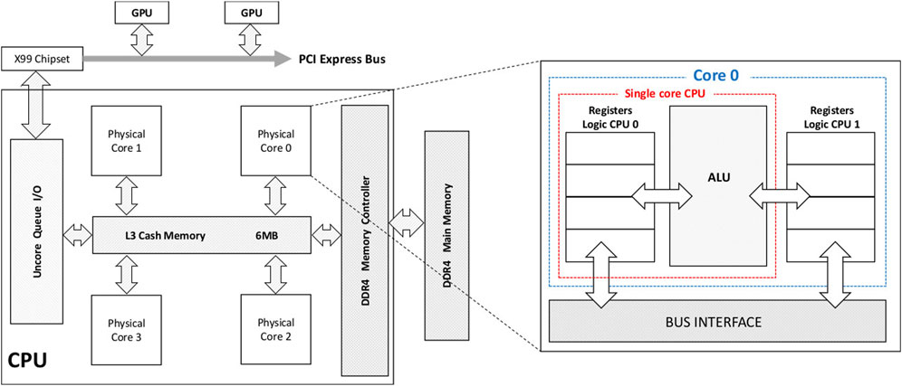
FIGURE 7. Example of a typical CPU’s architecture, showing a device with four cores and hyperthreading capability. Connections to other devices such as main memory (DDR4) and a GPU are also shown [52].

Compared to GPUs and FPGAs, CPUs are generally the easiest to use and program. Indeed, GPUs are virtually always used as accelerator cards as part of a system with a CPU, and it is common for systems based on FPGAs to make use of a CPU (e.g., as part of a System On Chip). In addition, if a task is inherently sequential and cannot be parallelized, then a CPU core may give better performance than a GPU or FPGA. However, CPUs generally have much less parallel processing power than GPUs or FPGAs.

5.2 GPUs—graphics processing units

GPUs are designed to allow massively parallel processing for tasks such as graphics processing or general-purpose computing. The basic units of GPUs are called CUDA cores (in NVIDIA GPUs) or stream processors (in AMD GPUs). These are much more numerous than CPU cores, numbering in the thousands, allowing much greater parallelism and processing power. However, rather than each core being able to independently interpret a stream of instructions, these cores are organised into blocks, with all the cores in a block simultaneously executing the same instruction on different data elements - for example, applying the same mathematical operation to different elements in an array [54]. The structure of a typical GPU is shown in Figure 8.

FIGURE 8

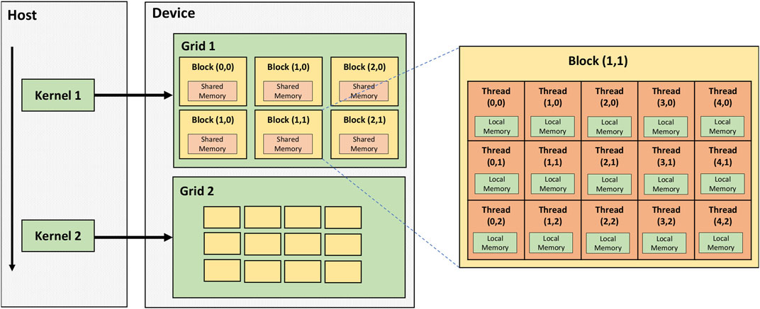
FIGURE 8. Architecture of an NVIDIA GPU (labelled “device”) connected to a PC (“host”). The basic processing units on the GPU are called threads, which are organised into blocks; all the threads in a block will perform the same operation on different data in lockstep. In turn, a given task (kernel) will be performed on a grid consisting of multiple blocks [54].

GPU programming relies on specialized frameworks such as CUDA [55], which was specifically developed for NVIDIA GPUs, or OpenCL [56], an open framework supporting a range of devices that also includes CPUs and FPGAs. GPUs are generally used as accelerator cards in a system with a CPU, and these frameworks firstly allow the CPU to control the GPU’s operation (by passing data to and from it, and starting tasks) and secondly to program functions that will run on the GPU. Typically, GPU code contains additional instructions controlling how different GPU cores in a block access data; e.g., when performing an operation on an array, the first core in a block might perform operations on the first element, and so forth. This can be relatively easy to apply to a lot of image processing tasks, where each processing step can be applied to pixels relatively independently, but GPU implementation can be more challenging for some compression algorithms that act sequentially on data.

GPUs have been shown to perform well for many commonly-used algorithms such as matrix multiplication and Fourier transforms—for example, achieving an order of magnitude speed improvement in performing a Fast Fourier Transform [57]. In particular, GPUs are widely used for training and inference in machine learning in photon science [58–60]. Some newer models of GPU are specially optimized for machine learning applications [61]. For example, neural network calculations typically consist of multiplying and adding matrices, and new GPUs can have specialised cores for this.

5.3 FPGAs—field programmable gate arrays

FPGAs are a type of highly configurable hardware. As shown in Figure 9, within an FPGA there are many blocks providing functionality such as combinatorial logic, digital signal processing and memory, with programmable interconnects between them [62]. While software for a GPU or CPU consists of a series of instructions for the processor to follow, an FPGA’s firmware configures the programmable interconnects to produce a circuit providing the required functionality. The large number of blocks in an FPGA can then provide highly parallel processing and high throughput of data.

FIGURE 9

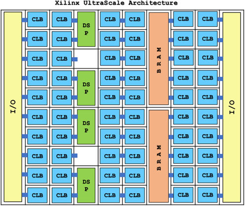
FIGURE 9. Illustration of the internal architecture of a Xilinx UltraScale FPGA. The FPGA consists of an array of blocks such as I/O (input and output), Combinatorial Logic Blocks, Digital Signal Processing and memory in the form of SRAM, which can be flexibly configured [62].

Traditionally, firmware is developed by using a hardware description language to describe the required functionality; a compiler then finds a suitable configuration of blocks and interconnects to achieve this. While hardware description languages differ substantially from conventional programming languages, high-level-synthesis tools for FPGAs have been more recently developed to make it possible to describe an algorithm with a more conventional programming language such as C++, with special directives in the code being used to indicate how parallelism can be achieved with the FPGA.

A distinctive form of parallelism in FPGAs is pipelining. A series of processing steps will often be implemented as a series of blocks forming a pipeline, with data being passed along from one block to another. This is analogous to a production line in a factory, where each station carries out a particular fabrication step, and goods pass from one station to another. As with the production line, at any given moment there will be multiple data elements in different stages of processing being worked on simultaneously. In turn, to make algorithms run efficiently in an FPGA, they need to be designed to make effective use of this pipeline parallelism. This means that FPGAs tend to be better-suited to algorithms that operate on relatively continuous streams of data, rather than algorithms that rely on holding large amounts of data in memory and accessing them in an arbitrary way. As well as achieving a high throughput, algorithms on FPGA can give a reliably low latency, which can be important in cases where fast feedback is required. However, it is generally more challenging to program FPGAs than CPUs or GPUs.

In photon science, FPGAs have been used, for example, for performing autocorrelation in XPCS experiments [45] and azimuthal integration [44]. For machine learning, libraries are becoming available to make it easier to perform inference with neural networks on FPGAs [63]. Additionally, FPGA vendors have developed devices aimed at machine learning [64]; provides an evaluation of Xilinx’s Versal platform, which, for example, includes “AI engines” for running neural networks.

5.4 AI accelerators

In recent years, a range of accelerators have been developed for machine learning. Examples of these include Intelligence Processing Units from Graphcore, and the GroqChip from Groq; an overview of some of these can be found in Ref. [65].

While these have varied architectures, they typically have certain features aimed at implementing neural networks efficiently. A neuron’s output is a function of the weighted sum of its inputs, so AI accelerators are designed to perform many multiply-and-accumulate operations efficiently. They typically have large amounts of on-chip memory, in order to accommodate the high number of weights in a big neural network. Additionally, these accelerators can use numerical formats that are optimised for machine learning. For example, BFLOAT16 [66] is a 16-bit floating point format which covers the same range as standard IEEE 32-bit floating point but with lower precision; this is still sufficient for many neural networks, but makes calculations computationally cheaper.

These kinds of accelerator have recently been investigated for photon science applications. For example, in Ref. [67] a neural network for processing FEL pulse structure information from a streaking detector was implemented both for NVidia A100 GPUs and Graphcore IPUs. This was a convolutional network with encoder and decoder stages that could be used both to denoise the data and to extract latent features. Inference on the IPUs was roughly an order of magnitude faster than on GPUs, and training time was also significantly improved.

6 Data transfer and processing chains in detectors

A typical detector and DAQ system consist of series of stages, as illustrated previously in Figure 1. At each stage, data transfer is needed, and we face a series of bottlenecks which can limit the possible data rate. By doing data reduction earlier on in this chain, the data transfer demands on later stages are reduced, and we can take advantage of this to achieve higher detector speeds. Conversely, the hardware used in earlier stages of this chain is typically more “custom” or specialized, making the implementation of data reduction more challenging, and typically there is also less flexibility in these stages.

The stages in the readout and processing chain are as follows, and the potential for data reduction at each stage will be discussed in more detail in the following section.

• The readout chip (hybrid pixel) or monolithic sensor.

• Readout electronics within the detector itself, which typically incorporate an FPGA, microcontroller or similar.

• Detector-specific data processing hardware. Typically, this consists of one or more PCs, which can include peripherals such as FPGAs or GPUs, but it is also possible to build more specialized systems, such as crates of FPGA boards.

• Generic high-performance-computing hardware, typically in the facility’s computing cluster.

Please note that this discussion focuses on data processing and reduction “close to the detector”, rather than a facility’s full data analysis and storage system. Further information on this broader topic is available, for example, in publications on the newly-built LCLS-II data system [68] and an overview of big data at synchrotrons [69]. Furthermore, the level of data reduction required depends strongly on the costs of data processing and storage downstream. For example, for LCLS-II the goal is to reduce the data volume by at least a factor of 10 for each experiment.

6.1 On-chip data reduction

The first data bottleneck encountered in the detector is transferring data out of the hybrid pixel readout chip or monolithic sensor. In a pixel detector, we have a 2D array of pixels generating data, and within the chip it is possible to have a high density of signal routing; it is common to have a data bus for each pixel column. However, data output takes place across a limited number of transceivers (for example, 16 for the recent Timepix4 chip [70]), which are typically located at the periphery of the chip. These transceivers usually connect to a circuit board via wire bonds, though there is increasing effort in using Through Silicon Vias—TSVs—for interconnect [71]. In turn, further bottlenecks are faced in connecting these to the rest of the readout system. Many X-ray experiments require large continuous detector areas. Typically, these large detectors have a modular design, with each module’s electronics placed behind it. In this situation, achieving high detector frame rates requires building readout electronics with high bandwidth per unit area; the achievable bandwith per unit area then depends both on the performance and physical size of PCB traces and other components [72, 73]. So, performing on-chip data reduction can make it possible to build faster detectors without being limited by these bottlenecks.

Naturally, any circuitry for on-chip compression must be designed to not occupy excessive amounts of space in the pixels or periphery. Additionally, readout chips are developed in technology scales that are relatively large compared to commercial data processing hardware like GPUs and FPGAs, due to the high cost of smaller nodes. Typically, rather than implementing general-purpose processing logic into detector chips, specific algorithms are implemented.

Reference [18] presents a design for on-chip data compression for photon counting detectors, using techniques similar to those discussed previously in Section 3. Firstly, within the pixels, count values are encoded with a varying step size, with the step size getting larger for larger pixel values such that the step does not exceed the $\sqrt{N}$ Poisson noise. This is lossy compression, but the additional noise introduced by this encoding should be less than the Poisson noise. Then, in the chip’s periphery during readout, a lossless compression scheme is applied that bit shuffles the data (much as described for bitshuffle LZ4) then encodes runs of zeroes efficiently. Applied to example datasets, this computationally-cheap approach achieved a compression ratio of around 6 for XRD data, compared to 19 obtained with GZIP.

More recently, lossy on-chip compression methods have been developed using two different algorithms - principal components analysis and an autoencoder [74]. The logic for doing this was distributed throughout the chip, with the analog pixel circuitry consisting of “islands” of 2 × 2 pixels. Applying these algorithms to an image requires prior knowledge about the content of a typical image; in the case of an autoencoder, which is a type of neural network, the neural weights are learned from training data. In this implementation, training was done using ptychography data, and the resulting weights were hard-coded in the chip.

One important limitation of on-chip data compression is that in a large tiled detector composed of multiple chips, the compressibility of the data can vary a great deal between different chips. In X-ray diffraction experiments in particular, the X-ray intensity close to the beam is much higher than at large scattering angles, leading to less compression. So, chips close to the beam may encounter data bottlenecks even if a high overall level of compression is achieved for the detector as a whole.

Another example of on-chip reduction is data vetoing by rejecting bad images, as discussed previously. The Sparkpix-ED chip is one of a family of chips with built-in data reduction being developed by SLAC [75]. It is an integrating pixel detector with two key features. Firstly, each pixel has built-in memory which is used to store recent images. Secondly, there is summing circuitry that can add together the signals in groups of 3 × 3 pixels, to produce a low-resolution image with 1/9 of the size. During operation, each time a new image is acquired the detector will store the full-resolution image in memory and send out the low-resolution image to the readout system. The readout system will then analyse the low-resolution images to see if an interesting event occurred (e.g., diffraction from a protein crystal in a serial crystallography experiment). If so, the detector can be triggered to read out the corresponding full-resolution image from memory; if not, the image will be discarded. A small prototype has demonstrated reading out low-resolution images at 1 MHz frame rate, and full-resolution images at 100 kHz.

6.2 On-detector processing and compression

Data processing and compression can potentially be done within the detector, before data is transferred to the control system (typically over optical links). Once again, this can reduce the bandwidth required for this data transfer.

Typically, on-detector electronics are needed both to control the detector’s operation, and to perform serialization and encoding of data into some standard format so that it can be sent efficiently back to the control system and received using off-the-shelf hardware. (In some cases, it is also necessary to interface to additional components such as on-board ADCs.) One particular benefit of serialization is that individual transceivers on a readout chip typically run at a lower data rate than can be achieved by modern optical links, so serialization can allow these links to be used more efficiently; for example, even the fastest on-chip transceivers typically do not have data rates above 5 Gbit/s, whereas data sent using 100 Gigabit Ethernet with QSFP28 transceivers consists of 4 channels with a data rate of 25 Gbit/s each. These tasks of control and serialization are typically implemented in an FPGA, or a System-On-Chip (SoC) with an FPGA fabric. So, the most common approach to on-detector data processing is to use the FPGA’s processing resources.

As discussed in more detail earlier, FPGAs can provide highly-parallelized data processing, but firmware development can be challenging and time consuming. So, detector-specific processing routines that will always need to be performed on the data are better-suited to FPGA implementation than ones that vary a lot between experiments.

For example, FPGAs in the EIGER photon counting detector perform count-rate correction and image summing [76]. Since the counters in the pixel have a depth of 12 bits, this makes it possible for the detector to acquire images with a depth of up to 32 bits by acquiring a series of images and internally summing them, rather than needing to transfer many 12-bit images to the DAQ system.

One drawback of on-detector processing is that if the FPGA is used for control, serialization and data processing, then it can become more difficult to change the data processing routines. When FPGA firmware is compiled, the compiler will route together blocks in the FPGA to produced the desired functionality. So, changing the data processing routines can change the routing of other functionality in the FPGA, potentially affecting reliability. So, careful re-testing is required after changing the data processing. This is another reason why on-detector processing with FPGAs is mostly used for fixed, detector-specific routines.

6.3 Data acquisition hardware such as PCs with accelerator cards

Data sent out from a detector module will normally be received by either one or more DAQ PCs, or more specialized hardware, located either at the beamline or in the facility’s computing centre. These parts of the DAQ system typically have a range of functions:

• Detector configuration and acquisition control, which requires both monitoring the detector’s state and data output, and receiving commands from the control system.

• Ensuring reliable data reception. It is common for a detector’s output to be a continuous flow of data, transferred by a simple protocol like UDP without the capability to re-send lost packets [77], So the DAQ system is required to reliably receive and buffer this data; this typically requires, for example, having dedicated, high performance network or receiver cards.

• Data correction and reduction.

• Transferring data to where it is needed, for example, the facility’s storage system, online processing and/or a user interface for feedback. This can include tasks like adding metadata and file formatting.

Compared to detectors themselves, these systems tend to be built with relatively off-the-shelf hardware components - for example, standard network cards or accelerator cards. This use of off-the-shelf hardware can reduce the costs of implementing data correction and reduction. In addition, it can be easier to upgrade this hardware over time to take advantage of improvements in technology. These DAQ systems may do processing with conventional CPUs, hardware accelerators such as GPUs and FPGAs, or a mixture of these.

One recent example of this approach is the Jungfraujoch processing system, developed by PSI for the Jungfrau 4-megapixel detector [78]. (A similar approach is taken by the CITIUS detector [79].) The Jungfraujoch system is based on an IBM IC922 server PC, equipped with accelerator cards, and can handle 17 GB/s data when the detector is running at 2 kHz frame rate.

The Jungfraujoch server is shown in Figure 10 (reproduced from [78] with permission of the International Union of Crystallography). Firstly, it is equipped with two “smart network cards” from Alpha Data, each with a Xilinx Virtex Ultrascale + FPGA and a 100 Gigabit Ethernet network link. These receive data directly from the detector over UDP. The FPGA then converts the raw data into images, as described in Ref. [9]. Jungfrau is an integrating detector with gain switching, so the raw data consists of ADC values, and the process of converting this to either photons or energy values includes subtracting the dark current and scaling by an appropriate gain factor. The FPGA also performs the Bitshuffle algorithm, which is the first step in Bitshuffle LZ4 compression described previously; since this algorithm involves reordering bits in a data stream, this is well-suited to implementation on FPGA. The FPGA is primarily programmed by using High Level Synthesis (HLS) based on C++.

FIGURE 10

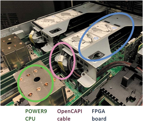
FIGURE 10. A photograph of the IC922 server (IBM) used in Jungfraujoch, showing the FPGA board used for data reception and processing, and the OpenCAPI link allowing coherent access to the CPU’s memory. Reproduced from [78] with permission of the International Union of Crystallography.

The data from each FPGA is transferred to the host server PC using OpenCAPI interconnects, which both allows high speed data transfer at 25 GB/s, and makes it simpler for the FPGA to access memory on the server. The CPU in the server performs the LZ4 part of the Bitshuffle LZ4 lossless compression algorithm, then forwards this data to the file system using ZeroMQ so it can be written to the file system as an HDF5 file. There is also a GPU in the system that can perform tasks such as spot finding in macromolecular crystallography, and monitoring aspects of the detector’s behaviour such as the dark current. (These tasks are well suited to GPUs, since they involve performing operations on full images in parallel.)

One promising technological development in this field is that FPGA and GPU vendors are increasingly developing accelerator cards with built-in network links for the datacenter market. For example, Xilinx have the Alveo line of FPGA cards with two 100 Gigabit Ethernet links and optional high-bandwidth memory, and likewise NVIDIA is currently developing GPU cards with network links. So, this will increase the availability of powerful, standardized hardware for building DAQ systems.

6.4 Computing clusters

Modern light sources are generally supported by large computer clusters for data processing and large storage systems [68]. Data from DAQ PCs or similar hardware at the beamlines can be transferred to them over the facility’s network. Data processing in computing clusters can be divided into online analysis, where the data is transferred directly to the cluster to provide fast results to the experiment, and offine analysis where data is read back from storage for processing at a later point. (Naturally, there may not be a sharp dividing line between these two approaches.) In addition to server PCs with CPUs, computing clusters can also incorporate GPUs or less commonly FPGAs.

In a computing cluster, there is generally a scheduling system that controls how tasks are assigned to the computers. This has the advantage of allowing sharing of resources between different experiments and users according to needs, whereas dedicated hardware installed at a beamline may be idle much of the time. Computing clusters are also much better-suited to allowing users to remotely access to their data and providing the software tools required to analyse it. However, this flexibility in task scheduling and usage can make it more difficult to ensure that we can reliably receive and process images from the detector at the required rate; this is one reason for having dedicated DAQ computers at the beamline for receiving detector data.

7 Conclusion

The increasing data rates of detectors for photon science mean there is a need for high-speed detector data correction, and data reduction.

There are strong ties between these tasks. On the one hand, data reduction can often yield better results on properly-corrected data, since the correction process can reduce spurious variation in images (e.g., pixel-to-pixel variation in response) and make it easier to exploit redundancy in the data. Conversely, after lossy data reduction it is impossible to perfectly recover the original data, so it is crucial to ensure that the quality of the data correction is as good as possible.

Both of these tasks can benefit from making better use of hardware accelerators such as GPUs and FPGAs for highly parallel processing. The increasing use of accelerators in other areas, such as datacenters, means that we can take advantage of improvements in both their hardware and in tools for programming them. In particular, as FPGAs and GPUs with built-in network links become available “off the shelf”, this increases the potential for different labs to build their DAQ systems with compatible hardware, and share the algorithms they develop. Although this paper emphasizes data processing hardware, it is also important to note that well-designed and coded algorithms can deliver much better performance.

Data reduction is a growing field in photon science. To date, lossless compression has mainly been used, since this ensures that there is no loss in data quality, and in some experiments lossless methods can achieve impressive compression ratios. However, lossless compression is relatively ineffective for methods such as imaging, and as data volumes increase there is demand for even greater data reduction in diffraction experiments. So, there will be an increasing need for lossy compression and other methods of reduction. In doing so, it is crucial to use appropriate metrics to test that the data reduction does not significantly reduce the quality of the final analysis. By using well-established methods of lossy compression, for example, image compression with JPEG2000, it is easier to incorporate data reduction into existing data analysis pipelines. However, novel methods of data reduction tailored to photon science experiments have the potential for better performance.

Data reduction can be incorporated into different stages of a detector’s DAQ chain; generally, performing data reduction earlier in the chain is more challenging and less flexible, but has the advantage of reducing the bandwidth requirements of later stages, and can enable greater detector performance by overcoming bottlenecks in bandwidth. The development of on-chip data reduction is a particularly exciting development for enabling higher-speed detectors, though this would typically require the development of different chips for different classes of experiment. As the demand for data reduction increases, we can expect detectors and experiments to incorporate a series of data reduction steps, beginning with simpler or more generic reduction early in the processing chain, and then more experiment-specific data reduction taking place in computer clusters.

Author contributions

DP: Conceptualization, Investigation, Writing–original draft, Writing–review and editing. VR: Visualization, Writing–review and editing. HG: Funding acquisition, Supervision, Writing–review and editing.

Funding

The author(s) declare financial support was received for the research, authorship, and/or publication of this article. Additional funding for work on data reduction has been provided by multiple sources: LEAPS-INNOV, which has received funding from the European Union’s Horizon 2020 research and innovation programme under grant agreement no. 101004728; Helmholtz Innovation Pool project Data-X; and HIR3X—Helmholtz International Laboratory on Reliability, Repetition, Results at the most Advanced X-Ray Sources.

Acknowledgments

Thanks to members of the LEAPS consortium and LEAPS-INNOV project, particularly those who have presented and discussed their work on data reduction at events; this has been a valuable source of information in putting together this review. Thanks also to Thorsten Kracht (DESY) for providing feedback on the paper. The authors acknowledge support from DESY, a member of the Helmholtz Association HGF.

Conflict of interest

The authors declare that the research was conducted in the absence of any commercial or financial relationships that could be construed as a potential conflict of interest.

Publisher’s note

All claims expressed in this article are solely those of the authors and do not necessarily represent those of their affiliated organizations, or those of the publisher, the editors and the reviewers. Any product that may be evaluated in this article, or claim that may be made by its manufacturer, is not guaranteed or endorsed by the publisher.

References

1. Rao R. Synchrotrons face a data deluge. Phys Today (2020). doi:10.1063/PT.6.2.20200925a