Evolution of local computing time in parallel modeling of mobile networks

Introduction: The study concerns the properties of a parallel discrete-event simulation (PDES) model, namely a simple mobile network model known as a personal communication service (PCS) model. In this type of parallel computing, each process has its own computation time, known as local virtual time. The local virtual times change during the simulation process, forming a complex profile similar to the surface growth profile in physics.

Methods: We apply the scaling theory of statistical physics to study the properties of the PCS model. We construct a simple local virtual time evolution algorithm for the PCS model and compare this theoretical time evolution model to a standard parallel mobile network implementation in Rensselaer’s Optimistic Simulation System (ROSS).

Results: We show that the value of the critical exponent for the mobile network system is close to the value in the theoretical local virtual time profile model. A roughening transition is found in the LVT–PCS model, which belongs to the universality class of directed percolation in dimension 2 + 1.

Discussion: We believe that the analogies we found can be useful for preliminary analyses of scalability, process desynchronization, and possible deadlocks in a wide class of parallel discrete-event simulation models.

1 Introduction

Parallel discrete-event simulation (PDES) is a large-scale simulation technique with various applications in engineering, computer science, economics, transportation, the military, etc. For example, it is used to simulate modern computer networks [1], air traffic [2], disease spread [3], the evolution of biological systems [4], catalytic kinetics [5], and metal welding [6]. PDES also provides an environment for war-gaming exercises [7] and intelligent combat communications simulations [8].

The discrete-event simulation (DES) model assumes that the system being simulated changes state only at discrete moments in the simulated time. These changes are called events. Events are not synchronized by global time but occur at irregular intervals [9]. Each event contains a timestamp and usually represents some change in the state of the system being modeled. The simulation process can be described as a loop in which the event with the smallest timestamp is repeatedly removed from the event list and processed. Handling an event means changing some state variables and scheduling new events for the future.

Serial DES typically consumes a large amount of time/memory resources, but due to its design, it can also be easily parallelized. In parallel DES, the system being modeled is split into subsystems, and each subsystem, in turn, is modeled by a separate process called a logical process (LP). LPs are performed by actual processing elements such as threads, cores, or nodes. To preserve the causality of event processing, PDES uses special synchronization algorithms: the conservative algorithm [10, 11], optimistic algorithm [12], and freeze-and-shift algorithm [13].

A key concept of PDES used in synchronization algorithms is the concept of virtual time [12]. Each LP has a local variable denoting its local virtual time (LVT). The profile of local virtual times for parallel processes grows during the simulation. It is known that the evolution of the LVT profile in the conservative algorithm belongs [14] to the Kardar–Parizi–Zhang (KPZ) universality class [15] and that the evolution of the LVT profile in the optimistic algorithm belongs [16] to the directed percolation (PD) universality class [17, 18].

In this paper, we use the model of LVT evolution in optimistically synchronized PDES [16] for studying the properties of the personal communication service (PCS) model [19]. For this purpose, we associate the parameters of a theoretical LVT evolution model [20] with those of a realistic PCS simulation using an optimistic PDES engine called Rensselaer’s Optimistic Simulation System (ROSS) [21]. We find that the critical behavior of both models near the roughening transition is quite similar, suggesting that they belong to the same universality class.

2 Parallel discrete-event simulation and a local virtual time profile

The development of parallel discrete-event simulation began in the 1960s and 1970s of the last century, when the first commercial multiprocessor computers became available for researchers and engineers. The development of the method proceeded in two directions. First, the PDES method is of interest to scientists because it allows solving problems that cannot be solved using sequential algorithms. Second, PDES is interesting in its own right because it represents a particular problem area in parallel computing in general.

It seems that the first application of the PDES method in physics was carried out to simulate spin dynamics [22]. An important property of the parallel modeling method is that it is event-driven: instead of updating sites at regular intervals Δt, an event-driven simulation stores a history of updates, and the sequence of events (spin-flip attempts) does not change in favor of parallelization. In the following sections, we will refer to the method proposed in [22] as the basic conservative PDES scheme. This scheme is ideal for parallel implementation of the Markov Chain Monte Carlo algorithms [23] and any stochastic cellular automata with local dynamics, where the discrete events are Poisson arrivals.

In real systems, events have temporal order and causality relations in real time. Lamport was the first to show that it was possible to determine the order of events in distributed systems using a system of special artificial clocks. The clock is used to mark events with a unique value [24] in each process. He also formulated the so-called “Lamport clock conditions,” which are crucial for preserving causality when computing events in parallel. Jefferson later formalized the concepts of local and global virtual times [12] and introduced the famous Time Warp synchronization algorithm.

Local virtual time refers to the current time of logical processes, which is usually equal to the arrival time of the last processed events. Global virtual time (GVT) is the smallest LVT in the system. GVT is used to measure the progress of computation. The LVTs of all logical processes form the so-called LVT profile, which grows as the modeling process progresses. The instantaneous LVT profile is shown as an example in Figure 1. The concept of virtual time underlies all PDES synchronization protocols and, as will be discussed later in this article, is a useful tool for analyzing the efficiency and scalability of PDES algorithms.

FIGURE 1

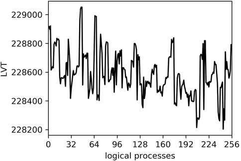
FIGURE 1. Snapshot of the LVT profile in the PCS model at GVT = 228124.556305. LVT and GVT are dimensionless quantities.

It is quite interesting that the analogy of the particular PDES algorithm, the conservative algorithm, with the KPZ model [14] can be used to classify possible PDES algorithms [13]. The reasoning is as follows: the KPZ equation is a partial differential equation. The solution to the partial differential equation is defined by the choice of specific boundary conditions. [13] expressed the idea that the type of synchronization of LPs with each other is associated with the boundary conditions of the PDES algorithms. Thus, the continuous boundary conditions correspond to the conservative scheme, the free boundary conditions correspond to the optimistic class of algorithms, and the fixed type of boundary conditions should correspond to the new class of PDES synchronization algorithms. This class is called the “freeze-and-shift” algorithm [13].

In the following subsections, we briefly describe two LVT profile simulation models that reflect the general features of conservative and optimistic algorithms and have similarities with the phase transitions in the KPZ model [14] and directed percolation model [16].

2.1 LVT in the conservative algorithm and KPZ equation

Korniss with co-authors noticed that the LVT profile evolution is similar to the process of surface growth [14]. They used an approach known as “simulation of simulation” to model the evolution of the LVT profile in conservative PDES. Specifically, they built a simulation model of LVT growth in a PDES simulation process. It is shown that the equation describing the random process of growth of local virtual time is a simplified form of the 1 + 1 KPZ equation, describing the growth of a one-dimensional profile in time. The KPZ universality class is characterized by three scaling exponents [15] that have the same values across a wide range of different models, including the LVT profile evolution model. This method allows us to use statistical physics tools to analyze parallel algorithms.

2.2 LVT in the optimistic algorithm and roughening transition

The above LVT evolution approach is adapted for optimistic PDES [16, 25]. The evolution of LVT in the optimistic synchronization scheme demonstrates features of the roughening transition universality class [18], to which the restricted solid-on-solid (RSOS) model, random deposition (RD) model, directed percolation (DP) model, and other statistical physics models belong [17].

There is a widespread opinion regarding the universality of growth models in the class of directed percolation [26], based on proposals formulated by Janssen [27] and [28]. According to these proposals, the model should belong to the DP universality class if the following four conditions are satisfied: 1) the model demonstrates a continuous phase transition from a roughening state into a unique stationary state; 2) the transition is characterized by a non-negative one-component order parameter; 3) the dynamic temporary rules are based only on short-range processes; and 4) the system does not have special attributes such as additional symmetry or quenched randomness.

In our case, all four conditions are fulfilled: 1) below the value of the parameter q_c, the average speed of the profile becomes equal to zero, and above this value q_c, the profile width increases; thus, the system demonstrates a roughening transition at a critical value q_c of the parameter q, defined in Eq. 2; 2) the order parameter is profile velocity, which is non-negative; 3) the rules of LP interactions are local; and 4) we have no quenched randomness and nothing special about the symmetry of the model. Therefore, we can expect that the LVT model will belong to the universality class of directed percolation.

2.3 LVT model and PDES analysis

LVT evolution models in PDES allow one to analyze the main fundamental properties of the PDES algorithm. For example, the zero speed of an LVT profile illustrates zero utilization time usage or possible deadlocks. Increasing profile width shows imperfect synchronization between LPs, which also reduces the simulation efficiency. The greater the LP LVT time difference, the more rollbacks can occur. A divergent LVT profile width may also indicate insufficient load balance (some LPs are ahead of others).

As mentioned above, the distinctive feature of the PDES model is similar to growing interface models in physics. Interestingly, a model with entirely different rules forms so-called universality classes, which are characterized by a set of universal critical exponents. These exponents describe the behavior of the model near the critical point. It can be assumed that most modifications to the Time Warp algorithm will not change the universal behavior of systems.

3 PCS network model

A two-dimensional mobile network, also known as a personal communication service (PCS) network, is a wireless communication network with distributed communication ports, each with its own coverage area or cell zone, set of communication channels, and users [19, 29, 30]. Users send and receive phone calls using these communication channels. When a user makes a phone call, the system tries to allocate a channel for the connection. If all channels are busy, the phone call terminates. The network is represented by square cells, assuming that each cell is assigned a fixed number of radio channels. The goal of PCS modeling is to minimize the probability of dropped calls.

The PCS model is implemented in the ROSS simulator [21]. ROSS serves as a simulation engine that provides a simulation loop for generating, dispatching, and processing events by parallel processes. It is implemented in the C++ programming language and uses the message-passing interface (MPI) for parallel operation. Parallel processes are optimistically synchronized.

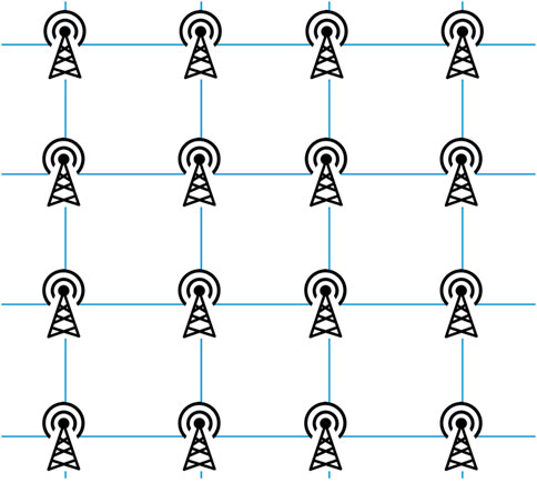
Let us describe the system in the language of logical processes and events. In this model, ports or cell zones are LP objects. LPs are located on a square lattice (Figure 2). The behavior of a phone call is modeled by different types of events. The system implements four different types of events: 1) NextCall—receipt of a call to a cell; 2) CompletionCall—completed cell call; 3) MoveOut—calling exit from the current cell (remote event); and 4) Moveln—indicates the arrival of a switching call in the cell.

FIGURE 2

FIGURE 2. Communication topology of the PCS network model.

In PCS, the time between events is distributed exponentially. The following parameters set the distribution means:

• MOVE_CALL_MEAN—average time between MoveOut events;

• NEXT_CALL_MEAN—average time between NextCall events;

• CALL_TIME_MEAN—average call duration.

Thus, a call can be scheduled to be sent to the current cell or to one of the neighboring cells. In the ROSS implementation, such events passing between LPs are called remote events. The proportion of deleted events is available in the output statistics. Let us denote this fraction as p. In other words, LPs are located on a square lattice with periodic boundary conditions, and the interaction between nearby LPs occurs with probability p. In addition to the number of remote events p, ROSS statistics provides data such as the total number of events processed, the number of events rolled back, and the rate of events. LVTs are available during the simulation.

3.1 Simulation of PCS

When modeling a PCS network, our primary focus is not on the likelihood of a phone going offline or other “physical” consequences. Instead, our analysis focuses on simulation performance as a function of simulation parameters. In the context of PDES, efficiency is typically measured in terms of event rate. This metric represents the number of events processed per unit of time. The frequency of events can be obtained from the output statistics of ROSS.

Furthermore, we monitor LVT throughout the simulation. From these data, we calculate two key metrics: the average speed of the LVT profile, as defined in Eq. 1, and the average width of the LVT profile, as defined in Eq. 3. These metrics provide valuable information about the performance and behavior of the simulated PCS network.

Average profile speed v(t):

$v\left(t\right)=\tau \left(t+1\right)-\tau \left(t\right),(1)$

where t is a GVT value when these data were collected and τ(t) is the LVT profile value averaged over N LPs, which is given as

$\tau \left(t\right)=\frac{1}{N}\sum _{i=1}^N{\tau }_i\left(t\right).$

Average profile squared width:

$w^2\left(t\right)=\frac{1}{N}\sum _{i=1}^N{\left[{\tau }_i\left(t\right)-\tau \left(t\right)\right]}^2.$

We would like to cover some technical details of the collection of ROSS statistics and other service calculations that are performed during the GVT calculation. GVT is calculated after processing a batch of events, which is determined by a model parameter. We set this parameter to 256 events per LP, which means the GVT is calculated when each LP has processed 256 events.

One of the main goals of the paper is to confirm the evolutionary model of the LVT. To achieve this, it is necessary to establish a connection between the parameters of the PCS model and LVT model.

In the context of the LVT evolution model [20], the key parameters are the fraction of remote events p and the growth rate q. In PCS, the main parameters are the means of distributions, including MOVE_CALL_MEAN, NEXT_CALL_MEAN, and CALL_TIME_MEAN. Among them, MOVE_CALL_MEAN is the only parameter that directly affects the number of remote events. Therefore, we have chosen MOVE_CALL_MEAN as the main parameter.

The analog of the parameter p in the PCS model may then be directly derived from the statistics as a percent of remote events. The growth rate q can be calculated using the following equation:

$q=1-\frac{\text{number\hspace{0.17em}of\hspace{0.17em}rollbacks}}{\text{number\hspace{0.17em}of\hspace{0.17em}all\hspace{0.17em}processed\hspace{0.17em}events}},(2)$

where the number of rollbacks and the total number of processed events are available from the statistics.

To simulate the PCS network model, we use the ROSS simulation engine on two compute nodes, each equipped with two Intel(R) Xeon Platinum 8164 2.0 GHz processors and 2 × 768 GB of on-chip DDR4 2666 MHz memory. The number of LPs is set to 64, 144, or 256. The MOVE_CALL_MEAN (MCM) parameter ranges from 50 to 100000. For each MCM value, we record the corresponding p and q values and then calculate their averages for 10 independent runs (for example, see Table 1). Figure 3 illustrates how the growth rate of q varies with the ratio p of remote events. The lower the number of interprocess communications, the lower the number of rollbacks, and consequently, the higher the growth rate. These averaged values of p and q are subsequently used as parameters of the LVT model.

TABLE 1

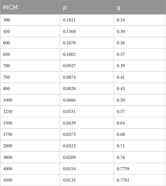
TABLE 1. Correspondence between MCM and the values of p and q for the number of nodes N = 256 in the PCS model.

FIGURE 3

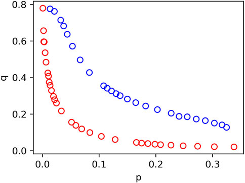
FIGURE 3. Correlation between parameters p and q. Blue dots show data from Table 1 for the number of nodes N = 256, and red dots correspond to N = 64.

4 LVT-PCS model

Let us construct a model of the evolution of the LVT in the described PCS model, the LVT-PCS model. An important difference between the LVT–PCS model and the general optimistic LVT model [25] is that the parameters p and q are now interdependent and cannot be chosen independently. However, we expect that in the vicinity of the roughening transition, the behavior of the LVT–PCS model will be essentially similar to that of the general LVT model and belong to the DP universality class.

In the LVT–PCS profile evolution model, we, as usual, use the assumption that events are Poisson arrivals, so the time between them is exponentially distributed. Simulation parameters are

• N—total number of LPs,

• T—total number of time steps,

• q—growth rate,

• p—probability of remote events.

The values of q and p are set equal to the values of q and p, obtained from the PCS simulation on ROSS.

We first create the LP topology. Since the LPs in ROSS are implemented on a two-dimensional square lattice, in LVT–PCS, we also place the LPs on a two-dimensional square lattice (Figure 2). Each LP can exchange messages with its four nearest neighbors.

The simulation starts with a flat profile τ_i = 0 and i = 0. N − 1, where τ_i is the local virtual time of the ith LP. Next, at each modeling step t, the free growth of the profile is first simulated, and then, rollbacks are simulated.

Modeling free growth means increasing the LVT of each LP by an exponentially distributed random variable η_i with the unit mean:

${\tau }_i\left(t+1\right)={\tau }_i\left(t\right)+{\eta }_i,i=1,\dots ,N.$

At this optimistic stage, we model the profile growth, assuming that no violation of the causality has occurred. After this step, we simulate rollbacks. The total number of LPs that need to rollback their LVTs is regulated by the growth rate parameter q (see Eq. 2). Let us denote the average number of rolled back LPs as bN. Assuming that all N LPs proceed at the first step and bN LPs rollback on average, from Eq. 2, we have

$q=1-\frac{bN}{N+bN}=\frac{1}{1+b}.(3)$

From Eq. 3, we obtain

$b=\frac{1}{q}-1.$

Therefore, to simulate rollbacks, we randomly select, on average, bN LPs, which local time will rollback. If the LVT of LP is greater than that of one of its neighbors, chosen with probability p, then the LVT is reduced to the neighbor’s time.

After each time step t, we calculate the average profile velocity v(t) (1) and the average profile width w²(t) (3). In computer science parlance, the average speed of a profile v is related to the efficiency of the simulation, which is the average load of the parallel processes. In addition, the average profile width w² is associated with desynchronization between processing elements. The larger the profile width, the more desynchronized the simulation.

The final results are calculated as the average of R independent runs of the random process:

$⟨\tau \left(t\right)⟩=\frac{\sum _R\tau \left(t\right)}{R},$

$⟨v\left(t\right)⟩=\frac{\sum _{R}v\left(t\right)}{R},$

$⟨w^2\left(t\right)⟩=\frac{\sum _R{w}^2\left(t\right)}{R}.$

4.1 Common simulation protocol for PCS and LVT–PCS models

The dependent modeling procedure for the PCS and LVT–PCS models is as follows:

1. Simulate the PCS network model with the MOVE_CALL_MEAN parameter chosen from the range [50, 100000].

2. Monitor LVT during simulation.

3. Save the corresponding values of q and p.

4. Simulate the LVT–PCS model with the same values of p and q.

5 Data analysis

The main result of our simulation is that the behavior of the LVT profiles in both models is qualitatively similar near the roughening transition q_c. Near the transition, there are more remote events, and the LVT growth speed becomes lower, as does the event rate (i.e., efficiency), and the average profile width stops growing [31, 20] (i.e., synchronization becomes better), and at the transition value q_c, there is a deadlock in the PCS model.

A comparison of the average profile velocity in the LVT–PCS and PCS models and the event rate in the PCS model is presented in Figures 4, 5. The average velocity in the LVT model corresponds to event utilization in the PCS models (i.e., event rate).

FIGURE 4

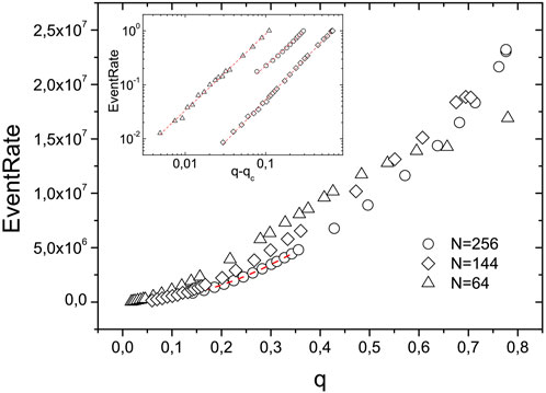
FIGURE 4. Event rate in the PCS model as a function of rollback frequency for N = 64, 144, and 256. Error bars are smaller than symbols. Inset: critical behavior of the event rate depending on the reduced parameter q − q_c.

FIGURE 5

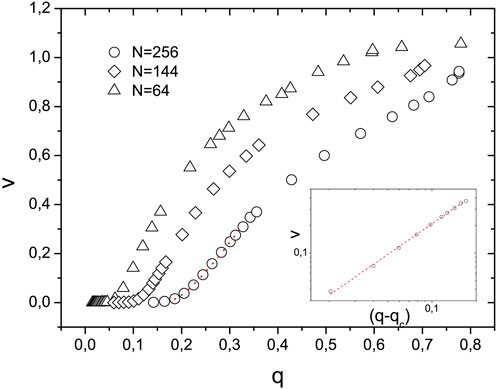
FIGURE 5. Average LVT velocity in the LVT–PCS model as a function of q for N = 64, 144, and 256. Error bars are smaller than symbols. Inset: critical behavior of the LVT velocity depending on the reduced parameter q − q_c.

The dependence of the event rate ER on the value of the parameter q is shown in Figure 4. It can be seen that the symbols calculated for system sizes N = 64, 144, and 256 approach each other at a low event rate. We approximate the event rate data using the expression $ER=E{R}_0{(q-q_c)}^{\nu }+\text{const}$ and estimated values q_c = 0.064 and ν = 1.345(9) in the case of the largest system size N = 256. Fitting smaller values of N is unreliable as it is well-known that for small system values, scaling corrections can be large [32]. The value ν ≈ 1.3 [17] apparently corresponds to the DP 2 + 1 universality class. The value q_c is a deadlock critical value, i.e., deadlocks occur at point q = q_c, and the profile speed becomes zero. The conditions mentioned at the end of Section 2.2 are satisfied—there is a roughening transition at q = q_c, the event rate is non-negative, the rules are local, and there is no quenched randomness. To summarize, we can conclude that the behavior of the PCS model near the deadlock value belongs to the DP 2 + 1 universality class.

We use the p and q values estimated in the PCS model to simulate the LVT–PVS model. Figure 5 shows the resulting dependence of the average profile velocity in the LVT–PCS model on the parameter q. There are three ranges of q with different velocity dependences. First, for the case of N = 256, this is zero velocity below the value q_c = 0.185(1), which is the roughening critical point [18]. Second, we use the profile approximation $v=v_0{(q-q_c)}^{\nu }+\text{const}$ of the data in the range q_c < q < 0.3. We estimate the value of the exponent ν = 1.3(1), which is close to the value ν_DP of the directed percolation model in the 2 + 1 dimension, ν_DP ≈ 1.3 [18, 17]. Third, it is a random deposition mode, with a value close to 0.8, where the profile grows randomly on each LP and the average speed reaches a value of unity, the maximum possible profile speed.

Finite-size effects are visible in Figure 5 as a shift in the position q* of velocity that vanishes with the size of the system. General theory (for example, see [32]) predicts that the value of the parameter q* depends on the size of the system and scales with some exponent. We cannot correctly estimate q*(N) for systems of sizes 64 and 144 and provide only a qualitative explanation of the shift. The LVT–PCS model captures important properties of the PCS model that were not known prior to our analysis, exploiting the profile’s similarity to those of the statistical physics of surface growth.

Figure 6 shows the growth of the squared profile width in the LVT–PCS model for two system sizes N = 64 and 256 and for several values of parameter pairs (q, p). For values of q below the corresponding value of q*(N), the width does not increase after some time of transition to the absorbing state. At large values of q, saturation occurs as a function of the values of (q, p), and before this, the system has a value of the exponent β close to 1/2. We summarize estimates of the effective exponent β in Figure 7, which shows a smooth change in 2β, as q increases. This is another illustration of the cross-over from the DP fixed point to the random deposition fixed point.

FIGURE 6

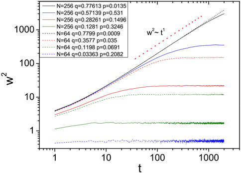
FIGURE 6. Average profile width in the LVT–PCS model as a function of simulation time. The width increases as w² ∼ t^2β.

FIGURE 7

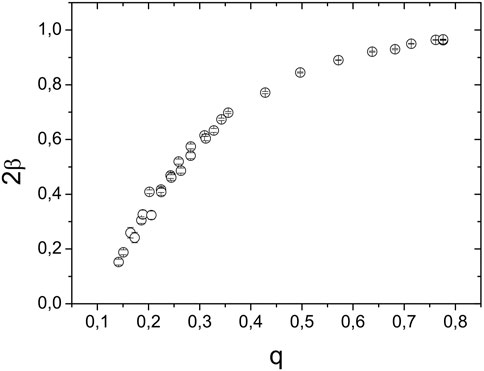
FIGURE 7. Value of 2β depending on the parameters p and q in the LVT–PCS model for system size N = 256.

6 Summary and discussion

In this study, we applied the previously proposed optimistic LVT evolution model [16, 20] to analyze the simplest mobile network model, the portable communication service (PCS) model. We propose a way to relate the parameters of the PCS model and our LVT model. We call the resulting model the LVT–PCS model, emphasizing the fact that it uses parameter values specific to the PCS model. This is a way to model the specific behavior of a PDES model using the LVT growth model.

We first simulate the PCS model using the ROSS simulator [21] and extract the values of q and p. Next, we use q and p as input parameters when simulating the LVT–PCS model. In the LVT–PCS model, the parameter q is related to the number of rollbacks in the optimistic algorithm and the parameter p is the probability of time synchronization with one of the cell neighbors. By matching the parameters, our model was used to analyze deadlocks and synchronizations in the PCS model.

We found a roughening transition at q_c in the LVT–PCS model, which apparently belongs to the directed percolation universality class of [17, 26] in dimension 2 + 1. This corresponds to a deadlock in the PCS model. For values of q > q_c, the velocity profile behaves as a power of q with an exponent close to 1.3, which is an estimate of the correlation length exponent in the DP 2 + 1 universality class. Thus, we know how the event rate behaves in the PCS model near the deadlock. An increase in the width of the LVT profile w was observed over time, with an exponent also corresponding to the DP 2 + 1 universality class.

There is a second extremum with a value of q close to unity, which corresponds to the universality class of random ballistic deposition. Again, the behavior of the PCS and LVT–PVS models is similar at this limit.

Between these two extremes, one should not expect universal behavior since it represents a transition from one fixed point of the DP universality class at q = q_c to a second fixed point of the ballistic deposition universality class at q = 1. The crossover region is known to reflect specific details of the models, and it is not surprising that slightly different behavior is observed in the intermediate q region at approximately 0.5.

We hope that the proposed approach can be generalized and applied to other optimistic PDES models. Future research may consider extending this approach to other models and assessing its effectiveness. Additionally, it would be useful to study the practical implications of this approach, such as its potential to improve system performance, reduce resource usage, and improve scalability. These results may have important implications for the computational community and ultimately lead to more efficient and effective modeling methods.

The work was carried out at the Institute of Solid State Physics of the Russian Academy of Sciences within the framework of the state assignment of the Russian Ministry of Education and Science.

Data availability statement

The original contributions presented in the study are included in the article/Supplementary material; further inquiries can be directed to the corresponding author.

Author contributions

All authors listed have made a substantial, direct, and intellectual contribution to the work and approved it for publication.

Conflict of interest

The authors declare that the research was conducted in the absence of any commercial or financial relationships that could be construed as a potential conflict of interest.

Publisher’s note

All claims expressed in this article are solely those of the authors and do not necessarily represent those of their affiliated organizations, or those of the publisher, the editors, and the reviewers. Any product that may be evaluated in this article, or claim that may be made by its manufacturer, is not guaranteed or endorsed by the publisher.

References

1. Barnes P. Challenges in simulating communication systems: state of the art and open challenges in simulating network and communications systems. Proc 2022 ACM SIGSIM Conf Principles Adv Discrete Simulation (2022) 118–25. doi:10.1145/3518997.3534120

CrossRef Full Text | Google Scholar

2. Kim YJ, Mavris D, Fujimoto R. Time-and space-parallel simulation of air traffic networks. Simulation (2019) 95:1213–28. doi:10.1177/0037549719831358

CrossRef Full Text | Google Scholar

3. Andelfinger P, Piccione A, Pellegrini A, Uhrmacher A. Comparing speculative synchronization algorithms for continuous-time agent-based simulations. In: 2022 IEEE/ACM 26th International Symposium on Distributed Simulation and Real Time Applications (DS-RT); 26-28 September 2022; Alès, France. IEEE (2022). p. 57–66.

CrossRef Full Text | Google Scholar

4. Plimpton S, Thompson A, Slepoy A. Stochastic parallel particle kinetic simulator. Tech. rep. Albuquerque, NM (United States): Sandia National Lab.(SNL-NM) (2008).

Google Scholar

5. Savva GD, Benson RL, Christidi I-A, Stamatakis M. Exact distributed kinetic Monte Carlo simulations for on-lattice chemical kinetics: lessons learnt from medium-and large-scale benchmarks. Philosophical Trans R Soc A (2023) 381:20220235. doi:10.1098/rsta.2022.0235

CrossRef Full Text | Google Scholar

6. Rodgers TM, Mitchell JA, Tikare V. A Monte Carlo model for 3d grain evolution during welding. Model Simulation Mater Sci Eng (2017) 25:064006. doi:10.1088/1361-651x/aa7f20

CrossRef Full Text | Google Scholar

7. Steinman JS (1992). Speedes - a multiple-synchronization environment for parallel discrete-event simulation.

Google Scholar

8. Qu Q, Yao Y, Tang W, Zhu F. Research on simulation communication mechanism for intelligent combat. In: 2022 IEEE 2nd International Conference on Electronic Technology, Communication and Information (ICETCI); 27-29 May 2022; Changchun, China. IEEE (2022). p. 1456–9.

CrossRef Full Text | Google Scholar

9. Fujimoto RM. Parallel discrete event simulation. Commun ACM (1990) 33:30–53. doi:10.1145/84537.84545

CrossRef Full Text | Google Scholar

10. Bryant RE. Simulation of packet communication architecture computer systems. Massachusetts Institute of Technology (1977).

Google Scholar

11. Chandy KM, Misra J. Distributed simulation: a case study in design and verification of distributed programs. IEEE Trans Softw Eng (1979) 440–52. doi:10.1109/tse.1979.230182

CrossRef Full Text | Google Scholar

12. Jefferson DR. Virtual time. ACM Trans Programming Languages Syst (Toplas) (1985) 7:404–25. doi:10.1145/3916.3988

CrossRef Full Text | Google Scholar

13. Shchur LN, Novotny MA. Evolution of time horizons in parallel and grid simulations. Phys Rev E (2004) 70:026703. doi:10.1103/physreve.70.026703

PubMed Abstract | CrossRef Full Text | Google Scholar

14. Korniss G, Toroczkai Z, Novotny MA, Rikvold PA. From massively parallel algorithms and fluctuating time horizons to nonequilibrium surface growth. Phys Rev Lett (2000) 84:1351–4. doi:10.1103/physrevlett.84.1351

PubMed Abstract | CrossRef Full Text | Google Scholar

15. Kardar M, Parisi G, Zhang Y-C. Dynamic scaling of growing interfaces. Phys Rev Lett (1986) 56:889–92. doi:10.1103/physrevlett.56.889

PubMed Abstract | CrossRef Full Text | Google Scholar

16. Ziganurova L, Novotny M, Shchur L. Model for the evolution of the time profile in optimistic parallel discrete event simulations. J Phys Conf Ser (IOP Publishing) (2016) 681:012047. doi:10.1088/1742-6596/681/1/012047

CrossRef Full Text | Google Scholar

17. Ódor G. Universality classes in nonequilibrium lattice systems. Rev Mod Phys (2004) 76:663–724. doi:10.1103/revmodphys.76.663

CrossRef Full Text | Google Scholar

18. Alon U, Evans M, Hinrichsen H, Mukamel D. Roughening transition in a one-dimensional growth process. Phys Rev Lett (1996) 76:2746–9. doi:10.1103/physrevlett.76.2746

PubMed Abstract | CrossRef Full Text | Google Scholar

19. Carothers CD, Fujimoto RM, Lin Y-B, England P. Distributed simulation of large-scale pcs networks. In: Proceedings of International Workshop on Modeling, Analysis and Simulation of Computer and Telecommunication Systems; 31 January 1994 - 02; Durham, NC, USA. IEEE (1994). p. 2–6.

Google Scholar

20. Ziganurova L, Shchur LN. Synchronization of conservative parallel discrete event simulations on a small-world network. Phys Rev E (2018) 98:022218. doi:10.1103/physreve.98.022218

PubMed Abstract | CrossRef Full Text | Google Scholar

21. Carothers CD, Bauer D, Pearce S. Ross: a high-performance, low-memory, modular time warp system. J Parallel Distributed Comput (2002) 62:1648–69. doi:10.1016/s0743-7315(02)00004-7

CrossRef Full Text | Google Scholar

22. Lubachevsky BD. Efficient parallel simulations of dynamic ising spin systems. J Comput Phys (1988) 75:103–22. doi:10.1016/0021-9991(88)90101-5

CrossRef Full Text | Google Scholar

23. Metropolis N, Rosenbluth AW, Rosenbluth MN, Teller AH, Teller E. Equation of state calculations by fast computing machines. J Chem Phys (1953) 21:1087–92. doi:10.1063/1.1699114

CrossRef Full Text | Google Scholar

24. Lamport L. Time, clocks, and the ordering of events in a distributed system. Commun ACM (1978) 21:558–65. doi:10.1145/359545.359563

CrossRef Full Text | Google Scholar

25. Shchur L, Ziganurova L. Synchronization of processes in parallel discrete event simulation. J Exp Theor Phys (2019) 129:722–32. doi:10.1134/s106377611910025x

CrossRef Full Text | Google Scholar

26. Hinrichsen H. Non-equilibrium critical phenomena and phase transitions into absorbing states. Adv Phys (2000) 49:815–958. doi:10.1080/00018730050198152

CrossRef Full Text | Google Scholar

27. Janssen H-K. On the nonequilibrium phase transition in reaction-diffusion systems with an absorbing stationary state. Z für Physik B Condensed Matter (1981) 42:151–4. doi:10.1007/bf01319549

CrossRef Full Text | Google Scholar

28. Grassberger P (1982). On phase transitions in schlögl’s second model. Z für Physik B Condensed Matter. 47. 365–74. doi:10.1007/978-3-642-81778-6_49

CrossRef Full Text | Google Scholar

29. Lin Y-B, Fishwick PA. Asynchronous parallel discrete event simulation. IEEE Trans Syst Man, Cybernetics-A: Syst Humans (1996) 26:397–412. doi:10.1109/3468.508819

CrossRef Full Text | Google Scholar

30. Carothers CD, Fujimoto RM, Lin Y-B. A case study in simulating pcs networks using time warp. ACM SIGSIM Simulation Dig (1995) 25:87–94. doi:10.1145/214283.214309

CrossRef Full Text | Google Scholar

31. Korniss G, Novotny MA, Guclu H, Toroczkai Z, Rikvold PA. Suppressing roughness of virtual times in parallel discrete-event simulations. Science (2003) 299:677–9. doi:10.1126/science.1079382

PubMed Abstract | CrossRef Full Text | Google Scholar

32. Landau DP, Binder K. A guide to Monte Carlo simulations in statistical physics. 4 edn. Cambridge University Press (2014). doi:10.1017/CBO9781139696463

CrossRef Full Text | Google Scholar