
94% of researchers rate our articles as excellent or good
Learn more about the work of our research integrity team to safeguard the quality of each article we publish.
Find out more
ORIGINAL RESEARCH article
Front. Phys., 08 January 2024
Sec. Medical Physics and Imaging
Volume 11 - 2023 | https://doi.org/10.3389/fphy.2023.1335285
This article is part of the Research TopicAdvances of Synchrotron Radiation-Based X-Ray Imaging in Biomedical ResearchView all 6 articles
 Ju Young Lee1,2*
 Sandro Donato3,4
 Andreas F. Mack5
 Ulrich Mattheus5
 Giuliana Tromba6
 Elena Longo6
 Lorenzo D’Amico6,7Sebastian Mueller2Thomas Shiozawa5Jonas Bause2Klaus Scheffler2,8
 Renata Longo7,9†
 Gisela E. Hagberg2,8†
X-ray phase-contrast micro computed tomography using synchrotron radiation (SR PhC-µCT) offers unique 3D imaging capabilities for visualizing microstructure of the human brain. Its applicability for unstained soft tissue is an area of active research. Acquiring images from a tissue block without needing to section it into thin slices, as required in routine histology, allows for investigating the microstructure in its natural 3D space. This paper presents a detailed step-by-step guideline for imaging unstained human brain tissue at resolutions of a few micrometers with SR PhC-µCT implemented at SYRMEP, the hard X-ray imaging beamline of Elettra, the Italian synchrotron facility. We present examples of how blood vessels and neurons appear in the images acquired with isotropic 5 μm and 1 µm voxel sizes. Furthermore, the proposed protocol can be used to investigate important biological substrates such as neuromelanin or corpora amylacea. Their spatial distribution can be studied using specifically tailored segmentation tools that are validated by classical histology methods. In conclusion, SR PhC-µCT using the proposed protocols, including data acquisition and image processing, offers viable means of obtaining information about the anatomy of the human brain at the cellular level in 3D.
There is a great interest in studying the three-dimensional microstructure of human tissues, which is critical for improving our understanding of the spatial relationship between anatomical structures. Classical histology is the analysis of thin tissue slices that are stained and imaged using optical microscopyThis is the gold standard for many biological fields, such as neuroscience. However, histology presents some disadvantages: during the sectioning deformations are introduced and it provides only 2D information. Advancement in image processing allows for correction of non-linear deformations to reconstruct 3D volumes [1–3]. However, the histology slices are sometimes torn or folded, introducing discontinuities that may limit 3D reconstruction.
Ideally, tissue microstructure information could be obtained directly in 3D space. Light-sheet imaging is emerging as a sensitive and specific tool for volumetric imaging. However, the process of tissue clearing and labeling is required prior to imaging [4]. Application of this technique can be challenging for large human samples [5]. While magnetic resonance imaging (MRI) and computed tomography (CT) are valuable sources for internal structure of the brain in clinical settings, they are limited in spatial resolution and image contrast.
In ex vivo MRI, where tissues are taken out of the body, the spatial resolution can be improved. In fact, ex vivo MRI of whole brain has been acquired with minimum voxel sizes of 1003–4003 μm3 [6,7]. For smaller samples, smaller voxel can be achieved within feasible measurement time with high field scanners. For instance, 373 μm3 voxel size for samples with a diameter of 4 cm has been demonstrated [8]. Recent developments of dedicated hardware open up the prospect to perform MRI at the cellular level [9,10], albeit within a limited total spatial coverage of a few hundred micrometers. However, the magnetic properties of the tissue, which is reflected in MRI contrast, are influenced by the fixation procedure and the embedding media which limits reproducibility across tissue preparation pipelines [11–13].
The image contrast in CT arises from the attenuation of X-ray beams as they pass through different materials. The attenuation depends on the material composition and the density. In soft tissue, there are no large differences between biological compartments, resulting in weak–or nearly absent-intrinsic contrast. Therefore, prior to CT imaging, the samples are usually injected with exogenous contrast agents that have densities higher than soft tissue. For example, in order to investigate the blood vessel structure, perfusion of contrast agents such as Microfil or Indian Ink into the blood vessels can be performed [14,15]. Using conventional clinically available CT systems, typical voxel-sizes are 4003–6003 μm3, while the addition of photon-counting can push this value to 1503 μm3 [16].
Coherent X-rays can also yield contrast dependent on subtle phase shifts occurring in the tissue. Among such phase-sensitive techniques, propagation-based imaging (PBI), sometimes called free-space-propagation or single distance imaging, is available at several synchrotron light sources [17]. These allow detection of subtle phase shifts that arise when X-rays through materials with varying refractive indices and can be interpreted as a local deformation of the X-ray wavefront. The phase difference between two X-rays passing at the interface between two compartments with different refractive indices, results in an interference pattern. This further develops as the beam propagates along an extended pathway free of obstacles.
In PBI, the sample-to-detector distance must be sufficient to allow the effects of subtle phase shifts caused by small structures to play out and be detected. The resulting image shows a sharp fringe edge enhancement at the tissue interfaces which is proportional to the Laplacian of the phase-shift [18]. Through the application of a phase-retrieval algorithm, the fringes are compensated, and the original edge-enhanced image becomes an area contrast image. In case of small differences between the refractive indices, which is plausible in unstained tissue scanned in the near-field regime, the Paganin’s phase-retrieval algorithm can be employed [19]. Since the algorithm acts as a low pass filter, the final image has a higher signal-to-noise ratio than an attenuation image acquired without any free-space propagation would have. It is worth of notice that the phase-retrieval algorithm decreases the noise level of the image without affecting the spatial resolution [20].
SR PhC-µCT images allow mapping the underlying anatomical structures, with high contrast-to-noise ratio despite the absence of large differences in electron density within the tissue. Hence, SR PhC-µCT is regarded as a suitable tool for virtual histology [21–23]. Although it can be combined with injected contrast agents, these are not necessary per se to achieve high tissue contrasts. A wide palette of tissue preparations, like formalin- ethanol- or xylene-soaked tissue as well as paraffin embedded samples can be used for imaging with SR PhC-µCT [24]. Imaging of unstained paraffin embedded samples are of particular importance, since this type of samples are common in many brain banks.
Several studies have used SR PhC-µCT to investigate the microstructure of unstained human organs [25–27]. Some have acquired images from human brain samples with sub-cellular detail and successfully segmented neurons to study their three-dimensional spatial distributions [28,29]. SR PhC-µCT also has the potential for detecting pathology such as amyloid plaques and mineralized blood vessels [30,31].
With experience of several beamtime sessions at the SYRMEP beamline of Elettra synchrotron, we have developed a pipeline that works reliably with unstained human brain tissue (Figure 1). We present a step-by-step guideline with emphasis on important decisions that need to be made at each step. We also describe how segmentation tools can be tailored to identify specific structures, and how these can be directly validated by classical histology methods applied to the same specimens. Segmentation methods were developed to identify blood vessels as well important biological substrates such as neuromelanin or corpora amylacea. Although the suggestions presented here are mainly relevant for the SYRMEP beamline, some of our proposed methods may be useful for SR PBI micro-CT performed at other synchrotron facilities. For example, we explored the transferability of some of our segmentation method to images obtained at other beamlines.

FIGURE 1. Complete workflow for the virtual histology of human brain tissue. (A) First, the target brain region is cut out and immersed in a fixative agent. The presented picture shows the cortical areas surrounding the central sulcus, which includes the primary motor and somatosensory regions. (B) If applicable, structural MRI may be acquired. (C) The tissue is cut into 1 cm thick sections to fit into the embedding cassettes. The left tissue is the hand area of the primary motor cortex and the right tissue is the hand area of the somatosensory cortex. (D) The tissues are embedded in paraffin and (E) brought to the biomedical imaging beamline of a synchrotron facility (F) After the beamtime, the paraffin blocks are sectioned into thin slices for (G) microscopy scanning. (Image credits for (E) is EPSIM 3D/JF Santarelli, Synchrotron Soleil).
The first step is to obtain ex vivo tissue. We obtained tissue from Tübingen University body donor program at the Institute of Clinical Anatomy and Cell Analysis. The body donors provided informed consent, in alignment with the Declaration of Helsinki’s guidelines for research, to donate their bodies for research purposes. The ethics commission at the Medical Department of the University of Tübingen approved the research procedure. It is also possible to obtain samples from brain banks that are already fixed and embedded (e.g., Netherlands brain bank).
Brain regions like the choroid plexus and pineal gland are likely to be calcified in aged subjects [32,33]. Provided their anatomical locations are known, these areas should be cut out to minimize the risk of artifacts. For the X-ray energy spectrum optimal for soft tissue contrast, the presence of significant calcium content leads to pronounced streaking artifacts due to its higher absorption compared to the surrounding tissues [34]. An example of such effects caused by calcifications in the pineal gland is shown in Supplementary Figure S1.
After dissecting the targeted region, the tissues are either perfusion or immersion fixed using a fixative agent, for instance ethanol or perhaps more typically a formalin solution containing 4% formaldehyde. Fixation time depends on the size of the sample. In case of human brain stems, we kept them in fixative solution for a minimum of 3 weeks, based on the experimentally determined diffusion-coefficient of the used fixative. If available, magnetic resonance imaging (MRI) can be scanned at this stage. In our case, we used a formalin solution that is optimized for ev vivo MRI at high magnetic field strengths [13]. Quantitative MRI can be used to check the advancement of the fixation process. Moreover, MRI is useful for calculating the shrinkage ratio introduced by paraffin embedding, which is the next step [13,27,35,36].
The choice of the fixative agent will impact the tissue shrinkage ratio [24,37] and tissue contrast in the resulting image [38]. For example, the fiber tract contrast is improved when tissue is fixed with 100% ethanol compared to formalin [24].
Different embedding materials may be used in accordance with the research scope [38]. We used formalin-fixed paraffin-embedding (FFPE) which is suitable for histology afterwards. Many researchers have used cylindrically shaped biopsy punches with diameter and height of a few millimeters [28,31,32]. In contrast, we used larger samples than usual size for routine histology, with width and height of 2–3 cm. Therefore, extra care was taken during the paraffin embedding process. The automated embedding station normally employed for smaller samples may lead to incomplete paraffin penetration and large deformation such as dented surfaces (Supplementary Figure S2) [40].
In order to reduce SR PhC-µCT image artifacts, we advise to prevent air bubbles from being trapped in the paraffin blocks. Air-tissue boundaries create strong edge-enhancements that will turn into strong image artifacts due to large difference in their refractive indices (Supplementary Figure S1). In order to minimize the occurrence of entrapped air bubbles, we placed the sample in vacuum during the paraffin embedding process. The use of vacuum pumping during the embedding process is a routine practice in resin embedding for electron microscopy and is therefore known not to damage the tissue. Some residual air bubbles may remain even with repeated degassing processes [41]. Other approaches such as keeping the paraffin wax at 60° for a long time could be considered to further improve this process [40].
Elettra is a third-generation synchrotron located in Trieste, Italy. It is equipped with 263 m long electron storage ring that supplies several beamlines, including SYRMEP (SYnchrotron Radiation for MEdical Physics) beamline. The beamline bending magnet provides polychromatic light in the energy range from ∼8.5–40 keV. The X-ray source is located at > 20 m from the experimental station, thus the impinging beam has high spatial coherency, allowing for propagation-based phase-contrast imaging. In our experiment, the polychromatic (white) beam mode, rather than monochromatic beam mode, was used to maximize the photon flux. With a silicon filter, the average energy of the beam was 20 keV [42].
Inside the experimental station of the SYRMEP beamline, the sample is placed on a rotating stage at a 23 m distance from the light source (Figure 2). The beam height at this position is approximately 4 mm. Even if a larger footprint of the beam can be used for image acquisition, our recommendation is to limit the beam size to the full-width-half-maximum. It will allow to obtain a more homogeneous signal-to-noise ratio within images of the same dataset. Acquisitions were performed with a 2048 × 2048 sCMOS detector with a physical pixel size of 6.5 μm. The used detector was coupled with a high-numerical aperture optic allowing to select effective pixel sizes between 0.9 um and 5 um. The X-ray was converted into visible light through a gadolinium gallium garnet Eu-doped (GGG:Eu) scintillator screen [43]. The pixel size determines the vertical field-of-view (FOV). If the height of the sample is bigger than the beam height as shown in Figure 2, the entire vertical length cane be covered by multiple tomographic acquisitions (further elaborated in Step 2d).
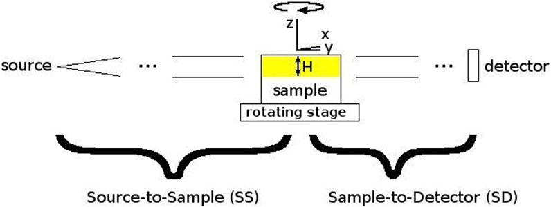
FIGURE 2. Schematic picture of the beamline setup. To obtain tomographic reconstructions, the sample is rotated around the vertical Z-axis. H is the source height.
In practice, we opted for two beamline setups. One encompassing larger pixels of ∼5 μm × 5 µm to increase the FOV of each acquired image, another with smaller pixels of ∼1 μm × 1 µm to allow observations of finer details (Figure 3, Table 1). Since the phase-shift pattern depends on the sample-to-detector distance, this parameter has to be optimized according to the detector pixel size. Below, we explain additional factors to consider during the beamtime in detail.
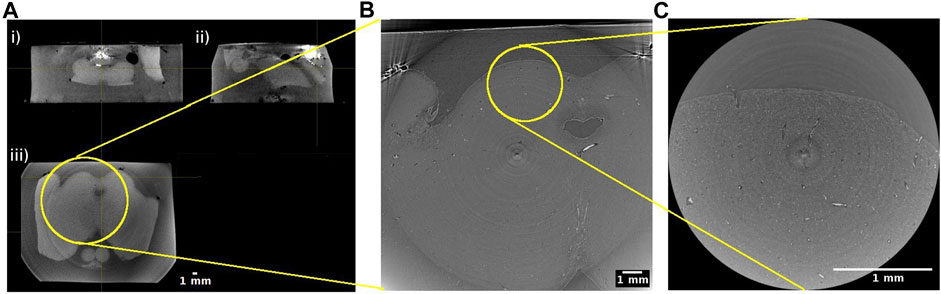
FIGURE 3. Hierarchical imaging of the midbrain of the human brainstem. (A) Cone beam imaging from Tomolab (Elettra, Trieste) covers the entire volume of the sample and is acquired with a voxel size of 20 µm. Orthogonal views showing i) coronal; ii) sagittal; and iii) axial views through the sample. Axial views from synchrotron radiation phase-contrast microtomography acquired with 5 µm isotropic voxel (B) and 1 µm isotropic voxel (C). Yellow circles indicate the matching regions when going from the lower to the higher resolution measurements.
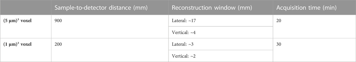
TABLE 1. Hierarchical imaging beamline setup for propagation-based phase-contrast microtomography. The specifications apply to experiments at SYRMEP beamline at Elettra synchrotron facility. The details may vary between sites.
We utilized the PBI, which is applicable in the near-field region. This condition is met for large Fresnel numbers NF = deff2/(λReff) >> 1, where deff is the effective pixel size, Reff is the sample-to-detector distance multiplied with the square of the magnification factor (the ratio of the source to detector over the source to sample distance) and λ is the X-ray wavelength. In experimental practice, this condition is often relaxed to allow NF to be closer to 1. Once the detector pixel size is determined, this condition places a constraint on the maximum propagation distance. In the context of FFPE human tissues, the signal-to-noise ratio in reconstructed images is optimized for NF > 2 [43].
In our measurements, a sample-to-detector distance of 90 cm was used for the ∼5 µm pixel size and 20 cm was used for the ∼ 1 µm pixel size. In future studies, these distances can be optimized in order to obtain better signal-to-noise ratio [43].
When imaging a large sample like parts of the human brain, it is strongly recommended to acquire data using at least two pixel size settings. Images with a larger pixel size will have a larger field of view, covering several landmarks of the sample. Images with a smaller pixel size will be a zoomed in image with a smaller field of view. This method is sometimes referred to as hierarchical imaging or multi-scale imaging [25]. Even if the research question only concerns the microstructure of a particular part of the tissue, it is always advisable to acquire images with a larger field of view as a reference. Otherwise, it may be challenging to infer the exact location of the high spatial resolution image and to position the acquired information within its exact anatomical context (Figure 3).
High resolution detectors for soft tissue CT are usually indirect conversion type, requiring incident X-ray beam to be converted into visible light. Typically, a scintillator screen is used for converting the beam. Synchrotron beamlines commonly employ optical systems that allow for selecting different scintillator types [44]. When selecting a scintillator, users need to consider the conversion efficiency of the X-rays to visible light and its impact on spatial resolution. Thicker scintillators exhibit higher efficiency, but may also increase signal blurring, consequently reducing spatial resolution. On the other hand, thinner scintillation materials better preserve spatial resolution but have lower efficiency, requiring longer exposure times. Balancing between acquisition time and the desired resolution is essential. At SYRMEP beamline, we used GGG:Eu scintillators with thickness of 45 µm for a voxel size of 53 μm3 and 17 µm thickness for a voxel size of 13 μm3 (Supplementary Figure S3).
Based on the decided pixel size, it is possible to estimate the size of the FOV. Typically, the considered reconstruction window will have sizes determined by the width of the photon detector. In order to enlarge the horizontal FOV, the rotation axis can be placed off-center, i.e., at one edge of the camera FOV. This approach is known as extended FOV (or half-acquisition) method [45]. This method requires a dedicated pre-processing, called stitching of the sinogram prior to reconstruction which is explained in Step 3a.
If the extended FOV is smaller than the brain sample under investigation, it is helpful to plan ahead how to position the FOV of each acquisition. We cut out circular shapes from an adhesive tape with diameter corresponding to the size of the FOV. The circular shape corresponds to an area that excludes the four corners of the acquired image with low sampling density. For the acquisitions with voxel sizes of 53 μm3, the diameter was about 1.7 cm. These circles were placed on top of the specimen to mark each FOV. The number of circles required then gave information about how many scans were needed to obtain full coverage the region of interest, also known as mosaic CT. As a reference to position the sample, a marker is placed above the center of each FOV for ‘Step 2f’ (Figure 4).
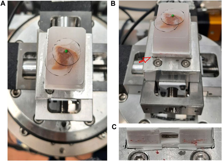
FIGURE 4. Sample positioning and coverage planning at SYRMEP beamline experimental station (A) A paraffin embedded brain sample was placed on the rotator. The coverage of the measurement was estimated by a transparent plastic film placed on the sample surface. A small green polymer clay, which serves as a radiopaque marker, was placed in the center. (B) The same setting as panel A with picture taken from slightly lower angle. The red arrow points to the marked position drawn on the adhesive tape. (C) A close up image showing the boundary of the plastic cassette drawn as a black line.
For our FFPE samples, the vertical sample length was around 1 cm. Thus, multiple vertical acquisitions were needed for each specimen. Working with 5 µm pixel, the vertical FOV was limited to 4 mm, corresponding to the available beam height (full-width-at-half-maximum). For 1 µm pixel setting, the vertical FOV of the detector was ∼2 mm. In order to collect data from the whole cylindrical volume planned in ‘Step 2c’, several scans should be made at different vertical positions of the sample. The volumes should be partially overlapping to enable stitching process in Step 3e. For example, sample shown in Figure 4 required two vertical steps for both lateral FOV, amounting to 4 scans in total. At SYRMEP beamline, vertical steps can be automatized using a dedicated script that control the sample position.
We used double sided adhesive tape to stabilize the sample and mark the position on the sample holder that is placed on top of the rotator. It is useful to mark the position of the sample on the sample holder, so that the samples can be placed in roughly the same position for measurements with different sample-to-detector distances facilitating their 3D registration (Figure 4).
A radiopaque marker, such as polymer clay, can be played above the sample facilitating the precise alignment of the area to visualize within the camera FOV. At the SYRMEP beamline the sample centering is typically performed by using two orthogonal precision stages (micrometer linear motors) placed above the rotator. It is highly recommended to remove the markers before launching the acquisition, as they can be the source of strong streak artifacts that can impair the visibility of several slices on the sample surface. Otherwise, users should make sure that the FOV does not include the markers to avoid artifacts.
Each acquisition is composed of dark image (an image acquired without x-ray beam to measure the noise of the detector), flat image (an image acquisition without the sample between beam and detector), and projection measurement. We acquired 3,600 projections across 0–360° in half-acquisition modality. The exposure time ranged between 150–200 m.
Prior to launching the measurements, it is crucial to check for any damage or scratches on the scintillator that may result in abnormal pixel signal. Over the course of long measurement, scintillators may accumulate dust, leading to the generation of highly intense pixels in the projection that are difficult to normalize during the flat-field correction (Step 3a). These pixels can subsequently be the source of ring artifact. To mitigate these issues, users should check the flat field regularly (Figure 5).
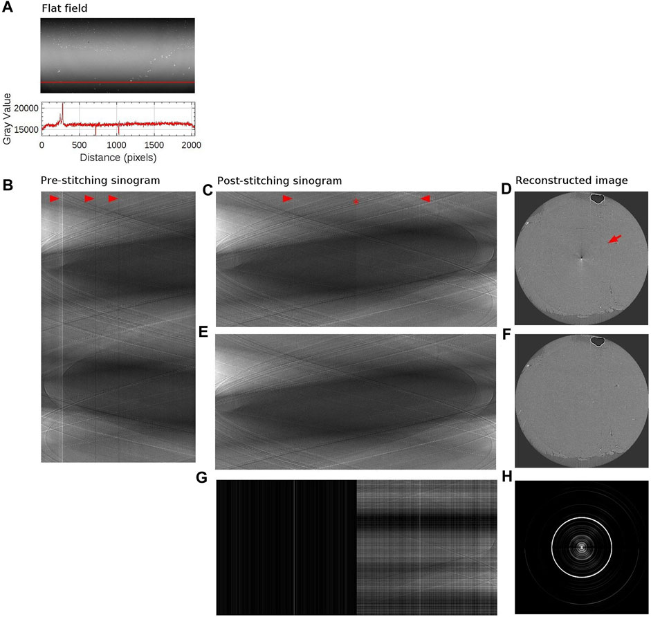
FIGURE 5. Sinogram stitching and ringing artifact removal. (A) The above image is a flat field image (matrix size: 1,000 × 2048). The detector matrix size is 2048 × 2048, but the edge rows are excluded in order to use beam within its full-width-at-half-maximum only. The bottom plot shows the intensity profile along the red vertical line. (B) Sinogram with a sample in place, at the level of the red vertical line, measured with half-acquisition mode (3,600 × 2048). 3,600 projections were acquired over 360° with offset center-of-rotation. Red arrows point to stripe artifacts which coincides with the intensity variation in the flat field image (C) Stitched sinogram (1800 × 3,732). Projections obtained at rotation angles 1°–180° have been stitched together with angles 181°–360° at the point indicated by a red star to yield the equivalent 180° sinogram. Stripe artifacts, occurring in agreement with variation in the flat field image, have been indicated by red arrows. (D) Reconstructed image from the sinogram shown in panel (C). Ringing artifact is indicated with a red arrow. Artifacts at the center of the image is due to half-acquisition mode. (E) Stitched sinogram (1800 × 3,732) obtained with ring removal filter and line-by-line normalization. (F) Reconstructed image from the sinogram shown in panel (E). (G) Intensity difference between panel (C,E). (H) Intensity difference between panel (D,F). The brightness and contrast were adjusted to better visualize the difference in panel (G,H).
A standardized reconstruction pipeline for propagation-based phase-contrast CT includes a pre-processing step for image normalization also known as flat-field correction, phase retrieval, potential filtering for ring removal and a reconstruction algorithm such as filtered back projection. In this section, we demonstrate how each process of the reconstruction steps can influence the final result.
The 3D reconstruction procedure (Step 3a–Step 3c) was done with SYRMEP Tomo Project (STP) software suite [46,47], which is developed based on the Astra toolbox [48]. At our home institution, we used a workstation with 64 GB memory, 12 GB of graphic memory, and 12 physical CPU cores. A raw projections datasets of size around 10 GB required 1 h from preprocessing to reconstruction with STP software. The reconstruction process from flat-fielding correction to image reconstruction can be automatized once the parameters for each step are defined. However, the computation time depends on the hardware resources (CPU and GPU).
Raw data from each acquisition can consist of tenths of GB. They are archived at Elettra server for several years and can be retrieved if requested. The output of the STP software is a stack of reconstructed slices in 32-bit TIFF file format. 1 μm isotropic voxel images scanned with half acquisition mode can amount to over 100 GB after reconstruction. Typically, in 3–5 days long beamtime, several TB of data can be produced.
For post-processing steps (Step 3d - Step 3f), we used a widely used software in the biology community, called ImageJ [49,50].
If the half acquisition method was used, the overlap should be estimated to perform sinogram stitching. The overlap can be estimated either using a Fourier-based algorithm [51] or by visual assessment. Typically, we first performed stitching using the algorithm and visually inspected the resulting sinogram. If the stitching result needed additional adjustment, we changed the parameter in small steps until the result improved. Usually, the overlap needed small correction for each vertical steps of the same lateral FOV.
Imperfect scintillators or defective pixels can be the source of ring artifacts in the reconstructed images. There are several ring artifact removal filters that can be tuned and tested. The strength of the ring removal filter can significantly reduce the artifacts, but can introduce blurring in the image. An alternative approach is to acquire images by introducing random shifts of a few pixels of either the detector or the sample during acquisitions, transforming ring artifact into dispersed noise [52]. This approach requires projections in the step-and-shoot mode, thus increasing the acquisition time.
When the FOV is significantly smaller than the entire sample, it is recommended to use padding on the sinogram in order to reduce the local tomography artefact [53].
To compensate for imperfect flat-fielding due to factors such as beam instabilities, or time varying detector properties, users may consider using dynamic flat-field correction [54].
In propagation based SR PhC-µCT, the phase signal is retrieved from the acquired projections prior to the 3D reconstruction. A widely used phase retrieval algorithm is the one developed by Paganin and colleagues (2002). The algorithm assumes that the sample under investigation is homogeneous and that the data is acquired with monochromatic radiation. It uses the ratio between the real (δ) and the imaginary part (β) of the refractive index as a parameter. Even when these conditions are not met, for non-homogeneous objects and polychromatic radiation, a common experimental practice is to use the algorithm parameters δ/β as a tuning parameter to regulate the strength of the filter and thus the blurring introduced in the image [38]. In practice, the algorithm acts like a low pass filter in the spatial frequency space. For FFPE brain samples, we used the δ/β in the range between 20 and 50 and obtained reproducible results across our unstained human tissue samples.
In this step, the matrix of the projections is used to calculate tomographic images. The STP software suite provides several reconstruction filters. This choice depends on the specific imaging application, as well as the desired trade-off between image sharpness and noise reduction. For this application, filtered back projection algorithm was applied using Shepp-Logan filter [47]. This algorithm is known to be fast and efficient when applied to datasets with good signal-to-noise ratio and a large number of projections. A circularly shaped reconstruction window can be applied to limit the result within the FOV (as shown in Figure 3C).
Due to the so called ‘beam hardening’ effect, images can exhibit a cupping artifact, which yields brighter intensity in the periphery than the inner region. The half-acquisition mode can also lead to cupping artifacts. There are several techniques to remove such artifacts. For example, we implemented slice-by-slice second degree polynomial fitting with the Xlib plugin [55] (Figure 6).
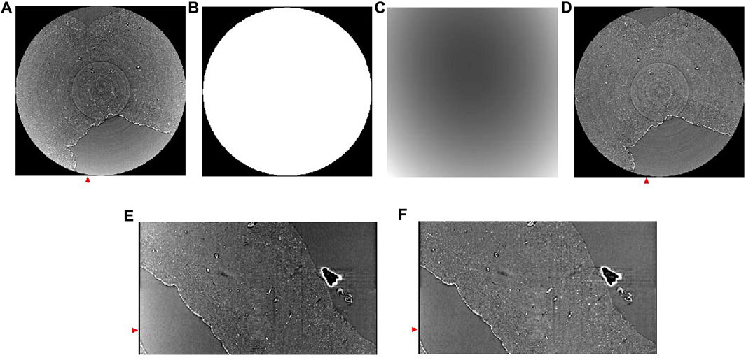
FIGURE 6. Background removal using polynomial fitting. (A) Reconstructed horizontal image showing cupping artifact. (B) Mask for background removal. (C) Background estimated using second degree polynomial fitting. (D) Corresponding slide shown in panel A after background removal. (E) A vertical slice of the image without background removal, taken from the region annotated with a red arrow in panel (A) (F) A vertical slice of the image after background removal, taken from the region annotated with a red arrow in panel (F). Red arrows in (E,F) match the position of the slides shown in panel (A,D).
This is an optional step for users who want to combine neighboring volumes into a single volume. The pairwise stitching function [56] is a useful tool for merging 3D images. This function uses the Fourier transform to calculate the translation matrix from the frequency domain. For the function to perform well, there should be enough overlap between two images that need to be stitched together.
This algorithm can also be used for registering the high resolution image to the low resolution image. For example, we used this function to register the 1 µm isotropic voxel size images to the 5 µm isotropic voxel size image. The higher resolution images should first be downscaled to match the voxel size of the lower resolution image.
In order to investigate the biological structures systematically and perform any volumetric quantitative measure, it is desirable to segment them. Manual segmentation requires a trained eye and a lot of time [39]. We suggest two segmentation approaches to automatically identify biological structures in SR PhC-µCT images: an intensity-based approach and an edge-based approach. These pipelines can be implemented with ImageJ plugins specialized for 3D image processing such as 3D ImageJ Suite [57] and MorphlibJ [58]. An example of a segmentation result using these methods are presented in Figure 7. These methods do not require training data or as much computational power as machine learning based approaches (mentioned in discussions).
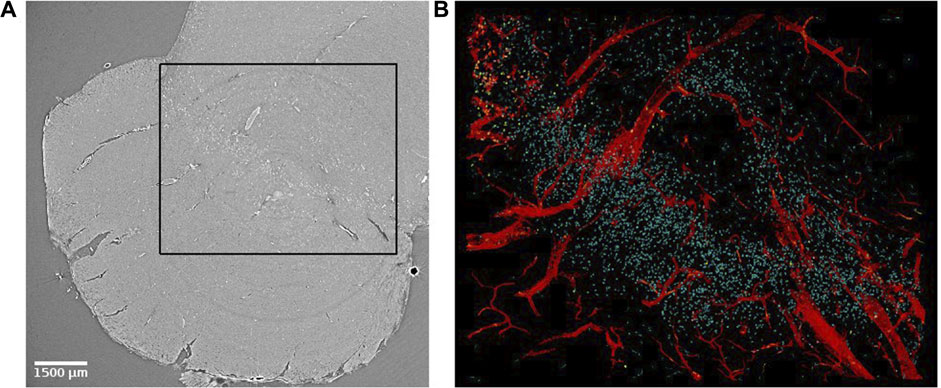
FIGURE 7. Virtual histology of the substantia nigra of the human brain stem. (A) Synchrotron radiation phase-contrast microtomography obtained with 4.74 µm isotropic voxel size. (B) Segmented results from the region indicated with a black rectangle in panel (A). Blood vessels (in red) were segmented using an edge-based approach [27]. Corpora amylacea (yellow) were segmented using an intensity-based approach [59] and a similar approach was used to identify neuromelanin (cyan). Corpora amylacea are clustered in the top left corner.
The intensity-based approach relies on the attenuation of X-ray dependent on the density and composition of the materials. Therefore, it is useful for identifying structures containing elements with high atomic weight (e.g., neuromelanin with iron) or dense structures (e.g., corpora amylacea). After applying a threshold to the image, the resulting image will be a binary image with many connected components. Morphological features of the connected components such as size and sphericity can be used to increase the accuracy of the segmentation [59].
The edge-based approach is suitable for detection of large connected structures such as blood vessels. Typically, a denoising process such as median filter precedes the edge detection algorithm. A median filter can remove salt-and-pepper noise while preserving edge structures. Deriche-Canny edge detection followed by a flood-filling process was proposed in our previous work [27].
With high resolution images amounting to large data sizes, users should consider working with down-sampled images. If the structure of interest is large enough, down-sampling can be used to reduce the computation time.
Histology is essential for validating the observed structure in SR PhC-µCT as known biological entities. The advantage is that histology can be performed on the same FFPE samples as those used for SR PhC-µCT. Using a rotational microtome (Leica, Wetzlar, Germany), we cut the paraffin block into ∼10 µm thick sections. These sections can be stained for investigating specific research topics.
It has been shown that X-ray exposure during SR PhC-µCT does not hinder subsequent histological analysis [21]. We have tested four types of classical staining methods that reliably work, including hematoxylin eosin stain and luxol fast blue stain. Table 2 summarizes how color appearance can be interpreted. In our experiments, immunohistochemical staining was not reliable, presumably due to prolonged formalin fixation. Among the antibodies that we have tested, anti-CD34 (a marker for endothelial cells) and anti-Aquaporin 4 antibodies were successful but ERG (ETS-Related Gene) antibodies were not. In typical research settings, small pieces of tissue is fixed in formalin for about 24 h. Since the samples we used were of ∼2 cm3 volume, longer storage in fixative solution was necessary. Commercial antibodies are likely not optimized for tissues stored in fixative solution for longer times. Furthermore, the differences in perfusion versus immersion fixation is known to influence antibody binding [60].
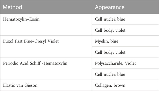
TABLE 2. List of histology methods. These techniques successfully worked for brain tissue that were scanned with synchrotron radiation imaging. The right column describes how the biological structures appear with the corresponding staining.
3D reconstruction of histological slides by serial alignment is very challenging due to non-linear deformation. Several methods have been proposed [61–63]. Besides, the registration of microscopy images to µCT images is also not trivial, since microscopy images are not isotropic as in microtomography [64]. We recommend using histology for characterizing biological components. How to do so is explained below.
In this section, we present biological features that can be extracted from SR PhC-µCT acquired from unstained human brain samples. Figure 7 demonstrates how multiple features can be extracted from a single PhC-µCT image. An automated segmentation pipeline was used to extract blood vessels, neuromelanin and corpora amylacea as explained in ‘Step 3f’. Each feature will be further discussed in the following paragraphs.
We mainly present our own measurements from FFPE samples acquired at SYRMEP beamline. For comparison, images from other open source data acquired at different synchrotron facilities are shown when applicable ([25,65]: PNAS). Note that variations in tissue preparation such as hydrated/dehydrated, embedding material, frozen, can change the contrast [24,65,66].
As we are not introducing an external contrast agent, the SR PhC-µCT signal relies on the intrinsic density and tissue composition [67]. Biological structures that are dense or contain materials with high electron density will lead to increased attenuation. Increased attenuation in a region implies that the structure is 1) composed of elements with high atomic weight (e.g., iron, zinc) and/or 2) are very densely packed.
It is challenging to investigate the blood vessel structure using traditional 2D histology, where the tissues are cut into thin slices before imaging. SR PhC-µCT can provide 3D isotropic images that preserve the continuity of the blood vessel. When exploring SR PhC-µCT data by simple visual inspection, the trajectories of large blood vessels are prevalent features one can easily notice (see Video 1).
Figure 8 shows examples of different brain regions measured with SR PhC-µCT, paired with segmented blood vessel structures. The brain stem acquired with 5 µm isotropic voxels (Figure 8A) was processed using the edge-based vessel segmentation method detailed in Lee et al. [27]. The resulting vessel map (Figure 8B) matches the known anatomy of the blood vessel in the region as previously reported [68]. For whole brain data, it is possible to follow the trajectory of the oxygenated blood from the heart by leveraging on the known blood source to the brain, called circle of Willis (Figure 8C). We used a semi-automated seed-based segmentation method with the ITK-SNAP software [69] to trace the arteries of a hemisphere by following arteries branching off from the circle of Willis (Figure 8D). Lastly, SR PhC-µCT of the occipital cortex (Figure 8E) was processed with an edge-based segmentation method to reveal the penetrating vessels running orthogonally to the surface of the cortex (Figure 8F).
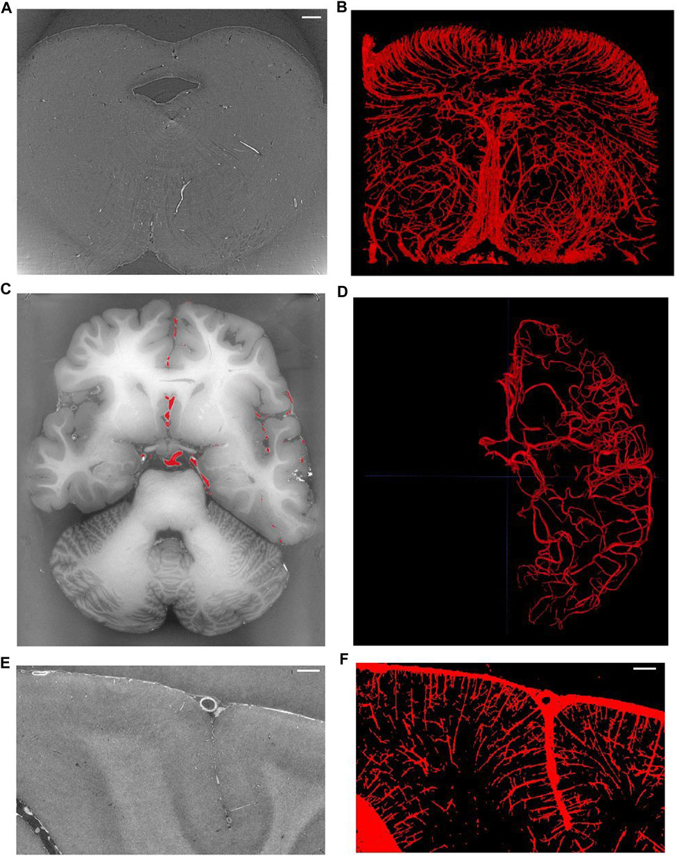
FIGURE 8. Vessel extraction from synchrotron radiation phase-contrast microtomography. (A). Axial view of the human brainstem. (B). Vessel segmentation using edge-based automated segmentation from the region shown in A (C). Axial view of the whole brain. (D) Result of artery tracing of one hemisphere using seed based semi-automated segmentation with ITK-SNAP. (E) Coronal view of the occipital lobe. (F) Vessel segmentation result using edge-based segmentation from the region shown in panel (E). Scale bars in A, E, F are 1 mm in length. (C–F) are based on open source human organ atlas data [25]. Panels B and D are 3D rendered views of a 1.5 mm thick slab and a hemisphere, respectively. Panel F is a maximum intensity projection across 1 mm depth. DOI identifier for (C) is 10.15151/ESRF-DC-572252655 and (E) is 10.15151/ESRF-DC-572253460.
Note that the appearance of blood vessels may be different in hydrated tissues ([37,65]: Biomed.Optics).
Some large neurons could be visualized with SR PhC-µCT. Figure 9 shows the large neurons of the mesenphalic trigeminal nucleus acquired with 5 μm and 1 µm isotropic voxels. Individual cells are sharply delineated only in the 1 µm isotropic voxel image. Figure 10 shows examples of smaller neurons observed with 1 µm isotropic voxel size. Histology of the matching region was used to validate these structures as neurons (Figures 10A–D). About the center of the cell body, the nucleolus appears as a hyperintense dot in all three examples, in agreement with prior studies ([37,70]: PNAS). However, the cytoplasm of the neurons showed different contrast with respect to the surrounding tissue. The signal in the cytoplasm was either isointense (Figures 10A, C), hyperintense (Figure 10E) or hypointense (Figure 10F) in comparison with the surrounding tissue. In one case, the edge of the neuron appeared darker than the surrounding and than the cytoplasm, possible due to local shrinkage, similar to what can be observed in blood vessels (Figure 10A). Further investigations are required to identify which intracellular components give rise to such contrast differences (e.g., organelles or cytoplasm). Nonetheless, this comparison of a few neurons already points towards the rich variety of features that can be observed in SR PhC-µCT images at the cellular level.
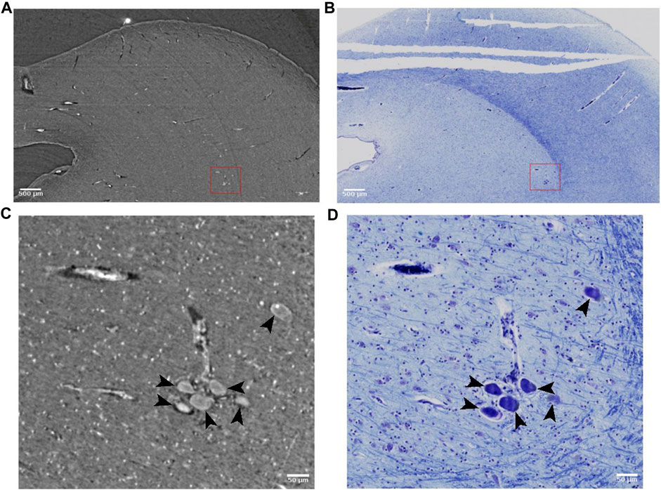
FIGURE 9. Large neurons detected with synchrotron radiation phase-contrast microtomography (SR PhC-µCT) and histology. (A) SR PhC-µCT acquired with 4.94 µm isotropic voxel size. (B) Histology of a field-of-view (FOV) matching panel (A). (C) SR PhC-µCT with 0.94 µm voxel size of the red rectangle region in panel (A). Black arrows point to large neurons. (D) Histology of the FOV matching panel (C). Scale bars (A,B) 500 μm (C,D) 50 µm.
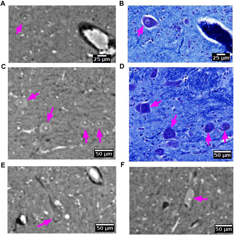
FIGURE 10. Neurons detected with synchrotron radiation phase-contrast microtomography (SR PhC-µCT). (A–D) Some neurons are found in both SR PhC-µCT and histology. The neuron in panel A shows the same intensity within the cytoplasm as in the surrounding tissue, whereas neurons in panel C show higher intensity in the cytoplasm. (E,F) Examples of neurons with different intensity within the cytoplasm, with lower intensity of cytoplasm shown in panel E and higher intensity observed in the cytoplasm in panel F. Histology of the matching regions were not available. The magenta arrows point to neurons in each panel. SR PhC-µCT are acquired with 0.94 µm isotropic voxel size.
Neuromelanin is a dark pigment that progressively accumulate in catecholaminergic neurons, such as dopaminergic neurons in the substantia nigra. In histological slides, neuromelanin appears naturally brown without any staining. It contains several elements with large atomic weight such as iron, zinc and selenium [71]. Hence, it is likely that neuromelanin gives rise to higher X-ray attenuation than that typically observed in the cytoplasm of neurons (Figure 11). Indeed, in the substantia nigra we observed very bright spots with shapes that were similar to histology sections of a matching part in substantia nigra. From the single specimen analyzed so far, it appears that the neuromelanin-containing part of the cytoplasm yields the strongest contrast.
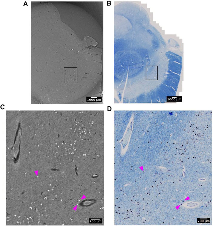
FIGURE 11. Neuromelanin in the dopaminergic neurons of the substantia nigra detected with synchrotron radiation phase-contrast microtomography (SR PhC-µCT). (A) SR PhC-µCT of the substantia nigra region acquired with 4.74 µm voxel size. (B) The histology of the matching region of panel (A). (C) A zoomed inset of rectangle in (A). Neuromelanin, annotated with magenta arrows, have outstanding contrast to the surrounding tissue. (D) A zoomed inset of rectangle in B, with neuromelanin annotated with magenta arrows. Scale bars (A,B) 1 mm. (C,D) 200 µm.
Corpora amylacea are polyglucosan granules that are found in multiple organs, including the brain [72]. They are under active investigation for their relationship to aging, neurodegeneration, immune system and glymphatic transport mechanisms in the brain. The current understanding is that CA is mostly composed of carbohydrates [73]. In SR PhC-µCT, these granules can be identified as hyperintense structures with a spherical shape (Figure 12, Supplementary Figure S4) [28]. Recently, a 3D distribution of CA within the human brain stem was analysed from four subjects with mean age of 76 years old, reporting an increased density in the dorsomedial column of the periaqueductal gray [59]. At the time being, the specificity of our CA detection method must be further investigated, since we anticipate that other densely packed spherical granules encountered in the brain such as Lewy bodies [74] may look similar to CA in SR PhC-µCT measurements. In future studies, such uncertainties can be investigated.
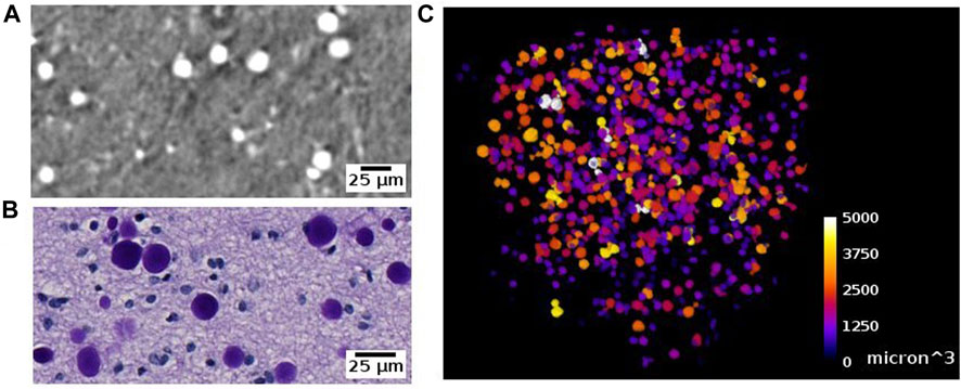
FIGURE 12. Corpora amylacea detected with synchrotron radiation phase-contrast microtomography (SR PhC-µCT) and histology. (A) Corpora amylace within the human brain tissue is visible in SR PhC-µCT (0.94 µm isotropic voxel). (B) The histology of an adjacent region of panel (A) (C) Segmentation result of corpora amylacea from SR PhC-µCT, color-coded by size of the granules.
We were able to observe some of fiber tracts. For example, the oculomotor nerve appeared as hyperintense against the surrounding tissue (Figure 13). FFPE samples may not be the best option for visualizing fiber structure. In a recent study using mouse brain samples showed that neuronal fibers have higher contrast after ethanol dehydration than after paraffin embedding ([75,76]: Journal of Neuroscience Methods). On the other hand, they also observed variations between different fibers. The attenuation coefficient of fibers in cerebellum was lower than fibers in the striatum. Since axonal density, diameter, and myelin thickness can vary considerably between brain regions, we cannot expect fiber tracts to show the same appearance across brain regions. A notable example are large white matter fiber tracts, where the myelin thickness increases linearly with increasing axonal diameter [77,78]. Using freeze drying, it has been shown that myelinated axonal tracts in the mouse striatum can be segmented from PhC-µCT images based on their specific attenuation coefficients in this tissue preparation [79].
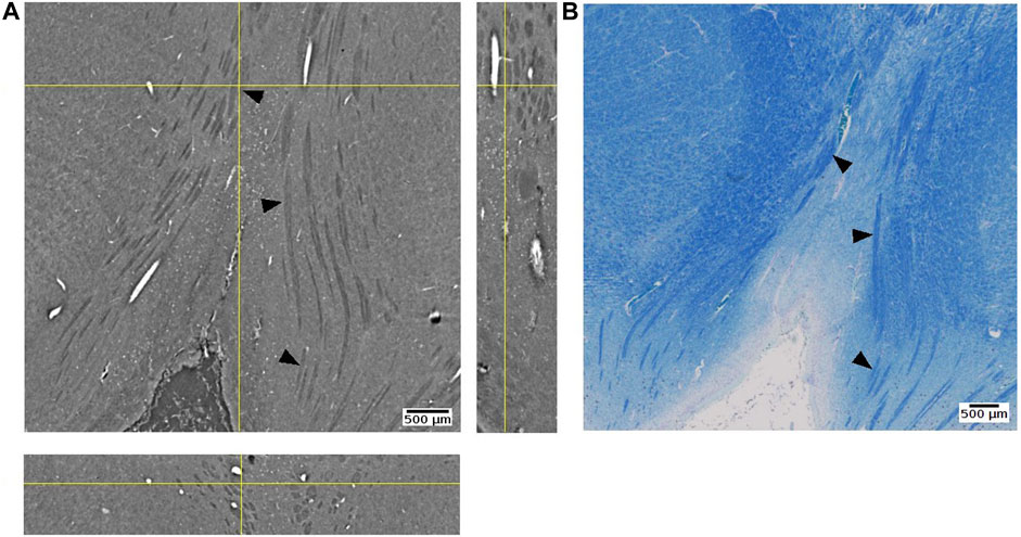
FIGURE 13. Oculomotor nerve detected with synchrotron radiation phase-contrast microtomography (SR PhC-µCT) and histology. (A) An orthogonal view of the posterior human midbrain acquired with SR PhC-µCT (4.74 µm isotropic voxel). The oculomotor nerve fibers appear as hypointense (B) Histology of the adjacent region stained with luxol fast blue-cresyl violet method. The fiber tracts appear in blue color, since myelin is stained with the luxol fast blue stain. Arrows point to examples of oculomotor nerve fibers in both imaging modalities.
This paper provides a step-by-step guideline for imaging unstained FFPE human brain tissue samples using SR PhC-µCT starting from tissue preparation and measurement to image processing. Although the protocol is written based on the SYRMEP beamline, it can also serve as a general guideline for potential users of other imaging beamlines. Reconstruction and post-processing workflow focus on graphic-user-interface based methods (e.g., STP, ImageJ, ITK-SNAP) to increase accessibility for a broad group of potential users. We also present an overview of biological features that can be identified from the unstained human brain ranging from blood vessel networks to intracellular components such as neuromelanin.
The protocol can be modified to enable particular research goals. Besides the propagation-based method, there are other phase contrast methods, such as grating interferometry or edge illumination techniques, that might be applied for human brain imaging. The grating interferometry provides more reliable estimates of phase shifts but requires longer measurement times and a more complex reconstruction process [30,80]. Edge illumination has potential for soft tissue imaging even in a laboratory setup but also requires longer measurement time [81]. These options may be considered for obtaining phase-contrast imaging of soft tissue using conventional X-ray systems. For the segmentation approach, we point towards the use of intensity threshold and morphometry based methods. On the other hand, machine learning segmentation methods such as U-Net [82] or the random tree algorithm [83] may be useful, if enough training data are available.
With the wide range of new brain imaging methods under development, there is a need for a gold standard method. Researchers within the neuroscience community are beginning to endorse phase contrast X-ray microtomography as a putative novel gold standard for structural imaging [84,85], along with cryo-electron microscopy. For example, microtomography has been used to validate angiography acquired from ultrasound localization microscopy [86]. Furthermore, SR PhC-µCT can show sub-cellular morphologies of neurons with no labeling [70].
Synchrotron radiation X-ray is unique for its light with high flux and spatial coherence, enabling the application of phase contrast techniques with fast acquisition times. However, it is limited by the scarce availability of sources, which leads to restricted access. In order for synchrotron radiation light sources to best serve science, users should be encouraged to make data available as open source [87]. It will reduce possible redundancy and allow acquisition of more samples by sharing of the workload between research groups. Some facilities such as the European Synchrotron Radiation Facility already provide user friendly portal services for accessing open data.
Developments in laboratory based PhC-µCT are projecting new possibilities as well. Microfocus X-ray sources from liquid-metal jet sources provide partially coherent light that enables phase contrast imaging. The feasibility for imaging down to the cellular level has already been demonstrated ([88]: PNAS). If the time required for measurement and reconstruction is reduced to below 1 hour, the technique may even enable intra-operative imaging [89]. Success of surgical removal of tumor cells may be assessed during surgery by imaging of the resection margins [90].
The future of SR PhC-µCT for imaging unstained human brain samples has great potential [86]. To the best of our knowledge, there is only one dataset of a whole human brain available at the moment, which has been acquired with 25 µm isotropic voxel size [25]. This voxel size allows for identifying large blood vessels and delineating the boundary between grey and white matter. However, it is too large for investigating the brain at a cellular level. Ideally, whole human brain samples should be scanned at high resolution as done recently with the mouse brain [75]: SPIE). Higher resolution images combined with automatic cell classification is likely to become a great resource for understanding the human brain at an advanced level of detail ([65]: PNAS). With further improvements, SR PhC-µCT has the potential to provide unprecedented insights into human brain anatomy and neurological diseases.
The original contributions presented in the study are included in the article/Supplementary Material, further inquiries can be directed to the corresponding author.
The studies involving humans were approved by the Medical Department of the University of Tübingen. The studies were conducted in accordance with the local legislation and institutional requirements. The participants provided their written informed consent to participate in this study.
JL: Conceptualization, Data curation, Investigation, Methodology, Project administration, Writing–original draft, Writing–review and editing. SD: Conceptualization, Investigation, Methodology, Software, Writing–original draft, Writing–review and editing. AM: Resources, Writing–review and editing. UM: Resources, Validation, Writing–review and editing. GT: Data curation, Investigation, Resources, Writing–review and editing. EL: Data curation, Investigation, Resources, Writing–review and editing. LD’A: Writing–review and editing. SM: Investigation, Writing–review and editing. TS: Resources, Writing–review and editing. JB: Funding acquisition, Writing–review and editing. KS: Funding acquisition, Writing–review and editing. RL: Conceptualization, Investigation, Methodology, Writing–original draft, Writing–review and editing. GH: Conceptualization, Data curation, Funding acquisition, Investigation, Methodology, Project administration, Supervision, Writing–original draft, Writing–review and editing.
The author(s) declare financial support was received for the research, authorship, and/or publication of this article. Open Access funding was enabled and organized by Projekt DEAL. We acknowledge Elettra Sincrotrone Trieste, Max Planck Society and the Federal Ministry of Education and Research (BMBF Grant 01GQ2101) for financial support. SD has been supported by the “AIM: Attraction and International Mobility”—PON R&I 2014–2020 Calabria and “Progetto STAR 2”—PIR01_00008)—Italian Ministry of University and Research.
We acknowledge Elettra Sincrotrone Trieste for providing access to its synchrotron radiation facilities and we thank Diego Dreossi for the cone beam imaging of our samples. We thank Johannes Steiner and Tatjana Steiner from the body donor program, Jürgen Papp, Andreas Wagner, and Peter Neckel for organ handling and Henry Evrard, Alina Novitska, Mark Bailey and Lucas Gehlhaar for support with the Zeiss Axioscan Microscope. Finally, we would like to express our gratitude to the body donors.
The authors declare that the research was conducted in the absence of any commercial or financial relationships that could be construed as a potential conflict of interest.
All claims expressed in this article are solely those of the authors and do not necessarily represent those of their affiliated organizations, or those of the publisher, the editors and the reviewers. Any product that may be evaluated in this article, or claim that may be made by its manufacturer, is not guaranteed or endorsed by the publisher.
The Supplementary Material for this article can be found online at: https://www.frontiersin.org/articles/10.3389/fphy.2023.1335285/full#supplementary-material
1. Adler DH, Pluta J, Kadivar S, Craige C, Gee JC, Avants BB, et al. Histology-derived volumetric annotation of the human hippocampal subfields in postmortem MRI. Neuroimage (2014) 84:505–23. doi:10.1016/j.neuroimage.2013.08.067
2. Amunts K, Mohlberg H, Bludau S, Zilles K. Julich-Brain: a 3D probabilistic atlas of the human brain’s cytoarchitecture. Science (2020) 369(988):988–92. doi:10.1126/science.abb4588
3. Tendler BC, Hanayik T, Ansorge O, Bangerter-Christensen S, Berns GS, Bertelsen MF, et al. The Digital Brain Bank, an open access platform for post-mortem imaging datasets. Elife (2022) 11(2022):e73153. doi:10.7554/elife.73153
4. Mai H, Luo J, Hoeher L, Al-Maskari R, Horvath I, Chen Y, et al. Whole-body cellular mapping in mouse using standard IgG antibodies. Nat Biotechnol (2023) 1–11. doi:10.1038/s41587-023-01846-0
5. Park J, Wang J, Guna W. Integrated platform for multi-scale molecular imaging and phenotyping of the human brain. bioRxiv (2022) 2022–03. doi:10.1101/2022.03.13.484171
6. Edlow BL, Mareyam A, Horn A, Polimeni JR, Witzel T, Tisdall MD, et al. 7 Tesla MRI of the ex vivo human brain at 100 micron resolution. Scientific data (2019) 6(1):244. doi:10.1038/s41597-019-0254-8
7. Shepherd TM, Hoch MJ, Bruno M, Faustin A, Papaioannou A, Jones SE, et al. Inner SPACE: 400-micron isotropic resolution MRI of the human brain. Front Neuroanat (2020) 14:9. doi:10.3389/fnana.2020.00009
8. Tuzzi E, Balla DZ, Loureiro JR, Neumann M, Laske C, Pohmann R, et al. Ultra-high field MRI in Alzheimer’s disease: effective transverse relaxation rate and quantitative susceptibility mapping of human brain in vivo and ex vivo compared to histology. J Alzheimer's Dis (2020) 73(4):1481–99. doi:10.3233/jad-190424
9. Flint JJ, Menon K, Hansen B, Forder J, Blackband SJ. Visualization of live, mammalian neurons during Kainate-infusion using magnetic resonance microscopy. Neuroimage (2020) 219:116997. doi:10.1016/j.neuroimage.2020.116997
10. Handwerker J, Pérez-Rodas M, Beyerlein M, Vincent F, Beck A, Freytag N, et al. A CMOS NMR needle for probing brain physiology with high spatial and temporal resolution. Nat Methods (2020) 17(1):64–7. doi:10.1038/s41592-019-0640-3
11. Birkl C, Langkammer C, Golob-Schwarzl N, Leoni M, Haybaeck J, Goessler W, et al. Effects of formalin fixation and temperature on MR relaxation times in the human brain. NMR Biomed (2016) 29(4):458–65. doi:10.1002/nbm.3477
12. Dusek P, Madai VI, Huelnhagen T, Bahn E, Matej R, Sobesky J, et al. The choice of embedding media affects image quality, tissue R2*, and susceptibility behaviors in post-mortem brain MR microscopy at 7.0 T. Magn Reson Med (2019) 81(4):2688–701. doi:10.1002/mrm.27595
13. Nazemorroaya A, Aghaeifar A, Shiozawa T, Hirt B, Schulz H, Scheffler K, et al. Developing formalin-based fixative agents for post mortem brain MRI at 9.4 T. Magn Reson Med (2022) 87(5):2481–94. doi:10.1002/mrm.29122
14. Xue S, Gong H, Jiang T, Luo W, Meng Y, Liu Q, et al. Indian-ink perfusion based method for reconstructing continuous vascular networks in whole mouse brain. PloS one (2014) 9(1):e88067. doi:10.1371/journal.pone.0088067
15. Wälchli T, Bisschop J, Miettinen A, Ulmann-Schuler A, Hintermüller C, Meyer EP, et al. Hierarchical imaging and computational analysis of three-dimensional vascular network architecture in the entire postnatal and adult mouse brain. Nat Protoc (2021) 16(10):4564–610. doi:10.1038/s41596-021-00587-1
16. Wehrse E, Klein L, Rotkopf LT, Stiller W, Finke M, Echner GG, et al. Ultrahigh resolution whole body photon counting computed tomography as a novel versatile tool for translational research from mouse to man. Z für Medizinische Physik (2023) 33 (2):155–67. doi:10.1016/j.zemedi.2022.06.002
18. Peterzol A, Olivo A, Rigon L, Pani S, Dreossi D. The effects of the imaging system on the validity limits of the ray-optical approach to phase contrast imaging. Med Phys (2005) 32(12):3617–27. doi:10.1118/1.2126207
19. Paganin D, Mayo SC, Gureyev TE, Miller PR, Wilkins SW. Simultaneous phase and amplitude extraction from a single defocused image of a homogeneous object. J Microsc (2002) 206(1):33–40. doi:10.1046/j.1365-2818.2002.01010.x
20. Brombal L. Effectiveness of X-ray phase-contrast tomography: effects of pixel size and magnification on image noise. J Instrum (2020) 15(01):C01005. doi:10.1088/1748-0221/15/01/C01005
21. Saccomano M, Albers J, Tromba G, Dobrivojević Radmilović M, Gajović S, Alves F, et al. Synchrotron inline phase contrast µCT enables detailed virtual histology of embedded soft-tissue samples with and without staining. J synchrotron Radiat (2018) 25(4):1153–61. doi:10.1107/S1600577518005489
22. Müller B, Khimchenko A, Rodgers G, Osterwalder M, Tanner C, Schulz G. X-ray imaging of human brain tissue down to the molecule level. In: International Conference on X-Ray Lasers 2020, 11886:298–307. SPIE (2021).
23. Peña LA, Donato S, Bonazza D. Multiscale X-ray phase-contrast tomography: from breast CT to micro-CT for virtual histology. Physica Med (2023) 112:102640. doi:10.1016/j.ejmp.2023.102640
24. Rodgers G, Kuo W, Schulz G, Scheel M, Migga A, Bikis C, et al. Virtual histology of an entire mouse brain from formalin fixation to paraffin embedding. Part 1: data acquisition, anatomical feature segmentation, tracking global volume and density changes. J Neurosci Methods (2021) 364(2021):109354. doi:10.1016/j.jneumeth.2021.109354
25. Walsh CL, Tafforeau P, Wagner WL, Jafree DJ, Bellier A, Werlein C, et al. Imaging intact human organs with local resolution of cellular structures using hierarchical phase-contrast tomography. Nat Methods (2021) 18:1532–1541. doi:10.1038/s41592-021-01317-x
26. Einarsson E, Pierantoni M, Novak V, Svensson J, Isaksson H, Englund M. Phase-contrast enhanced synchrotron micro-tomography of human meniscus tissue. Osteoarthritis and Cartilage (2022) 30(9):1222–33. doi:10.1016/j.joca.2022.06.003
27. Lee JY, Mack AF, Shiozawa T, Longo R, Tromba G, Scheffler K, et al. Microvascular imaging of the unstained human superior colliculus using synchrotron-radiation phase-contrast microtomography. Scientific Rep (2022) 12(1):9238. doi:10.1038/s41598-022-13282-2
28. Hieber SE, Bikis C, Khimchenko A, Schweighauser G, Hench J, Chicherova N, et al. Tomographic brain imaging with nucleolar detail and automatic cell counting. Scientific Rep (2016) 6(1):32156. doi:10.1038/srep32156
29. Frost J, Schmitzer B, Töpperwien M, Eckermann M, Franz J, Stadelmann C, et al. 3d virtual histology reveals pathological alterations of cerebellar granule cells in multiple sclerosis. Neuroscience (2023) 520:18–38. doi:10.1016/j.neuroscience.2023.04.002
30. Astolfo A, Lathuilière A, Laversenne V, Schneider B, Stampanoni M. Amyloid-β plaque deposition measured using propagation-based X-ray phase contrast CT imaging. J synchrotron Radiat (2016) 23(3):813–9. doi:10.1107/s1600577516004045
31. Töpperwien M, van der Meer F, Stadelmann C, Salditt T. Correlative x-ray phase-contrast tomography and histology of human brain tissue affected by Alzheimer’s disease. Neuroimage (2020) 210:116523. doi:10.1016/j.neuroimage.2020.116523
32. Bukreeva I, Junemann O, Cedola A, Brun F, Longo E, Tromba G, et al. Micro-morphology of pineal gland calcification in age-related neurodegenerative diseases. Med Phys (2022) 50(3):1601–13. doi:10.1002/mp.16080
33. Junemann O, Ivanova AG, Bukreeva I, Zolotov DA, Fratini M, Cedola A, et al. Comparative study of calcification in human choroid plexus, pineal gland, and habenula. Cel Tissue Res (2023) 393:537–45. doi:10.1007/s00441-023-03800-7
34. Orhan K, Karla de FV, Gaêta-Araujo H. Artifacts in micro-CT. In: Micro-computed tomography (micro-CT) in medicine and engineering. Switzerland: Springer Nature (2020). p. 35–48.
35. Wehrl HF, Bezrukov I, Wiehr S, Lehnhoff M, Fuchs K, Mannheim JG, et al. Assessment of murine brain tissue shrinkage caused by different histological fixatives using magnetic resonance and computed tomography imaging. Histology and Histopathology (2015) 30(5):601–13. doi:10.14670/HH-30.601
36. De Guzman , Elizabeth A, Gleave JA, Nieman BJ. Variations in post-perfusion immersion fixation and storage alter MRI measurements of mouse brain morphometry. Neuroimage (2016) 142:687–95. doi:10.1016/j.neuroimage.2016.06.028
37. Eckermann M, Van der Meer F, Cloetens P, Ruhwedel T, Möbius W, Stadelmann C, et al. Three-dimensional virtual histology of the cerebral cortex based on phase-contrast X-ray tomography. Biomed Opt express (2021) 12(12):7582–98. doi:10.1364/boe.434885
38. Strotton MC, Bodey AJ, Wanelik K, Darrow MC, Medina E, Hobbs C, et al. Optimising complementary soft tissue synchrotron X-ray microtomography for reversibly-stained central nervous system samples. Scientific Rep (2018) 8(1):12017. doi:10.1038/s41598-018-30520-8
39. Saiga R, Uesugi M, Takeuchi A, Uesugi K, Suzuki Y, Takekoshi S, et al. Brain capillary structures of schizophrenia cases and controls show a correlation with their neuron structures. Scientific Rep (2021) 11(1):11768. doi:10.1038/s41598-021-91233-z
40. Zhanmu O, Yang X, Gong H, Li X. Paraffin-embedding for large volume bio-tissue. Scientific Rep (2020) 10(1):12639. doi:10.1038/s41598-020-68876-5
41. Brunet J, Walsh CL, Wagner WL, Bellier A, Werlein C, Marussi S, et al. Preparation of large biological samples for high-resolution, hierarchical, synchrotron phase-contrast tomography with multimodal imaging compatibility. Nat Protoc (2023) 18(5):1441–61. doi:10.1038/s41596-023-00804-z
42. Dullin C, di Lillo F, Svetlove A, Albers J, Wagner W, Markus A, et al. Multiscale biomedical imaging at the SYRMEP beamline of Elettra-Closing the gap between preclinical research and patient applications. Phys Open (2021) 6(2021):100050. doi:10.1016/j.physo.2020.100050
43. Donato S, Peña LA, Bonazza D, Formoso V, Longo R, Tromba G, et al. Optimization of pixel size and propagation distance in X-ray phase-contrast virtual histology. J Instrumentation (2022) 17(05):C05021. doi:10.1088/1748-0221/17/05/c05021
44. Lecoq P. Development of new scintillators for medical applications. Nucl Instr Methods Phys Res Section A: Acc Spectrometers, Detectors Associated Equipment (2016) 809:130–9. doi:10.1016/j.nima.2015.08.041
45. Wang G. X-ray micro-CT with a displaced detector array. Med Phys (2002) 29(7):1634–6. doi:10.1118/1.1489043
46. Brun F, Pacilè S, Accardo A, Kourousias G, Dreossi D, Mancini L, et al. Enhanced and flexible software tools for X-ray computed tomography at the Italian synchrotron radiation facility Elettra. Fundamenta Informaticae (2015) 141(2-3):233–43. doi:10.3233/fi-2015-1273
47. Brun F, Massimi L, Fratini M, Dreossi D, Billé F, Accardo A, et al. SYRMEP Tomo Project: a graphical user interface for customizing CT reconstruction workflows. Adv Struct Chem Imaging (2017) 3(1):4–9. doi:10.1186/s40679-016-0036-8
48. Van Aarle W, Palenstijn WJ, De Beenhouwer J, Altantzis T, Bals S, Batenburg KJ, et al. The ASTRA Toolbox: a platform for advanced algorithm development in electron tomography. Ultramicroscopy (2015) 157:35–47. doi:10.1016/j.ultramic.2015.05.002
49. Schneider CA, Rasband WS, Eliceiri KW. NIH Image to ImageJ: 25 years of image analysis. Nat Methods (2012) 9(7):671–5. doi:10.1038/nmeth.2089
50. Schindelin J, Arganda-Carreras I, Frise E, Kaynig V, Longair M, Pietzsch T, et al. Fiji: an open-source platform for biological-image analysis. Nat Methods (2012) 9(7):676–82. doi:10.1038/nmeth.2019
51. Vo NT, Drakopoulos M, Atwood RC, Reinhard C. Reliable method for calculating the center of rotation in parallel-beam tomography. Opt express (2014) 22(16):19078–86. doi:10.1364/oe.22.019078
52. Liu Y, Wei C, Xu Q. Detector shifting and deep learning based ring artifact correction method for low-dose CT. Med Phys (2023) 50:4308–24. doi:10.1002/mp.16225
53. Marone F, Münch B, Stampanoni M. Fast reconstruction algorithm dealing with tomography artifacts. Dev X-ray Tomography VII (2010) 7804. SPIE. doi:10.1117/12.859703
54. Van Nieuwenhove V, De Beenhouwer J, De Carlo F, Mancini L, Marone F, Sijbers J. Dynamic intensity normalization using eigen flat fields in X-ray imaging. Opt express (2015) 23(21):27975–89. doi:10.1364/oe.23.027975
55. Münch B, Trtik P, Marone F, Stampanoni M. Stripe and ring artifact removal with combined wavelet—Fourier filtering. Opt express (2009) 17(10):8567–91. doi:10.1364/oe.17.008567
56. Preibisch S, Saalfeld S, Tomancak P. Globally optimal stitching of tiled 3D microscopic image acquisitions. Bioinformatics (2009) 25(11):1463–5. doi:10.1093/bioinformatics/btp184
57. Ollion J, Cochennec J, Loll F, Escudé C, Boudier T. TANGO: a generic tool for high-throughput 3D image analysis for studying nuclear organization. Bioinformatics (2013) 29(14):1840–1. doi:10.1093/bioinformatics/btt276
58. Legland D, Arganda-Carreras I, Andrey P. MorphoLibJ: integrated library and plugins for mathematical morphology with ImageJ. Bioinformatics (2016) 32(22):3532–4. doi:10.1093/bioinformatics/btw413
59. Lee JY, Mack AF, Mattheus U, Donato S, Longo R, Tromba G, et al. Distribution of corpora amylacea in the human midbrain: using synchrotron radiation phase-contrast microtomography, high-field magnetic resonance imaging and histology. Front Neurosci (2023) 17:1236876. doi:10.3389/fnins.2023.1236876
60. Woelfle S, Deshpande D, Feldengut S, Braak H, Del Tredici K, Roselli F, et al. CLARITY increases sensitivity and specificity of fluorescence immunostaining in long-term archived human brain tissue. BMC Biol (2023) 21(1):113–28. doi:10.1186/s12915-023-01582-6
61. Amunts K, Lepage C, Borgeat L, Mohlberg H, Dickscheid T, Rousseau MÉ, et al. BigBrain: an ultrahigh-resolution 3D human brain model. science (2013) 340(6139):1472–5. doi:10.1126/science.1235381
62. Haddad TS, Friedl P, Farahani N, Treanor D, Zlobec I, Nagtegaal I. Tutorial: methods for three-dimensional visualization of archival tissue material. Nat Protoc (2021) 16(11):4945–62. doi:10.1038/s41596-021-00611-4
63. Howard AFD, Huszar IN, Smart A, Cottaar M, Daubney G, Hanayik T, et al. An open resource combining multi-contrast MRI and microscopy in the macaque brain. Nat Commun (2023) 14(1):4320. doi:10.1038/s41467-023-39916-1
64. Albers J, Svetlove A, Alves J, Kraupner A, di Lillo F, Markus MA, et al. Elastic transformation of histological slices allows precise co-registration with microCT data sets for a refined virtual histology approach. Scientific Rep (2021) 11(1):10846. doi:10.1038/s41598-021-89841-w
65. Eckermann M, Schmitzer B, van der Meer F, Franz J, Hansen O, Stadelmann C, et al. Three-dimensional virtual histology of the human hippocampus based on phase-contrast computed tomography. Proc Natl Acad Sci (2021) 118(48):e2113835118. doi:10.1073/pnas.2113835118
66. Töpperwien M, Markus A, Alves F, Salditt T. Contrast enhancement for visualizing neuronal cytoarchitecture by propagation-based x-ray phase-contrast tomography. NeuroImage (2019) 199:70–80. doi:10.1016/j.neuroimage.2019.05.043
67. Piai A, Contillo A, Arfelli F, Bonazza D, Brombal L, Assunta Cova M, et al. Quantitative characterization of breast tissues with dedicated CT imaging. Phys Med Biol (2019) 64(15):155011. doi:10.1088/1361-6560/ab2c29
68. Naidich TP, Duvernoy HM, Delman BN, Sorensen AG, Kollias SS, Haacke EM. Duvernoy’s atlas of the human brain stem and cerebellum. Springer Vienna (2009). doi:10.1007/978-3-211-73971-6
69. Yushkevich PA, Piven J, Hazlett HC, Smith RG, Ho S, Gee JC, et al. User-guided 3D active contour segmentation of anatomical structures: significantly improved efficiency and reliability. Neuroimage (2006) 31(3):1116–28. doi:10.1016/j.neuroimage.2006.01.015
70. Khimchenko A, Bikis C, Pacureanu A, Hieber SE, Thalmann P, Deyhle H, et al. Hard X-ray nanoholotomography: large-scale, label-free, 3D neuroimaging beyond optical limit. Adv Sci (2018) 5(6):1700694. doi:10.1002/advs.201700694
71. Bohic S, Murphy K, Paulus W, Cloetens P, Salomé M, Susini J, et al. Intracellular chemical imaging of the developmental phases of human neuromelanin using synchrotron X-ray microspectroscopy. Anal Chem (2008) 80(24):9557–66. doi:10.1021/ac801817k
72. Riba M, del Valle J, Augé E, Vilaplana J, Pelegrí C. From corpora amylacea to wasteosomes: history and perspectives. Ageing Res Rev (2021) 72:101484. doi:10.1016/j.arr.2021.101484
73. Sakai M, Austin J, Witmer F, Trueb L. Studies of corpora amylacea: I. Isolation and preliminary characterization by chemical and histochemical techniques. Arch Neurol (1969) 21(5):526–44. doi:10.1001/archneur.1969.00480170098011
74. Koh S-B, Suh S, Lee D, Kim A, Oh C, Yoon J, et al. Phase contrast radiography of Lewy bodies in Parkinson disease. Neuroimage (2006) 32(2):566–9. doi:10.1016/j.neuroimage.2006.04.217
75. Rodgers G, Tanner C, Schulz G. Mosaic microtomography of a full mouse brain with sub-µm pixel size. In: Proceeding of the Developments in X-Ray Tomography XIV, 12242 (2022).
76. Rodgers G, Tanner C, Schulz G, Migga A, Kuo W, Bikis C, et al. Virtual histology of an entire mouse brain from formalin fixation to paraffin embedding. Part 2: volumetric strain fields and local contrast changes. J Neurosci Methods (2022) 365(2022):109385. doi:10.1016/j.jneumeth.2021.109385
77. Liewald D, Miller R, Logothetis N, Wagner HJ, Schüz A. Distribution of axon diameters in cortical white matter: an electron-microscopic study on three human brains and a macaque. Biol Cybernetics (2014) 108:541–57. doi:10.1007/s00422-014-0626-2
78. Snaidero N, Schifferer M, Mezydlo A, Zalc B, Kerschensteiner M, Misgeld T. Myelin replacement triggered by single-cell demyelination in mouse cortex. Nat Commun (2020) 11(1):4901. doi:10.1038/s41467-020-18632-0
79. Mizutani R, Saiga R, Ohtsuka M, Miura H, Hoshino M, Takeuchi A, et al. Three-dimensional X-ray visualization of axonal tracts in mouse brain hemisphere. Scientific Rep (2016) 6(1):35061. doi:10.1038/srep35061
80. Lang S, Zanette I, Dominietto M, Langer M, Rack A, Schulz G, et al. Experimental comparison of grating-and propagation-based hard X-ray phase tomography of soft tissue. J Appl Phys (2014) 116:15. doi:10.1063/1.4897225
81. Olivo A. Edge-illumination x-ray phase-contrast imaging. J Phys Condensed Matter (2021) 33(36):363002. doi:10.1088/1361-648x/ac0e6e
82. Falk T, Mai D, Bensch R, Çiçek Ö, Abdulkadir A, Marrakchi Y, et al. U-Net: deep learning for cell counting, detection, and morphometry. Nat Methods (2019) 16(1):67–70. doi:10.1038/s41592-018-0261-2
83. Arganda-Carreras I, Kaynig V, Rueden C, Eliceiri KW, Schindelin J, Cardona A, et al. Trainable Weka Segmentation: a machine learning tool for microscopy pixel classification. Bioinformatics (2017) 33(15):2424–6. doi:10.1093/bioinformatics/btx180
84. Andersson M, Kjer HM, Rafael-Patino J, Pacureanu A, Pakkenberg B, Thiran JP, et al. Axon morphology is modulated by the local environment and impacts the noninvasive investigation of its structure–function relationship. Proc. Natl. Acad. Sci (2020) 117(52):33649–33659.
85. Kuan AT, Phelps JS, Thomas LA, Nguyen TM, Han J, Chen CL, et al. Dense neuronal reconstruction through X-ray holographic nano-tomography. Nat Neurosci (2020) 23(12):1637–1643. doi:10.1038/s41593-020-0704-9
86. Chavignon A, Heiles B, Hingot V, Orset C, Vivien D, Couture O, et al. 3D transcranial ultrasound localization microscopy in the rat brain with a multiplexed matrix probe. IEEE. Trans. Biomed. Eng. (2021) 69(7):2132–2142.
87. Bicarregui J, Matthews B, Frank S. PaNdata: open data infrastructure for photon and neutron sources. Synchrotron Radiat News (2015) 28(2):30–5. doi:10.1080/08940886.2015.1013418
88. Töpperwien M, van der Meer F, Stadelmann C, Salditt T. Three-dimensional virtual histology of human cerebellum by X-ray phase-contrast tomography. Proc Natl Acad Sci (2018) 115(27):6940–5. doi:10.1073/pnas.1801678115
89. Partridge T, Massimi L, Wolfson P, Jiang J, Astolfo A, Suaris T, et al. Intra-operative assessment of cancer with x-ray phase contrast computed tomography. In Developments in X-Ray Tomography XIV (2022) 12242: SPIE.
90. Twengström W, Moro CF, Romell J, Larsson JC, Sparrelid E, Björnstedt M, et al. Can laboratory x-ray virtual histology provide intraoperative 3D tumor resection margin assessment? J Med Imaging (2022) 9(3):031503. doi:10.1117/1.jmi.9.3.031503
Keywords: X-ray phase-contrast microtomography, virtual histology, synchrotron radiation X-ray, soft-tissue imaging, 3D imaging
Citation: Lee JY, Donato S, Mack AF, Mattheus U, Tromba G, Longo E, D’Amico L, Mueller S, Shiozawa T, Bause J, Scheffler K, Longo R and Hagberg GE (2024) Protocol for 3D virtual histology of unstained human brain tissue using synchrotron radiation phase-contrast microtomography. Front. Phys. 11:1335285. doi: 10.3389/fphy.2023.1335285
Received: 08 November 2023; Accepted: 18 December 2023;
Published: 08 January 2024.
Edited by:
Silvia Capuani, National Research Council (CNR), ItalyReviewed by:
Victor Asadchikov, Federal Scientific Research Centre Crystallography and Photonics (RAS), RussiaCopyright © 2024 Lee, Donato, Mack, Mattheus, Tromba, Longo, D’Amico, Mueller, Shiozawa, Bause, Scheffler, Longo and Hagberg. This is an open-access article distributed under the terms of the Creative Commons Attribution License (CC BY). The use, distribution or reproduction in other forums is permitted, provided the original author(s) and the copyright owner(s) are credited and that the original publication in this journal is cited, in accordance with accepted academic practice. No use, distribution or reproduction is permitted which does not comply with these terms.
*Correspondence: Ju Young Lee, anUueW91bmcubGVlQHR1ZWJpbmdlbi5tcGcuZGU=
†These authors share last authorship
Disclaimer: All claims expressed in this article are solely those of the authors and do not necessarily represent those of their affiliated organizations, or those of the publisher, the editors and the reviewers. Any product that may be evaluated in this article or claim that may be made by its manufacturer is not guaranteed or endorsed by the publisher.
Research integrity at Frontiers
Learn more about the work of our research integrity team to safeguard the quality of each article we publish.