Forecasting and dynamical modeling of reversible enzymatic reactions with a hybrid proportional fractional derivative

Chemical kinetics is a branch of chemistry that investigates the rates of chemical reactions and has applications in cosmology, geology, and physiology. In this study, we develop a mathematical model for chemical reactions based on enzyme dynamics and kinetics, which is a two-step substrate–enzyme reversible reaction, applying chemical kinetics-based modeling of enzyme functions. The non-linear differential equations are transformed into fractional-order systems utilizing the constant proportional Caputo–Fabrizio (CPCF) and constant proportional Atangana–Baleanu–Caputo (CPABC) operators. The system of fractional differential equations is simulated using the Laplace–Adomian decomposition method at different fractional orders through simulations and numerical results. Both qualitative and quantitative analyses such as boundedness, positivity, unique solution, and feasible concentration for the proposed model with different hybrid operators are provided. The stability analysis of the proposed scheme is also verified using Picard’s stable condition through the fixed point theorem.

1 Introduction

Catalysts are protein-based molecules that convert substrates into products. Specificity, catalytic activity, and control are all critical and result in a more efficient chemical reaction. Enzymes reduce the reaction-free energy of activation by converting substrates into products. They can strengthen chemical bonds between molecules by resolving forces. Enzymes are highly specialized, catalyzing only a small percentage of closely related substrate reactions, and they speed up chemical reactions by at least 10 million times. Enzyme kinetics is a study of the rates of enzyme-catalyzed chemical reactions [1]. Enzymes, like all efficient catalysts, significantly accelerate a specific reaction. The quantification, statistical formulation, and coefficients associated with this reaction rate are the primary subjects of enzyme kinetics [2]. Enzyme kinetics is used to calculate the reaction rate and investigate the effects of changing the reaction conditions. This type of kinetics research can shed light on the catalytic mechanism of an enzyme and its role in metabolism. Furthermore, understanding how a drug or modifier might affect behavior and how it might affect the reaction rate is essential [3]. Leonor Michaelis and Maud Leonora Menten discovered the equation expressing enzymatic rates over a century ago. The Michaelis–Menten equation remains the fundamental equation in enzyme kinetics [4] because it represents such a significant improvement in the quantitative description of enzymes. For many years, biochemistry has prioritized understanding the molecular mechanisms underlying allosteric control and enzyme catalysis. The dynamics of these processes have been studied using a variety of kinetic techniques [5–8]. Several researchers have documented their accomplishments in the domains of mathematical physiology and biochemistry [9–14]. Entropic theories have sparked a lot of interest in applied science in recent years. Guariglia demonstrated the key characteristics of the harmonic Sierpinski gasket, as well as its application to antenna design [15]. The Hénon map, which could be linked to a Cantor-like set, is useful in chaotic dynamical systems. The main goal of Guariglia [16]’s investigation was to provide fresh perspectives on the mysterious framework of the prime distribution using fractal geometry. Nowadays, a wide variety of real-world data types can be modeled as signals with complicated underlying structures. Recently, certain investigators have extracted characteristics from data using conventional algorithms like the discrete path transform and wavelet transform [17–19]. Ragusa [20] focused on the regularity of partial differential equations and system solutions. Khan et al. [21] investigated the dynamics of the hepatitis B epidemic, outlined the issue, and created control strategies that minimized the number of infected individuals by employing two prevention methods, taking into account different stages of infection and several transmissions. To provide insights into the kinetics of the SARS-CoV-2 virus in saturated antiviral reactions, Dehingia et al. [22] introduced a discrete time delay for immune cytokines and chemokines to be generated by uninfected epithelial cells. For quicker antiviral reactions, the entire system had to remain stable.

Practically, fractional calculus is used in many scientific disciplines. Recently, fractional differential equations have gained a lot of attention due to their numerous applications in the fields of engineering and physics [23, 24]. The newly created fractional derivative in the complex plane by Ortigueira, which is very helpful in e signal processing, was studied by [25]. Additionally, they studied the features of the complex plane’s Caputo derivative after generalizing it from the real line. A different investigation examined the Riemann zeta function’s fractional derivative [26]. Specifically, the functional equation and its connection to the prime number distribution have been examined. A wavelet expansion hypothesis for positive definite distributions over the real line was presented by [27] who additionally defined a fractional derivative operator for complex functions in the distribution sense. A thorough analytical and computational study is available for the Weierstrass function. Because of the Weierstrass function’s fractal nature, its graphs can be repeatedly magnified to reveal ever finer levels of detail [28]. A differentiable function’s behavior is in sharp contrast to this function. Fractional differential equations distinguish between the genetic and memory features of various mathematical models, which is their most salient characteristic. As a result, fractional-order models seem to be more factual and empirical than normal integer-order models [29–31]. An enzyme kinetic mathematical model was developed in [32] using fractional-order derivatives. The model has an optimal regulation system to increase product output, and Euler–Lagrange optimality requirements were obtained for this control issue. Instead of using traditional perturbation, discretization, or linearization methods, [33] developed an analytical solution for a time-fractional enzyme kinetics model using the differential transformation method and the Pade approximant. Dubey et al. [34] used the fractional homotopy analysis transform method to obtain numerical solutions to the biological reaction model with time-fractional derivatives. Cite18 investigated the potential for semi-analytical solutions of a chemical kinematics model. They developed the conditions necessary for the existence of solutions to a suggested enzyme kinetics model by applying methods based on the fixed point theory. The semi-analytical results were obtained by using the Adomian decomposition method and Laplace transformation. To make the understanding of model dynamics in intricate enzymatic reactions easier, Akgül and Khoshnaw [35] investigated the application of fractional differential equations to non-linear biological reactions using a non-linear model of enzyme inhibitor reactions. Alqhtani and Saad [36] used power law, exponential decay, and Mittag–Leffler kernels to study three new models of the Michaelis–Menten enzymatic process. Using fractional calculus and Lagrange polynomials, they created three successive approximation systems. Akgül [37] developed constant proportional Caputo–Fabrizio (CPCF) and constant proportional Atangana–Baleanu–Caputo (CPABC) derivatives, which are more generally classified proportional derivatives. Baleanu et al. [38] developed an even more functional constant proportional Caputo operator. To study and track the tuberculosis disease, [39] developed a hybrid fractional-order model based on the CPC operator. They demonstrated that their model performed better than the Caputo operator using numerical simulations. Using fundamental findings from fractional calculus, ul Haq et al. [40] employed fractional operators to assess a fractional-order model of COVID-19. They proved the generalized Hyers–Ulam stability using Gronwall’s inequality and proved the uniqueness of the system’s solution utilizing the Banach contraction principle and the Picard–Lindelöf theorem. For an ideal approximation, they devised a numerical method. In [41], a novel fractal-fractional hybrid Mittag–Leffler model was created to evaluate the influence of COVID-19 on Zika and vice versa. The evaluation of the model’s stability at disease-free equilibrium demonstrated that it was Hyers–Ulam stable and produced unique solutions. The solutions to the model were graphically approximated through the development of numerical algorithms utilizing Newton polynomials. Sweilam et al. [42] examined a multi-vaccination COVID-19 hybrid variable-order mathematical model. The theta finite difference approach with discretization of the hybrid variable-order operator was developed to numerically solve the model problem. In another study [43], a fractional-order version of the CPCF operator was developed to investigate the dynamical transmission of smoking in society. After using the iterative Laplace transform method to conduct numerical simulations, stability was demonstrated using the Picard stable condition from the fixed point theorem. [44] first refined the reiterating kernel Hilbert space approach for use in constant proportional derivative solving of particular fractional differential equations. Nisar et al. [45] reviewed all recent work based on the fractional modeling of infectious and non-infectious diseases with different fractional operators, such as Caputo, Caputo–Fabrizio, ABC, and constant proportional with Caputo. Naik et al. [46] obtained multiple bifurcations for a two-dimensional chemical model.

It is rare to study the kinetics of two-step reversible biological processes with fractional-order mathematical models. The model proposed in [3] is resolved in this work using generalized proportional derivatives. This remainder of this article is organized as follows:

• In Section 2, a generalized version of the model including CPCF and CPABC derivatives is displayed with a descriptive analysis. The foundations for generalized hybrid derivatives of fractional order are also introduced.

• Section 3 examines the suggested model’s well-posedness and qualitative attributes, such as the presence and uniqueness of the solution. Picard’s stable condition from the fixed point theorem is also used to confirm the stability of the suggested system.

• We analyze the CPCF and CPABC operators in detail in Section 4. For these hybrid operators, we also generated eigenfunctions.

• In Section 5, we explore solutions to the fractional order two-step reversible enzymatic reaction model using the Laplace–Adomian decomposition method (LADM).

• The use of numerical simulations, outcomes, and conclusions are covered in Sections 6, 7.

2 Fractional-order two-step reversible enzymatic reaction model

We examine the issue raised by Khan et al. [3]. They described a two-step process in which an enzyme E converts an input S into an output P. A complex C is first formed by the combination of E and S at a constant rate of positive β. After that, the challenging C degrades into P, which generates E at a positive rate of ω, S, and E once more at a positive rate of λ. Some of the elements of P and E break down to generate C due to the reverse reaction rate ψ.

The reaction strategy is schematically shown in Figure 1A. However, because the product P is continually eliminated over time t (minutes), the opposite response is avoided. As a result, it is customary to assume that a reaction has a zero rate of reversal. Therefore, the typical shape of the reaction is shown in Figure 1B.

FIGURE 1

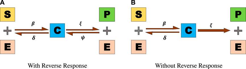
FIGURE 1. Two-step reversible enzymatic reaction. (A) With reverse response. (B) Without reverse response.

For fractional order α, 0 < α ≤ 1, the following chemical reactions can be expressed as a series of fractional differential equations:

$\left\{\begin{array}{c}{}_0{}^{\mathit{CPCF}}\mathrm{D}_t^{\alpha }\mathbf{S}\left(t\right)=\lambda \mathbf{C}-\beta \mathbf{S}\mathbf{E},\hfill \\ {}_0{}^{\mathit{CPCF}}\mathrm{D}_t^{\alpha }\mathbf{E}\left(t\right)=\left(\lambda +\omega \right)\mathbf{C}-\beta \mathbf{S}\mathbf{E},\hfill \\ {}_0{}^{\mathit{CPCF}}\mathrm{D}_t^{\alpha }\mathbf{C}\left(t\right)=\beta \mathbf{S}\mathbf{E}-\left(\lambda +\omega \right)\mathbf{C},\hfill \\ {}_0{}^{\mathit{CPCF}}\mathrm{D}_t^{\alpha }\mathbf{P}\left(t\right)=\omega \mathbf{C}.\hfill \end{array}\right.(1)$

With non-negative initial conditions:

$\mathbf{S}\left(0\right)={\mathbf{S}}_0\ge 0,\mathbf{E}\left(0\right)={\mathbf{E}}_0\ge 0,\mathbf{C}\left(0\right)={\mathbf{C}}_0\ge 0,\mathbf{P}\left(0\right)={\mathbf{P}}_0\ge 0.(2)$

Each of the parameters is considered to be positive for biological consideration. The two-step reversible enzyme reaction model using the CPABC operator is demonstrated as follows:

$\left\{\begin{array}{c}{}_0{}^{\mathit{CPABC}}\mathrm{D}_t^{\alpha }\mathbf{S}\left(t\right)=\lambda \mathbf{C}-\beta \mathbf{S}\mathbf{E},\hfill \\ {}_0{}^{\mathit{CPABC}}\mathrm{D}_t^{\alpha }\mathbf{E}\left(t\right)=\left(\lambda +\omega \right)\mathbf{C}-\beta \mathbf{S}\mathbf{E},\hfill \\ {}_0{}^{\mathit{CPABC}}\mathrm{D}_t^{\alpha }\mathbf{C}\left(t\right)=\beta \mathbf{S}\mathbf{E}-\left(\lambda +\omega \right)\mathbf{C},\hfill \\ {}_0{}^{\mathit{CPABC}}\mathrm{D}_t^{\alpha }\mathbf{P}\left(t\right)=\omega \mathbf{C}.\hfill \end{array}\right.(3)$

Khan et al. [3] stated that the reaction speed of the current chemical process is as follows:

$\mathbf{V}=\frac{\beta \omega e_0\mathbf{S}}{\lambda +\beta \mathbf{S}}.(4)$

This equation can also be re-written as follows:

$\mathbf{V}=\frac{\beta {\mathbb{V}}_{\max }\mathbf{S}}{\lambda +\beta \mathbf{S}}.(5)$

The maximum reaction speed is ${\mathbb{V}}_{\max }=e_0$ when the enzyme and substrate complex has formed.

2.1 Preliminaries

Definition 2.1. The Caputo derivative of a differentiable function G(t) of order α ∈ (0, 1) with the starting point t = 0 is defined as follows [47]:

${}^{C}D_t^{\alpha }\mathrm{G}\left(t\right)=\frac{1}{\mathrm{\Gamma }\left(1-\alpha \right)}{\int }_0^t{\mathrm{G}}^{\prime }\left(\varphi \right){\left(t-\varphi \right)}^{-\alpha }d\varphi .(6)$

Definition 2.2. The Riemann–Liouville (RL) integral [47] is defined using the following formula, assuming that G(t) is an integrable function with 0 < α < 1:

${}^{RL}D_t^{\alpha }\mathrm{G}\left(t\right)=\frac{1}{\mathrm{\Gamma }\left(\alpha \right)}{\int }_0^t{\left(t-\varphi \right)}^{\alpha -1}\mathrm{G}\left(\varphi \right)d\varphi .(7)$

Definition 2.3. The differential operator derived from [48] that may be expressed as a general proportional or conformable operator is defined as follows:

${}^{P}D_t^{\alpha }\mathrm{G}\left(t\right)={\mathrm{Z}}_1\left(\alpha ,t\right)\mathrm{G}\left(t\right)+{\mathrm{Z}}_0\left(\alpha ,t\right){\mathrm{G}}^{\prime }\left(t\right),(8)$

where α ∈ [0, 1]. Z₁ and Z₀ are functions of t that ensure the subsequent criterion $\forall t\in \mathbb{R}$:

$\begin{array}{ll}\hfill & {\displaystyle \underset{\alpha \to 0^{+}}{\lim }}{\mathrm{Z}}_0\left(\alpha ,t\right)=0;{\displaystyle \underset{\alpha \to 1^{-}}{\lim }}{\mathrm{Z}}_0\left(\alpha ,t\right)=1;{\mathrm{Z}}_0\left(\alpha ,t\right)\ne 0,\alpha \in \left(\mathrm{0,1}\right];\hfill \\ \hfill & {\displaystyle \underset{\alpha \to 0^{+}}{\lim }}{\mathrm{Z}}_1\left(\alpha ,t\right)=1;{\displaystyle \underset{\alpha \to 1^{-}}{\lim }}{\mathrm{Z}}_1\left(\alpha ,t\right)=0;{\mathrm{Z}}_1\left(\alpha ,t\right)\ne 0,\alpha \in \left[\mathrm{0,1}\right).\hfill \end{array}(9)$

Consider this operator a generalization of the common differentiation operator (DG(t) = G′(t)), which depends on α. We are also interested in the constant proportionate, or CP, of the specific scenario:

${}^{CP}D_t^{\alpha }\mathrm{G}\left(t\right)={\mathrm{Z}}_1\left(\alpha \right)\mathrm{G}\left(t\right)+{\mathrm{Z}}_0\left(\alpha \right){\mathrm{G}}^{\prime }\left(t\right).(10)$

Definition 2.1. Let 0 < α < 1 and $\mathrm{G}\in {\mathbb{H}}^1(0,\mathrm{T})$, $\mathrm{T}\in {\mathbb{R}}^{+}$. The Caputo–Fabrizio derivative of order α of an integrable function G(t) is indicated by CF and is defined [49] as

${}^{CF}\mathrm{D}_{0,t}^{\alpha }\mathrm{G}\left(t\right)=\frac{\mathrm{M}\left(\alpha \right)}{1-\alpha }{\int }_0^t{\mathrm{G}}^{\prime }\left(\varphi \right)\exp \left[-\frac{\alpha }{1-\alpha }\left(t-\varphi \right)\right]d\varphi ,(11)$

where ${\mathbb{H}}^1(0,\mathrm{T})$ denotes the Sobolev space and M(α), M(0) = M(1) = 1, is a normalization function.

Definition 2.2. Let α ∈ [0, 1] and $\mathrm{G}\in {\mathbb{H}}^1(0,\mathrm{T})$, 0 < T. The Atangana–Baleanu derivative in the Caputo sense of order α of an integrable function G(t) is represented by ABC and is stated as follows [50]:

${}^{\mathit{ABC}}\mathrm{D}_{0,t}^{\alpha }\mathrm{G}\left(t\right)=\frac{\mathrm{A}\mathrm{B}\left(\alpha \right)}{1-\alpha }{\int }_0^t{\mathrm{G}}^{\prime }\left(\varphi \right){\mathrm{E}}_{\alpha }\left[-\frac{\alpha }{1-\alpha }{\left(t-\varphi \right)}^{\alpha }\right]d\varphi ,(12)$

where ${\mathbb{H}}^1(0,\mathrm{T})$ represents the Sobolev space and $\mathrm{A}\mathrm{B}(\alpha )=1-\alpha +\frac{\alpha }{\mathrm{\Gamma }(\alpha )}$ is a normalization function in which AB(0) = AB(1) = 1.

Definition 2.3. The CP (10) and ABC (12) operators are combined to generate CPABC, a novel hybrid fractional operator. It is defined in [37] as follows:

$\begin{array}{cc}\hfill {}_0{}^{\mathit{CPABC}}\mathrm{D}_t^{\alpha }& \mathrm{G}\left(t\right)=\frac{\mathrm{A}\mathrm{B}\left(\alpha \right)}{1-\alpha }{\int }_0^t\left[{\mathrm{Z}}_1\left(\alpha \right)\mathrm{G}\left(\varphi \right)+{\mathrm{Z}}_0\left(\alpha \right){\mathrm{G}}^{\prime }\left(\varphi \right)\right]\exp \left[-\frac{\alpha }{1-\alpha }\left(t-\varphi \right)\right]d\varphi \hfill \\ \hfill & =\frac{\mathrm{A}\mathrm{B}\left(\alpha \right){\mathrm{Z}}_1\left(\alpha \right)}{1-\alpha }{\int }_0^t\mathrm{G}\left(\varphi \right){\mathrm{E}}_{\alpha }\left[-\frac{\alpha }{1-\alpha }{\left(t-\varphi \right)}^{\alpha }\right]d\varphi \hfill \\ \hfill & +\frac{\mathrm{A}\mathrm{B}\left(\alpha \right){\mathrm{Z}}_0\left(\alpha \right)}{1-\alpha }{\int }_0^t{\mathrm{G}}^{\prime }\left(\varphi \right){\mathrm{E}}_{\alpha }\left[-\frac{\alpha }{1-\alpha }{\left(t-\varphi \right)}^{\alpha }\right]d\varphi \hfill \\ \hfill & =\mathrm{G}\left(t\right)\cdot \frac{\mathrm{A}\mathrm{B}\left(\alpha \right){\mathrm{Z}}_1\left(\alpha \right)}{1-\alpha }{\mathrm{E}}_{\alpha }\left(-\frac{\alpha }{1-\alpha }{t}^{\alpha }\right)+{\mathrm{G}}^{\prime }\left(t\right)\cdot \frac{\mathrm{A}\mathrm{B}\left(\alpha \right){\mathrm{Z}}_0\left(\alpha \right)}{1-\alpha }{\mathrm{E}}_{\alpha }\left(-\frac{\alpha }{1-\alpha }{t}^{\alpha }\right).\hfill \end{array}(13)$

Definition 2.4. CPCF, a new hybrid fractional operator formed by combining the CP (10) and CF (11) operators, is defined in [37] as follows:

$\begin{array}{cc}\hfill {}_0{}^{\mathit{CPCF}}\mathrm{D}_t^{\alpha }& \mathrm{G}\left(t\right)=\frac{\mathrm{M}\left(\alpha \right)}{1-\alpha }{\int }_0^t\left[{\mathrm{Z}}_1\left(\alpha \right)\mathrm{G}\left(\varphi \right)+{\mathrm{Z}}_0\left(\alpha \right){\mathrm{G}}^{\prime }\left(\varphi \right)\right]\exp \left(-\frac{\alpha }{1-\alpha }\left(t-\varphi \right)\right)d\varphi \hfill \\ \hfill & =\frac{\mathrm{M}\left(\alpha \right){\mathrm{Z}}_1\left(\alpha \right)}{1-\alpha }{\int }_0^t\mathrm{G}\left(\varphi \right)\exp \left[-\frac{\alpha }{1-\alpha }\left(t-\varphi \right)\right]d\varphi \hfill \\ \hfill & +\frac{\mathrm{M}\left(\alpha \right){\mathrm{Z}}_0\left(\alpha \right)}{1-\alpha }{\int }_0^t{\mathrm{G}}^{\prime }\left(\varphi \right)\exp \left[-\frac{\alpha }{1-\alpha }\left(t-\varphi \right)\right]d\varphi \hfill \\ \hfill & =\mathrm{G}\left(t\right)\cdot \frac{\mathrm{M}\left(\alpha \right){\mathrm{Z}}_1\left(\alpha \right)}{1-\alpha }\exp \left(-\frac{\alpha }{1-\alpha }t\right)+{\mathrm{G}}^{\prime }\left(t\right)\cdot \frac{\mathrm{M}\left(\alpha \right){\mathrm{Z}}_0\left(\alpha \right)}{1-\alpha }\exp \left(-\frac{\alpha }{1-\alpha }t\right).\hfill \end{array}(14)$

3 Analysis of the proposed Model

3.1 Non-negative bounded solutions

The boundedness of the solution for the system (Eq. 1) can be explained by the following equations:

${}_0{}^{\mathit{CPCF}}\mathrm{D}_t^{\alpha }\mathbf{N}\left(t\right)={}_0{}^{\mathit{CPCF}}\mathrm{D}_t^{\alpha }\mathbf{S}\left(t\right)+{}_0{}^{\mathit{CPCF}}\mathrm{D}_t^{\alpha }\mathbf{E}\left(t\right)+{}_0{}^{\mathit{CPCF}}\mathrm{D}_t^{\alpha }\mathbf{C}\left(t\right)+{}_0{}^{\mathit{CPCF}}\mathrm{D}_t^{\alpha }\mathbf{P}\left(t\right).(15)$

Then,

${}_0{}^{\mathit{CPCF}}\mathrm{D}_t^{\alpha }\mathbf{N}\left(t\right)=0,0\le \mathbf{N}\left(0\right)=\mathrm{M},(16)$

where N is the aggregate number of variables included in the proposed system and M is a constant. We have

$\mathbf{N}\left(t\right)\ge \mathrm{M}{e}^{\left(-\frac{{\mathrm{Z}}_1\left(\alpha \right)}{{\mathrm{Z}}_0\left(\alpha \right)}\right)}.(17)$

This implies 0 ≤ N(t) as t → ∞.

⇒ The solutions of the system (Eq. 1) are bounded.

Theorem 3.1. All of the proposed system’s solutions for t ≥ 0 are non-negative under the initial conditions (Eq. 2).

Proof. We have

$\begin{array}{c}{}_0{}^{\mathit{CPCF}}\mathrm{D}_t^{\alpha }{\left.\mathbf{S}\left(t\right)\right|}_{\mathbf{S}=0}=\lambda \mathbf{C}\ge 0,\hfill \\ {}_0{}^{\mathit{CPCF}}\mathrm{D}_t^{\alpha }{\left.\mathbf{E}\left(t\right)\right|}_{\mathbf{E}=0}=\left(\lambda +\omega \right)\mathbf{C}\ge 0,\hfill \\ {}_0{}^{\mathit{CPCF}}\mathrm{D}_t^{\alpha }{\left.\mathbf{C}\left(t\right)\right|}_{\mathbf{C}=0}=\beta \mathbf{S}\mathbf{E}\ge 0,\hfill \\ {}_0{}^{\mathit{CPCF}}\mathrm{D}_t^{\alpha }{\left.\mathbf{P}\left(t\right)\right|}_{\mathbf{P}=0}=\omega \mathbf{C}\ge 0.\hfill \end{array}(18)$

The vector field is considered to be located in the region ${\mathbb{R}}_{+}^4$ on each hyperplane encompassing the non-negative orthant with t ≥ 0, according to system (Eq. 2). Consequently, we identify the area of proposed model (Eq. 2) that is feasible in nature:

$\mathrm{\Delta }=\left\{\left(\mathbf{S},\mathbf{E},\mathbf{C},\mathbf{P}\right)\in {\mathbb{R}}_{+}^4:\mathbf{S}\left(t\right)+\mathbf{E}\left(t\right)+\mathbf{C}\left(t\right)+\mathbf{P}\left(t\right)=\mathbf{N}\left(t\right)\ge 0\right\}.(19)$

3.2 Existence and uniqueness analysis

The validity of the equational framework that ensures the survival of fractional calculus is examined in this section. The following theorem must be proved in order to accomplish this.

Theorem 3.2. Assume that there exist positive constants, χ_q and ${\bar{\chi }}_q$, such that

1. $|{\mathrm{H}}_q(y_q,t)-{\mathrm{H}}_q(y_q^{\prime },t)|\le {\chi }_q|y_q-y_q^{\prime }|,q=\mathrm{1,2,3,4}.$

2. $|{\mathrm{H}}_q(y_q,t){|}^2\le \overline{{\chi }_q}(1+|y_q|),\forall (y,t)\in {\mathbb{R}}^4\times [0,\mathbf{T}].$

Proof. Recalling our model, we obtain

$\left\{\begin{array}{c}{}_0{}^{\mathit{CPCF}}\mathrm{D}_t^{\alpha }\mathbf{S}\left(t\right)=\lambda \mathbf{C}-\beta \mathbf{S}\mathbf{E},\hfill \\ {}_0{}^{\mathit{CPCF}}\mathrm{D}_t^{\alpha }\mathbf{E}\left(t\right)=\left(\lambda +\omega \right)\mathbf{C}-\beta \mathbf{S}\mathbf{E},\hfill \\ {}_0{}^{\mathit{CPCF}}\mathrm{D}_t^{\alpha }\mathbf{C}\left(t\right)=\beta \mathbf{S}\mathbf{E}-\left(\lambda +\omega \right)\mathbf{C},\hfill \\ {}_0{}^{\mathit{CPCF}}\mathrm{D}_t^{\alpha }\mathbf{P}\left(t\right)=\omega \mathbf{C}.\hfill \end{array}\right.(20)$

In order to simplify things, we will present the system as follows:

$\left\{\begin{array}{c}{\mathrm{H}}_1\left(t,\mathbf{S},\mathbf{E},\mathbf{C},\mathbf{P}\right)=\lambda \mathbf{C}-\beta \mathbf{S}\mathbf{E},\hfill \\ {\mathrm{H}}_2\left(t,\mathbf{S},\mathbf{E},\mathbf{C},\mathbf{P}\right)=\left(\lambda +\omega \right)\mathbf{C}-\beta \mathbf{S}\mathbf{E},\hfill \\ {\mathrm{H}}_3\left(t,\mathbf{S},\mathbf{E},\mathbf{C},\mathbf{P}\right)=\beta \mathbf{S}\mathbf{E}-\left(\lambda +\omega \right)\mathbf{C},\hfill \\ {\mathrm{H}}_4\left(t,\mathbf{S},\mathbf{E},\mathbf{C},\mathbf{P}\right)=\omega \mathbf{C}.\hfill \end{array}\right.(21)$

We begin with the function H₁ (t, S, E, C, P). Then, we will show that

${\left|{\mathrm{H}}_1\left(t,{\mathbf{S}}_1,\mathbf{E},\mathbf{C},\mathbf{P}\right)-{\mathrm{H}}_1\left(t,{\mathbf{S}}_2,\mathbf{E},\mathbf{C},\mathbf{P}\right)\right|}^2\le {\chi }_1{\left|{\mathbf{S}}_1-{\mathbf{S}}_2\right|}^2.(22)$

Then, we write

$\left\{\begin{array}{c}{\left|{\mathrm{H}}_1\left(t,{\mathbf{S}}_1,\mathbf{E},\mathbf{C},\mathbf{P}\right)-{\mathrm{H}}_1\left(t,{\mathbf{S}}_2,\mathbf{E},\mathbf{C},\mathbf{P}\right)\right|}^2={\left|-\beta \mathbf{E}\left({\mathbf{S}}_1-{\mathbf{S}}_2\right)\right|}^2\hfill \\ {\left|{\mathrm{H}}_1\left(t,{\mathbf{S}}_1,\mathbf{E},\mathbf{C},\mathbf{P}\right)-{\mathrm{H}}_1\left(t,{\mathbf{S}}_2,\mathbf{E},\mathbf{C},\mathbf{P}\right)\right|}^2={\left|\beta \mathbf{E}\left({\mathbf{S}}_1-{\mathbf{S}}_2\right)\right|}^2\hfill \\ {\left|{\mathrm{H}}_1\left(t,{\mathbf{S}}_1,\mathbf{E},\mathbf{C},\mathbf{P}\right)-{\mathrm{H}}_1\left(t,{\mathbf{S}}_2,\mathbf{E},\mathbf{C},\mathbf{P}\right)\right|}^2\le \left\{2{\beta }^2|\mathbf{E}{|}^2\right\}{\left|\left({\mathbf{S}}_1-{\mathbf{S}}_2\right)\right|}^2\hfill \\ {\left|{\mathrm{H}}_1\left(t,{\mathbf{S}}_1,\mathbf{E},\mathbf{C},\mathbf{P}\right)-{\mathrm{H}}_1\left(t,{\mathbf{S}}_2,\mathbf{E},\mathbf{C},\mathbf{P}\right)\right|}^2\le \left\{2{\beta }^2{\sup }_{0\le t\le \mathbf{T}}|\mathbf{E}{|}^2\right\}{\left|\left({\mathbf{S}}_1-{\mathbf{S}}_2\right)\right|}^2\hfill \\ {\left|{\mathrm{H}}_1\left(t,{\mathbf{S}}_1,\mathbf{E},\mathbf{C},\mathbf{P}\right)-{\mathrm{H}}_1\left(t,{\mathbf{S}}_2,\mathbf{E},\mathbf{C},\mathbf{P}\right)\right|}^2\le \left\{2{\beta }^2|\mathbf{E}{|}_{\infty }^2\right\}{\left|\left({\mathbf{S}}_1-{\mathbf{S}}_2\right)\right|}^2\hfill \\ {\left|{\mathrm{H}}_1\left(t,{\mathbf{S}}_1,\mathbf{E},\mathbf{C},\mathbf{P}\right)-{\mathrm{H}}_1\left(t,{\mathbf{S}}_2,\mathbf{E},\mathbf{C},\mathbf{P}\right)\right|}^2\le {\chi }_1{\left|\left({\mathbf{S}}_1-{\mathbf{S}}_2\right)\right|}^2,\hfill \end{array}\right.(23)$

where ${\chi }_1=2{\beta }^2|\mathbf{E}{|}_{\infty }^2$.

$\left\{\begin{array}{c}{\left|{\mathrm{H}}_2\left(t,\mathbf{S},{\mathbf{E}}_1,\mathbf{C},\mathbf{P}\right)-{\mathrm{H}}_2\left(t,\mathbf{S},{\mathbf{E}}_2,\mathbf{C},\mathbf{P}\right)\right|}^2={\left|-\beta \mathbf{S}\left({\mathbf{E}}_1-{\mathbf{E}}_2\right)\right|}^2\hfill \\ {\left|{\mathrm{H}}_2\left(t,\mathbf{S},{\mathbf{E}}_1,\mathbf{C},\mathbf{P}\right)-{\mathrm{H}}_2\left(t,\mathbf{S},{\mathbf{E}}_2,\mathbf{C},\mathbf{P}\right)\right|}^2={\left|\beta \mathbf{S}\left({\mathbf{E}}_1-{\mathbf{E}}_2\right)\right|}^2\hfill \\ {\left|{\mathrm{H}}_2\left(t,\mathbf{S},{\mathbf{E}}_1,\mathbf{C},\mathbf{P}\right)-{\mathrm{H}}_2\left(t,\mathbf{S},{\mathbf{E}}_2,\mathbf{C},\mathbf{P}\right)\right|}^2\le \left\{2{\beta }^2|\mathbf{S}{|}^2\right\}{\left|\left({\mathbf{E}}_1-{\mathbf{E}}_2\right)\right|}^2\hfill \\ {\left|{\mathrm{H}}_2\left(t,\mathbf{S},{\mathbf{E}}_1,\mathbf{C},\mathbf{P}\right)-{\mathrm{H}}_2\left(t,\mathbf{S},{\mathbf{E}}_2,\mathbf{C},\mathbf{P}\right)\right|}^2\le \left\{2{\beta }^2{\sup }_{0\le t\le \mathbf{T}}|\mathbf{S}{|}^2\right\}{\left|\left({\mathbf{E}}_1-{\mathbf{E}}_2\right)\right|}^2\hfill \\ {\left|{\mathrm{H}}_2\left(t,\mathbf{S},{\mathbf{E}}_1,\mathbf{C},\mathbf{P}\right)-{\mathrm{H}}_2\left(t,\mathbf{S},{\mathbf{E}}_2,\mathbf{C},\mathbf{P}\right)\right|}^2\le \left\{2{\beta }^2|\mathbf{S}{|}_{\infty }^2\right\}{\left|\left({\mathbf{E}}_1-{\mathbf{E}}_2\right)\right|}^2\hfill \\ {\left|{\mathrm{H}}_2\left(t,\mathbf{S},{\mathbf{E}}_1,\mathbf{C},\mathbf{P}\right)-{\mathrm{H}}_2\left(t,\mathbf{S},{\mathbf{E}}_2,\mathbf{C},\mathbf{P}\right)\right|}^2\le {\chi }_2{\left|\left({\mathbf{E}}_1-{\mathbf{E}}_2\right)\right|}^2,\hfill \end{array}\right.(24)$

where ${\chi }_2=2{\beta }^2|\mathbf{S}{|}_{\infty }^2$.

$\left\{\begin{array}{c}{\left|{\mathrm{H}}_3\left(t,\mathbf{S},\mathbf{E},{\mathbf{C}}_1,\mathbf{P}\right)-{\mathrm{H}}_3\left(t,\mathbf{S},\mathbf{E},{\mathbf{C}}_2,\mathbf{P}\right)\right|}^2={\left|-\left(\lambda +\omega \right)\left({\mathbf{C}}_1-{\mathbf{C}}_2\right)\right|}^2\hfill \\ {\left|{\mathrm{H}}_3\left(t,\mathbf{S},\mathbf{E},{\mathbf{C}}_1,\mathbf{P}\right)-{\mathrm{H}}_3\left(t,\mathbf{S},\mathbf{E},{\mathbf{C}}_2,\mathbf{P}\right)\right|}^2={\left|\left(\lambda +\omega \right)\left({\mathbf{C}}_1-{\mathbf{C}}_2\right)\right|}^2\hfill \\ {\left|{\mathrm{H}}_3\left(t,\mathbf{S},\mathbf{E},{\mathbf{C}}_1,\mathbf{P}\right)-{\mathrm{H}}_3\left(t,\mathbf{S},\mathbf{E},{\mathbf{C}}_2,\mathbf{P}\right)\right|}^2\le \left\{2{\lambda }^2+2{\omega }^2\right\}{\left|\left({\mathbf{C}}_1-{\mathbf{C}}_2\right)\right|}^2\hfill \\ {\left|{\mathrm{H}}_3\left(t,\mathbf{S},\mathbf{E},{\mathbf{C}}_1,\mathbf{P}\right)-{\mathrm{H}}_3\left(t,\mathbf{S},\mathbf{E},{\mathbf{C}}_2,\mathbf{P}\right)\right|}^2\le {\chi }_3{\left|\left({\mathbf{C}}_1-{\mathbf{C}}_2\right)\right|}^2,\hfill \end{array}\right.(25)$

where χ₃ = 2λ² + 2ω².

$\left\{\begin{array}{c}{\left|{\mathrm{H}}_4\left(t,\mathbf{S},\mathbf{E},\mathbf{C},{\mathbf{P}}_1\right)-{\mathrm{H}}_4\left(t,\mathbf{S},\mathbf{E},\mathbf{C},{\mathbf{P}}_2\right)\right|}^2=0\hfill \\ {\left|{\mathrm{H}}_4\left(t,\mathbf{S},\mathbf{E},\mathbf{C},{\mathbf{P}}_1\right)-{\mathrm{H}}_4\left(t,\mathbf{S},\mathbf{E},\mathbf{C},{\mathbf{P}}_2\right)\right|}^2\le {\chi }_4{\left|\left({\mathbf{P}}_1-{\mathbf{P}}_2\right)\right|}^2,\hfill \end{array}\right.(26)$

where χ₄ = 0.

The initial condition of each function is double-checked, and then the second requirement of the above theorem will be confirmed:

$\left\{\begin{array}{c}|{\mathrm{H}}_1\left(t,\mathbf{S},\mathbf{E},\mathbf{C},\mathbf{P}\right){|}^2={\left|\lambda \mathbf{C}-\beta \mathbf{S}\mathbf{E}\right|}^2\hfill \\ |{\mathrm{H}}_1\left(t,\mathbf{S},\mathbf{E},\mathbf{C},\mathbf{P}\right){|}^2\le 2{\lambda }^2|\mathbf{C}{|}^2+2{\beta }^2|\mathbf{E}{|}^2|\mathbf{S}{|}^2\hfill \\ |{\mathrm{H}}_1\left(t,\mathbf{S},\mathbf{E},\mathbf{C},\mathbf{P}\right){|}^2\le 2{\lambda }^2{\sup }_{0\le t\le \mathbf{T}}|\mathbf{C}{|}^2+2{\beta }^2{\sup }_{0\le t\le \mathbf{T}}|\mathbf{E}{|}^2{\sup }_{0\le t\le \mathbf{T}}|\mathbf{S}{|}^2\hfill \\ |{\mathrm{H}}_1\left(t,\mathbf{S},\mathbf{E},\mathbf{C},\mathbf{P}\right){|}^2\le 2{\lambda }^2|\mathbf{C}{|}_{\infty }^2+2{\beta }^2|\mathbf{E}{|}_{\infty }^2|\mathbf{S}{|}_{\infty }^2\hfill \\ |{\mathrm{H}}_1\left(t,\mathbf{S},\mathbf{E},\mathbf{C},\mathbf{P}\right){|}^2\le 2\left\{{\lambda }^2|\mathbf{C}{|}_{\infty }^2\right\}\left\{1+\frac{{\beta }^2|\mathbf{E}{|}_{\infty }^2}{{\lambda }^2|\mathbf{C}{|}_{\infty }^2}|\mathbf{S}{|}_{\infty }^2\right\}\hfill \end{array}\right.(27)$

under the condition $\left\{\frac{{\beta }^2|\mathbf{E}{|}_{\infty }^2}{{\lambda }^2|\mathbf{C}{|}_{\infty }^2}\right\}<1$.

$\left\{\begin{array}{c}|{\mathrm{H}}_2\left(t,\mathbf{S},\mathbf{E},\mathbf{C},\mathbf{P}\right){|}^2={\left|\left(\lambda +\omega \right)\mathbf{C}-\beta \mathbf{S}\mathbf{E}\right|}^2\hfill \\ |{\mathrm{H}}_2\left(t,\mathbf{S},\mathbf{E},\mathbf{C},\mathbf{P}\right){|}^2\le \left(2{\lambda }^2+2{\omega }^2\right)|\mathbf{C}{|}^2+2{\beta }^2|\mathbf{S}{|}^2|\mathbf{E}{|}^2\hfill \\ |{\mathrm{H}}_2\left(t,\mathbf{S},\mathbf{E},\mathbf{C},\mathbf{P}\right){|}^2\le \left(2{\lambda }^2+2{\omega }^2\right){\sup }_{0\le t\le \mathbf{T}}|\mathbf{C}{|}^2+2{\beta }^2{\sup }_{0\le t\le \mathbf{T}}|\mathbf{S}{|}^2{\sup }_{0\le t\le \mathbf{T}}|\mathbf{E}{|}^2\hfill \\ |{\mathrm{H}}_2\left(t,\mathbf{S},\mathbf{E},\mathbf{C},\mathbf{P}\right){|}^2\le \left(2{\lambda }^2+2{\omega }^2\right)|\mathbf{C}{|}_{\infty }^2+2{\beta }^2|\mathbf{S}{|}_{\infty }^2|\mathbf{E}{|}_{\infty }^2\hfill \\ |{\mathrm{H}}_2\left(t,\mathbf{S},\mathbf{E},\mathbf{C},\mathbf{P}\right){|}^2\le 2\left\{\left({\lambda }^2+{\omega }^2\right)|\mathbf{C}{|}_{\infty }^2\right\}\left\{1+\frac{{\beta }^2|\mathbf{S}{|}_{\infty }^2}{\left({\lambda }^2+{\omega }^2\right)|\mathbf{C}{|}_{\infty }^2}|\mathbf{E}{|}_{\infty }^2\right\}\hfill \end{array}\right.(28)$

under the condition $\left\{\frac{{\beta }^2|\mathbf{S}{|}_{\infty }^2}{({\lambda }^2+{\omega }^2)|\mathbf{C}{|}_{\infty }^2}\right\}<1$.

$\left\{\begin{array}{c}|{\mathrm{H}}_3\left(t,\mathbf{S},\mathbf{E},\mathbf{C},\mathbf{P}\right){|}^2={\left|\beta \mathbf{S}\mathbf{E}-\left(\lambda +\omega \right)\mathbf{C}\right|}^2\hfill \\ |{\mathrm{H}}_3\left(t,\mathbf{S},\mathbf{E},\mathbf{C},\mathbf{P}\right){|}^2\le 2{\beta }^2|\mathbf{S}{|}^2|\mathbf{E}{|}^2+\left(2{\lambda }^2+2{\omega }^2\right)|\mathbf{C}{|}^2\hfill \\ |{\mathrm{H}}_3\left(t,\mathbf{S},\mathbf{E},\mathbf{C},\mathbf{P}\right){|}^2\le 2{\beta }^2{\sup }_{0\le t\le \mathbf{T}}|\mathbf{S}{|}^2{\sup }_{0\le t\le \mathbf{T}}|\mathbf{E}{|}^2+\left(2{\lambda }^2+2{\omega }^2\right){\sup }_{0\le t\le \mathbf{T}}|\mathbf{C}{|}^2\hfill \\ |{\mathrm{H}}_3\left(t,\mathbf{S},\mathbf{E},\mathbf{C},\mathbf{P}\right){|}^2\le 2{\beta }^2|\mathbf{S}{|}_{\infty }^2|\mathbf{E}{|}_{\infty }^2+2\left({\lambda }^2+{\omega }^2\right)|\mathbf{C}{|}_{\infty }^2\hfill \\ |{\mathrm{H}}_3\left(t,\mathbf{S},\mathbf{E},\mathbf{C},\mathbf{P}\right){|}^2\le 2\left\{{\beta }^2|\mathbf{S}{|}_{\infty }^2|\mathbf{E}{|}_{\infty }^2\right\}\left\{1+\frac{{\lambda }^2+{\omega }^2}{{\beta }^2|\mathbf{S}{|}_{\infty }^2|\mathbf{E}{|}_{\infty }^2}|\mathbf{C}{|}_{\infty }^2\right\}\hfill \end{array}\right.(29)$

under the condition $\left\{\frac{{\lambda }^2+{\omega }^2}{{\beta }^2|\mathbf{S}{|}_{\infty }^2|\mathbf{E}{|}_{\infty }^2}\right\}<1$.

$\left\{\begin{array}{c}|{\mathrm{H}}_4\left(t,\mathbf{S},\mathbf{E},\mathbf{C},\mathbf{P}\right){|}^2={\left|\omega \mathbf{C}\right|}^2\hfill \\ |{\mathrm{H}}_4\left(t,\mathbf{S},\mathbf{E},\mathbf{C},\mathbf{P}\right){|}^2\le 2{\omega }^2|\mathbf{C}{|}^2+2\hfill \\ |{\mathrm{H}}_4\left(t,\mathbf{S},\mathbf{E},\mathbf{C},\mathbf{P}\right){|}^2\le 2{\omega }^2|\mathbf{C}{|}^2\left\{1+\frac{1}{{\omega }^2|\mathbf{C}{|}_{\infty }^4}|\mathbf{C}{|}_{\infty }^2\right\}\hfill \end{array}\right.(30)$

under the condition $\left\{\frac{1}{{\omega }^2|\mathbf{C}{|}_{\infty }^4}\right\}<1$.

As a result, the solution to our system is distinct and appropriate in the given situation:

$Max\left\{\begin{array}{c}\left\{\frac{{\beta }^2|\mathbf{E}{|}_{\infty }^2}{{\lambda }^2|\mathbf{C}{|}_{\infty }^2}\right\},\hfill \\ \left\{\frac{{\beta }^2|\mathbf{S}{|}_{\infty }^2}{\left({\lambda }^2+{\omega }^2\right)|\mathbf{C}{|}_{\infty }^2}\right\},\hfill \\ \left\{\frac{{\lambda }^2+{\omega }^2}{{\beta }^2|\mathbf{S}{|}_{\infty }^2|\mathbf{E}{|}_{\infty }^2}\right\},\hfill \\ \left\{\frac{1}{{\omega }^2|\mathbf{C}{|}_{\infty }^4}\right\}.\hfill \end{array}\right.<1(31)$

3.3 Analysis of the proposed model’s stability

To understand the dynamical properties of the suggested model (Eq. 1), a qualitative study is conducted.

Theorem 3.3. Let V be a self-map on the Banach space $\mathcal{B}$. This implies that the following inequality is true for all instances of V.

$\Vert {\mathrm{V}}_x^{*}-{\mathrm{V}}_y^{*}\Vert \le C\Vert x-{\mathrm{V}}^{*}\Vert +c\Vert x-y\Vert ,(32)$

with e ∈ [0, 1), E ≥ 0, if we suppose that V* is Picard V* stable.

Proof. Let V* be Picard V* stable. Examining the equations associated with the proposed model (Eq. 1), we obtain

$\begin{array}{cc}\hfill {\mathbf{S}}_{j+1}\left(t\right)& ={\mathbf{S}}_j\left(t\right)+{\mathfrak{L}}^{-1}\left[\frac{\alpha +s\left(1-\alpha \right)}{\mathbb{M}\left(\alpha \right){\mathrm{Z}}_1\left(\alpha \right)+s\mathrm{M}\left(\alpha \right){\mathrm{Z}}_0\left(\alpha \right)}\mathfrak{L}\left(\lambda {\mathbf{C}}_j-\beta {\mathbf{S}}_j{\mathbf{E}}_j\right)\right],\hfill \\ \hfill {\mathbf{E}}_{j+1}\left(t\right)& ={\mathbf{E}}_j\left(t\right)+{\mathfrak{L}}^{-1}\left[\frac{\alpha +s\left(1-\alpha \right)}{\mathbb{M}\left(\alpha \right){\mathrm{Z}}_1\left(\alpha \right)+s\mathrm{M}\left(\alpha \right){\mathrm{Z}}_0\left(\alpha \right)}\mathfrak{L}\left(\left(\lambda +\omega \right){\mathbf{C}}_j-\beta {\mathbf{S}}_j{\mathbf{E}}_j\right)\right],\hfill \\ \hfill {\mathbf{C}}_{j+1}\left(t\right)& ={\mathbf{C}}_j\left(t\right)+{\mathfrak{L}}^{-1}\left[\frac{\alpha +s\left(1-\alpha \right)}{\mathbb{M}\left(\alpha \right){\mathrm{Z}}_1\left(\alpha \right)+s\mathrm{M}\left(\alpha \right){\mathrm{Z}}_0\left(\alpha \right)}\mathfrak{L}\left(\beta {\mathbf{S}}_j{\mathbf{E}}_j-\left(\lambda +\omega \right){\mathbf{C}}_j\right)\right],\hfill \\ \hfill {\mathbf{P}}_{j+1}\left(t\right)& ={\mathbf{P}}_j\left(t\right)+{\mathfrak{L}}^{-1}\left[\frac{\alpha +s\left(1-\alpha \right)}{\mathbb{M}\left(\alpha \right){\mathrm{Z}}_1\left(\alpha \right)+s\mathrm{M}\left(\alpha \right){\mathrm{Z}}_0\left(\alpha \right)}\mathfrak{L}\left(\omega {\mathbf{C}}_j\right)\right],\hfill \end{array}(33)$

where $\frac{\alpha +s(1-\alpha )}{\mathbb{M}(\alpha ){\mathrm{Z}}_1(\alpha )+s\mathrm{M}(\alpha ){\mathrm{Z}}_0(\alpha )}$ represents the fractional Lagrange multiplier.

Theorem 3.4. Let a self-map $\mathbb{Q}$ defined as

$\begin{array}{cc}\hfill \mathbb{Q}\left[{\mathbf{S}}_j\right]={\mathbf{S}}_{j+1}\left(t\right)& ={\mathbf{S}}_j\left(t\right)+{\mathfrak{L}}^{-1}\left[\frac{\alpha +s\left(1-\alpha \right)}{\mathbb{M}\left(\alpha \right){\mathrm{Z}}_1\left(\alpha \right)+s\mathrm{M}\left(\alpha \right){\mathrm{Z}}_0\left(\alpha \right)}\mathfrak{L}\left(\lambda {\mathbf{C}}_j-\beta {\mathbf{S}}_j{\mathbf{E}}_j\right)\right],\hfill \\ \hfill \mathbb{Q}\left[{\mathbf{E}}_j\right]={\mathbf{E}}_{j+1}\left(t\right)& ={\mathbf{E}}_j\left(t\right)+{\mathfrak{L}}^{-1}\left[\frac{\alpha +s\left(1-\alpha \right)}{\mathbb{M}\left(\alpha \right){\mathrm{Z}}_1\left(\alpha \right)+s\mathrm{M}\left(\alpha \right){\mathrm{Z}}_0\left(\alpha \right)}\mathfrak{L}\left(\left(\lambda +\omega \right){\mathbf{C}}_j-\beta {\mathbf{S}}_j{\mathbf{E}}_j\right)\right],\hfill \\ \hfill \mathbb{Q}\left[{\mathbf{C}}_j\right]={\mathbf{C}}_{j+1}\left(t\right)& ={\mathbf{C}}_j\left(t\right)+{\mathfrak{L}}^{-1}\left[\frac{\alpha +s\left(1-\alpha \right)}{\mathbb{M}\left(\alpha \right){\mathrm{Z}}_1\left(\alpha \right)+s\mathrm{M}\left(\alpha \right){\mathrm{Z}}_0\left(\alpha \right)}\mathfrak{L}\left(\beta {\mathbf{S}}_j{\mathbf{E}}_j-\left(\lambda +\omega \right){\mathbf{C}}_j\right)\right],\hfill \\ \hfill \mathbb{Q}\left[{\mathbf{P}}_j\right]={\mathbf{P}}_{j+1}\left(t\right)& ={\mathbf{P}}_j\left(t\right)+{\mathfrak{L}}^{-1}\left[\frac{\alpha +s\left(1-\alpha \right)}{\mathbb{M}\left(\alpha \right){\mathrm{Z}}_1\left(\alpha \right)+s\mathrm{M}\left(\alpha \right){\mathrm{Z}}_0\left(\alpha \right)}\mathfrak{L}\left(\omega {\mathbf{C}}_j\right)\right]\hfill \end{array}(34)$

be V* stable in the space of L¹ (a, b) if

$\mathrm{\Psi }=\left\{\begin{array}{c}\left\{1+\lambda {\phi }_1\left(\alpha \right)+\beta {\mathrm{\Theta }}_1{\phi }_2\left(\alpha \right)+\beta {\mathrm{\Theta }}_2{\phi }_3\left(\alpha \right)\right\}<1,\hfill \\ \left\{1+\left(\lambda +\omega \right){\phi }_4\left(\alpha \right)+\beta {\mathrm{\Theta }}_1{\phi }_5\left(\alpha \right)+\beta {\mathrm{\Theta }}_2{\phi }_6\left(\alpha \right)\right\}<1,\hfill \\ \left\{1+\beta {\mathrm{\Theta }}_1{\phi }_7\left(\alpha \right)+\beta {\mathrm{\Theta }}_2{\phi }_8\left(\alpha \right)+\left(\lambda +\omega \right){\phi }_9\left(\alpha \right)\right\}<1,\hfill \\ \left\{1+\omega {\phi }_{10}\left(\alpha \right)\right\}<1.\hfill \end{array}\right.(35)$

Proof. Given that $\mathbb{Q}$ is a fixed point, one can find $(m,n)\in (\mathbb{N}\times \mathbb{N})$ Â for each

$\left\{\begin{array}{c}\mathbb{Q}\left[{\mathbf{S}}_y\right]-\mathbb{Q}\left[{\mathbf{S}}_x\right]={\mathbf{S}}_{j+1}\left(t\right)={\mathbf{S}}_y\left(t\right)+{\mathfrak{L}}^{-1}\left[\frac{\alpha +s\left(1-\alpha \right)}{\mathbb{M}\left(\alpha \right){\mathrm{Z}}_1\left(\alpha \right)+s\mathrm{M}\left(\alpha \right){\mathrm{Z}}_0\left(\alpha \right)}\mathfrak{L}\left(\lambda {\mathbf{C}}_y-\beta {\mathbf{S}}_y{\mathbf{E}}_y\right)\right]\hfill \\ -{\mathbf{S}}_x\left(t\right)-{\mathfrak{L}}^{-1}\left[\frac{\alpha +s\left(1-\alpha \right)}{\mathbb{M}\left(\alpha \right){\mathrm{Z}}_1\left(\alpha \right)+s\mathrm{M}\left(\alpha \right){\mathrm{Z}}_0\left(\alpha \right)}\mathfrak{L}\left(\lambda {\mathbf{C}}_x-\beta {\mathbf{S}}_x{\mathbf{E}}_x\right)\right],\hfill \\ \mathbb{Q}\left[{\mathbf{E}}_y\right]-\mathbb{Q}\left[{\mathbf{E}}_x\right]={\mathbf{E}}_{j+1}\left(t\right)={\mathbf{E}}_y\left(t\right)+{\mathfrak{L}}^{-1}\left[\frac{\alpha +s\left(1-\alpha \right)}{\mathbb{M}\left(\alpha \right){\mathrm{Z}}_1\left(\alpha \right)+s\mathrm{M}\left(\alpha \right){\mathrm{Z}}_0\left(\alpha \right)}\mathfrak{L}\left(\left(\lambda +\omega \right){\mathbf{C}}_y-\beta {\mathbf{S}}_y{\mathbf{E}}_y\right)\right]\hfill \\ -{\mathbf{E}}_x\left(t\right)-{\mathfrak{L}}^{-1}\left[\frac{\alpha +s\left(1-\alpha \right)}{\mathbb{M}\left(\alpha \right){\mathrm{Z}}_1\left(\alpha \right)+s\mathrm{M}\left(\alpha \right){\mathrm{Z}}_0\left(\alpha \right)}\mathfrak{L}\left(\left(\lambda +\omega \right){\mathbf{C}}_x-\beta {\mathbf{S}}_x{\mathbf{E}}_x\right)\right],\hfill \\ \mathbb{Q}\left[{\mathbf{C}}_y\right]-\mathbb{Q}\left[{\mathbf{C}}_x\right]={\mathbf{C}}_{j+1}\left(t\right)={\mathbf{C}}_y\left(t\right)+{\mathfrak{L}}^{-1}\left[\frac{\alpha +s\left(1-\alpha \right)}{\mathbb{M}\left(\alpha \right){\mathrm{Z}}_1\left(\alpha \right)+s\mathrm{M}\left(\alpha \right){\mathrm{Z}}_0\left(\alpha \right)}\mathfrak{L}\left(\beta {\mathbf{S}}_y{\mathbf{E}}_y-\left(\lambda +\omega \right){\mathbf{C}}_y\right)\right]\hfill \\ -{\mathbf{C}}_x\left(t\right)-{\mathfrak{L}}^{-1}\left[\frac{\alpha +s\left(1-\alpha \right)}{\mathbb{M}\left(\alpha \right){\mathrm{Z}}_1\left(\alpha \right)+s\mathrm{M}\left(\alpha \right){\mathrm{Z}}_0\left(\alpha \right)}\mathfrak{L}\left(\beta {\mathbf{S}}_x{\mathbf{E}}_x-\left(\lambda +\omega \right){\mathbf{C}}_x\right)\right],\hfill \\ \mathbb{Q}\left[{\mathbf{P}}_y\right]-\mathbb{Q}\left[{\mathbf{P}}_x\right]={\mathbf{P}}_{j+1}\left(t\right)={\mathbf{P}}_y\left(t\right)+{\mathfrak{L}}^{-1}\left[\frac{\alpha +s\left(1-\alpha \right)}{\mathbb{M}\left(\alpha \right){\mathrm{Z}}_1\left(\alpha \right)+s\mathrm{M}\left(\alpha \right){\mathrm{Z}}_0\left(\alpha \right)}\mathfrak{L}\left(\omega {\mathbf{C}}_y\right)\right]\hfill \\ -{\mathbf{P}}_x\left(t\right)-{\mathfrak{L}}^{-1}\left[\frac{\alpha +s\left(1-\alpha \right)}{\mathbb{M}\left(\alpha \right){\mathrm{Z}}_1\left(\alpha \right)+s\mathrm{M}\left(\alpha \right){\mathrm{Z}}_0\left(\alpha \right)}\mathfrak{L}\left(\omega {\mathbf{C}}_x\right)\right].\hfill \end{array}\right.(36)$

Without losing generality and by applying the norm to Eq. 36, we obtain

$\left\{\begin{array}{c}\Vert \mathbb{Q}\left[{\mathbf{S}}_y\right]-\mathbb{Q}\left[{\mathbf{S}}_x\right]\Vert =‖{\mathbf{S}}_y\left(t\right)+{\mathfrak{L}}^{-1}\left[\frac{\alpha +s\left(1-\alpha \right)}{\mathbb{M}\left(\alpha \right){\mathrm{Z}}_1\left(\alpha \right)+s\mathrm{M}\left(\alpha \right){\mathrm{Z}}_0\left(\alpha \right)}\mathfrak{L}\left(\lambda {\mathbf{C}}_y-\beta {\mathbf{S}}_y{\mathbf{E}}_y\right)\right]\hfill \\ -{\mathbf{S}}_x\left(t\right)-{\mathfrak{L}}^{-1}\left[\frac{\alpha +s\left(1-\alpha \right)}{\mathbb{M}\left(\alpha \right){\mathrm{Z}}_1\left(\alpha \right)+s\mathrm{M}\left(\alpha \right){\mathrm{Z}}_0\left(\alpha \right)}\mathfrak{L}\left(\lambda {\mathbf{C}}_x-\beta {\mathbf{S}}_x{\mathbf{E}}_x\right)\right]‖,\hfill \\ \Vert \mathbb{Q}\left[{\mathbf{E}}_y\right]-\mathbb{Q}\left[{\mathbf{E}}_x\right]\Vert =‖{\mathbf{E}}_y\left(t\right)+{\mathfrak{L}}^{-1}\left[\frac{\alpha +s\left(1-\alpha \right)}{\mathbb{M}\left(\alpha \right){\mathrm{Z}}_1\left(\alpha \right)+s\mathrm{M}\left(\alpha \right){\mathrm{Z}}_0\left(\alpha \right)}\mathfrak{L}\left(\left(\lambda +\omega \right){\mathbf{C}}_y-\beta {\mathbf{S}}_y{\mathbf{E}}_y\right)\right]\hfill \\ -{\mathbf{E}}_x\left(t\right)-{\mathfrak{L}}^{-1}\left[\frac{\alpha +s\left(1-\alpha \right)}{\mathbb{M}\left(\alpha \right){\mathrm{Z}}_1\left(\alpha \right)+s\mathrm{M}\left(\alpha \right){\mathrm{Z}}_0\left(\alpha \right)}\mathfrak{L}\left(\left(\lambda +\omega \right){\mathbf{C}}_x-\beta {\mathbf{S}}_x{\mathbf{E}}_x\right)\right]‖,\hfill \\ \Vert \mathbb{Q}\left[{\mathbf{C}}_y\right]-\mathbb{Q}\left[{\mathbf{C}}_x\right]\Vert =‖{\mathbf{C}}_y\left(t\right)+{\mathfrak{L}}^{-1}\left[\frac{\alpha +s\left(1-\alpha \right)}{\mathbb{M}\left(\alpha \right){\mathrm{Z}}_1\left(\alpha \right)+s\mathrm{M}\left(\alpha \right){\mathrm{Z}}_0\left(\alpha \right)}\mathfrak{L}\left(\beta {\mathbf{S}}_y{\mathbf{E}}_y-\left(\lambda +\omega \right){\mathbf{C}}_y\right)\right]\hfill \\ -{\mathbf{C}}_x\left(t\right)-{\mathfrak{L}}^{-1}\left[\frac{\alpha +s\left(1-\alpha \right)}{\mathbb{M}\left(\alpha \right){\mathrm{Z}}_1\left(\alpha \right)+s\mathrm{M}\left(\alpha \right){\mathrm{Z}}_0\left(\alpha \right)}\mathfrak{L}\left(\beta {\mathbf{S}}_x{\mathbf{E}}_x-\left(\lambda +\omega \right){\mathbf{C}}_x\right)\right]‖,\hfill \\ \Vert \mathbb{Q}\left[{\mathbf{P}}_y\right]-\mathbb{Q}\left[{\mathbf{P}}_x\right]\Vert =‖{\mathbf{P}}_y\left(t\right)+{\mathfrak{L}}^{-1}\left[\frac{\alpha +s\left(1-\alpha \right)}{\mathbb{M}\left(\alpha \right){\mathrm{Z}}_1\left(\alpha \right)+s\mathrm{M}\left(\alpha \right){\mathrm{Z}}_0\left(\alpha \right)}\mathfrak{L}\left(\omega {\mathbf{C}}_y\right)\right]\hfill \\ -{\mathbf{P}}_x\left(t\right)-{\mathfrak{L}}^{-1}\left[\frac{\alpha +s\left(1-\alpha \right)}{\mathbb{M}\left(\alpha \right){\mathrm{Z}}_1\left(\alpha \right)+s\mathrm{M}\left(\alpha \right){\mathrm{Z}}_0\left(\alpha \right)}\mathfrak{L}\left(\omega {\mathbf{C}}_x\right)\right]‖.\hfill \end{array}\right.(37)$

After applying triangle inequality, we have

$\left\{\begin{array}{c}\Vert \mathbb{Q}\left[{\mathbf{S}}_y\right]-\mathbb{Q}\left[{\mathbf{S}}_x\right]\Vert \le ‖{\mathbf{S}}_y\left(t\right)-{\mathbf{S}}_y\left(t\right)‖+{\mathfrak{L}}^{-1}\left[\frac{\alpha +s\left(1-\alpha \right)}{\mathbb{M}\left(\alpha \right){\mathrm{Z}}_1\left(\alpha \right)+s\mathrm{M}\left(\alpha \right){\mathrm{Z}}_0\left(\alpha \right)}\mathfrak{L}\left\{\Vert \lambda \left({\mathbf{C}}_y-{\mathbf{C}}_x\right)\Vert \right.\right.\hfill \\ \left.+\Vert \beta {\mathbf{S}}_y\left({\mathbf{E}}_y-{\mathbf{E}}_x\right)\Vert +\Vert \beta {\mathbf{E}}_y\left({\mathbf{S}}_y-{\mathbf{S}}_x\right)\Vert \right\}],\hfill \\ \Vert \mathbb{Q}\left[{\mathbf{E}}_y\right]-\mathbb{Q}\left[{\mathbf{E}}_x\right]\Vert \le ‖{\mathbf{E}}_y\left(t\right)-{\mathbf{E}}_y\left(t\right)‖+{\mathfrak{L}}^{-1}\left[\frac{\alpha +s\left(1-\alpha \right)}{\mathbb{M}\left(\alpha \right){\mathrm{Z}}_1\left(\alpha \right)+s\mathrm{M}\left(\alpha \right){\mathrm{Z}}_0\left(\alpha \right)}\mathfrak{L}\left\{\Vert \left(\lambda +\omega \right)\left({\mathbf{C}}_y-{\mathbf{C}}_x\right)\Vert \right.\right.\hfill \\ +\Vert \beta {\mathbf{S}}_y\left({\mathbf{E}}_y-{\mathbf{E}}_x\right)\Vert \left.+\Vert \beta {\mathbf{E}}_y\left({\mathbf{S}}_y-{\mathbf{S}}_x\right)\Vert \right\}],\hfill \\ \Vert \mathbb{Q}\left[{\mathbf{C}}_y\right]-\mathbb{Q}\left[{\mathbf{C}}_x\right]\Vert \le ‖{\mathbf{C}}_y\left(t\right)-{\mathbf{C}}_y\left(t\right)‖+{\mathfrak{L}}^{-1}\left[\frac{\alpha +s\left(1-\alpha \right)}{\mathbb{M}\left(\alpha \right){\mathrm{Z}}_1\left(\alpha \right)+s\mathrm{M}\left(\alpha \right){\mathrm{Z}}_0\left(\alpha \right)}\mathfrak{L}\left\{\Vert \beta {\mathbf{S}}_y\left({\mathbf{E}}_y-{\mathbf{E}}_x\right)\Vert \right.\right.\hfill \\ +\Vert \beta {\mathbf{E}}_y\left({\mathbf{S}}_y-{\mathbf{S}}_x\right)\Vert \left.+\Vert \left(\lambda +\omega \right)\left({\mathbf{C}}_y-{\mathbf{C}}_x\right)\Vert \right\}],\hfill \\ \Vert \mathbb{Q}\left[{\mathbf{P}}_y\right]-\mathbb{Q}\left[{\mathbf{P}}_x\right]\Vert \le ‖{\mathbf{P}}_y\left(t\right)-{\mathbf{P}}_y\left(t\right)‖+{\mathfrak{L}}^{-1}\left[\frac{\alpha +s\left(1-\alpha \right)}{\mathbb{M}\left(\alpha \right){\mathrm{Z}}_1\left(\alpha \right)+s\mathrm{M}\left(\alpha \right){\mathrm{Z}}_0\left(\alpha \right)}\mathfrak{L}\left\{\Vert \omega \left({\mathbf{C}}_y-{\mathbf{C}}_x\right)\Vert \right\}\right].\hfill \end{array}\right.(38)$

Considering that the solutions found play a similar role, we conclude that

$\Vert {\mathbf{S}}_y\left(t\right)-{\mathbf{S}}_x\left(t\right)\Vert =\Vert {\mathbf{E}}_y\left(t\right)-{\mathbf{E}}_x\left(t\right)\Vert =\Vert {\mathbf{C}}_y\left(t\right)-{\mathbf{C}}_x\left(t\right)\Vert =\Vert {\mathbf{P}}_y\left(t\right)-{\mathbf{P}}_x\left(t\right)\Vert .(39)$

By substituting this into Eq. 38, one can obtain the relationship shown below:

$\left\{\begin{array}{c}\Vert \mathbb{Q}\left[{\mathbf{S}}_y\right]-\mathbb{Q}\left[{\mathbf{S}}_x\right]\Vert \le ‖{\mathbf{S}}_y\left(t\right)-{\mathbf{S}}_y\left(t\right)‖+{\mathfrak{L}}^{-1}\left[\frac{\alpha +s\left(1-\alpha \right)}{\mathbb{M}\left(\alpha \right){\mathrm{Z}}_1\left(\alpha \right)+s\mathrm{M}\left(\alpha \right){\mathrm{Z}}_0\left(\alpha \right)}\mathfrak{L}\left\{\Vert \lambda \left({\mathbf{S}}_y-{\mathbf{S}}_x\right)\Vert \right.\right.\hfill \\ +\Vert \beta {\mathbf{S}}_y\left({\mathbf{S}}_y-{\mathbf{S}}_x\right)\Vert \left.+\Vert \beta {\mathbf{E}}_y\left({\mathbf{S}}_y-{\mathbf{S}}_x\right)\Vert \right\}],\hfill \\ \Vert \mathbb{Q}\left[{\mathbf{E}}_y\right]-\mathbb{Q}\left[{\mathbf{E}}_x\right]\Vert \le ‖{\mathbf{E}}_y\left(t\right)-{\mathbf{E}}_y\left(t\right)‖+{\mathfrak{L}}^{-1}\left[\frac{\alpha +s\left(1-\alpha \right)}{\mathbb{M}\left(\alpha \right){\mathrm{Z}}_1\left(\alpha \right)+s\mathrm{M}\left(\alpha \right){\mathrm{Z}}_0\left(\alpha \right)}\mathfrak{L}\left\{\Vert \left(\lambda +\omega \right)\left({\mathbf{E}}_y-{\mathbf{E}}_x\right)\Vert \right.\right.\hfill \\ +\Vert \beta {\mathbf{S}}_y\left({\mathbf{E}}_y-{\mathbf{E}}_x\right)\Vert \left.+\Vert \beta {\mathbf{E}}_y\left({\mathbf{E}}_y-{\mathbf{E}}_x\right)\Vert \right\}],\hfill \\ \Vert \mathbb{Q}\left[{\mathbf{C}}_y\right]-\mathbb{Q}\left[{\mathbf{C}}_x\right]\Vert \le ‖{\mathbf{C}}_y\left(t\right)-{\mathbf{C}}_y\left(t\right)‖+{\mathfrak{L}}^{-1}\left[\frac{\alpha +s\left(1-\alpha \right)}{\mathbb{M}\left(\alpha \right){\mathrm{Z}}_1\left(\alpha \right)+s\mathrm{M}\left(\alpha \right){\mathrm{Z}}_0\left(\alpha \right)}\mathfrak{L}\left\{\Vert \beta {\mathbf{S}}_y\left({\mathbf{E}}_y-{\mathbf{E}}_x\right)\Vert \right.\right.\hfill \\ +\Vert \beta {\mathbf{E}}_y\left({\mathbf{C}}_y-{\mathbf{C}}_x\right)\Vert \left.+\Vert \left(\lambda +\omega \right)\left({\mathbf{C}}_y-{\mathbf{C}}_x\right)\Vert \right\}],\hfill \\ \Vert \mathbb{Q}\left[{\mathbf{P}}_y\right]-\mathbb{Q}\left[{\mathbf{P}}_x\right]\Vert \le ‖{\mathbf{P}}_y\left(t\right)-{\mathbf{P}}_y\left(t\right)‖+{\mathfrak{L}}^{-1}\left[\frac{\alpha +s\left(1-\alpha \right)}{\mathbb{M}\left(\alpha \right){\mathrm{Z}}_1\left(\alpha \right)+s\mathrm{M}\left(\alpha \right){\mathrm{Z}}_0\left(\alpha \right)}\mathfrak{L}\left\{\Vert \omega \left({\mathbf{P}}_y-{\mathbf{P}}_x\right)\Vert \right\}\right].\hfill \end{array}\right.(40)$

Simplifying the aforementioned equation, we obtain Eq. 41 as follows:

$\left\{\begin{array}{c}\Vert \mathbb{Q}\left[{\mathbf{S}}_y\right]-\mathbb{Q}\left[{\mathbf{S}}_x\right]\Vert \le ‖{\mathbf{S}}_y\left(t\right)-{\mathbf{S}}_y\left(t\right)‖+{\mathfrak{L}}^{-1}\left[\frac{\alpha +s\left(1-\alpha \right)}{\mathbb{M}\left(\alpha \right){\mathrm{Z}}_1\left(\alpha \right)+s\mathrm{M}\left(\alpha \right){\mathrm{Z}}_0\left(\alpha \right)}\mathfrak{L}\left\{\lambda \Vert \left({\mathbf{S}}_y-{\mathbf{S}}_x\right)\Vert \right.\right.\hfill \\ \left.+\beta \Vert {\mathbf{S}}_y\Vert \Vert \left({\mathbf{S}}_y-{\mathbf{S}}_x\right)\Vert +\beta \Vert {\mathbf{E}}_y\Vert \Vert \left({\mathbf{S}}_y-{\mathbf{S}}_x\right)\Vert \right\}],\hfill \\ \Vert \mathbb{Q}\left[{\mathbf{E}}_y\right]-\mathbb{Q}\left[{\mathbf{E}}_x\right]\Vert \le ‖{\mathbf{E}}_y\left(t\right)-{\mathbf{E}}_y\left(t\right)‖+{\mathfrak{L}}^{-1}\left[\frac{\alpha +s\left(1-\alpha \right)}{\mathbb{M}\left(\alpha \right){\mathrm{Z}}_1\left(\alpha \right)+s\mathrm{M}\left(\alpha \right){\mathrm{Z}}_0\left(\alpha \right)}\mathfrak{L}\left\{\left(\lambda +\omega \right)\Vert \left({\mathbf{E}}_y-{\mathbf{E}}_x\right)\Vert \right.\right.\hfill \\ \left.+\beta \Vert {\mathbf{S}}_y\Vert \Vert \left({\mathbf{E}}_y-{\mathbf{E}}_x\right)\Vert +\beta \Vert {\mathbf{E}}_y\Vert \Vert \left({\mathbf{E}}_y-{\mathbf{E}}_x\right)\Vert \right\}],\hfill \\ \Vert \mathbb{Q}\left[{\mathbf{C}}_y\right]-\mathbb{Q}\left[{\mathbf{C}}_x\right]\Vert \le ‖{\mathbf{C}}_y\left(t\right)-{\mathbf{C}}_y\left(t\right)‖+{\mathfrak{L}}^{-1}\left[\frac{\alpha +s\left(1-\alpha \right)}{\mathbb{M}\left(\alpha \right){\mathrm{Z}}_1\left(\alpha \right)+s\mathrm{M}\left(\alpha \right){\mathrm{Z}}_0\left(\alpha \right)}\mathfrak{L}\left\{\beta \Vert {\mathbf{S}}_y\Vert \Vert \left({\mathbf{E}}_y-{\mathbf{E}}_x\right)\Vert \right.\right.\hfill \\ \left.+\beta \Vert {\mathbf{E}}_y\Vert \Vert \left({\mathbf{C}}_y-{\mathbf{C}}_x\right)\Vert +\left(\lambda +\omega \right)\Vert \left({\mathbf{C}}_y-{\mathbf{C}}_x\right)\Vert \right\}],\hfill \\ \Vert \mathbb{Q}\left[{\mathbf{P}}_y\right]-\mathbb{Q}\left[{\mathbf{P}}_x\right]\Vert \le ‖{\mathbf{P}}_y\left(t\right)-{\mathbf{P}}_y\left(t\right)‖+{\mathfrak{L}}^{-1}\left[\frac{\alpha +s\left(1-\alpha \right)}{\mathbb{M}\left(\alpha \right){\mathrm{Z}}_1\left(\alpha \right)+s\mathrm{M}\left(\alpha \right){\mathrm{Z}}_0\left(\alpha \right)}\mathfrak{L}\left\{\omega \Vert \left({\mathbf{P}}_y-{\mathbf{P}}_x\right)\Vert \right\}\right].\hfill \end{array}\right.(41)$

Additionally, because these are convergent sequences, S_y and E_y are bounded. However, we can obtain alternate positive constants Θ₁ and Θ₂ for every t, such that

$\Vert {\mathbf{S}}_y\Vert <{\mathrm{\Theta }}_1,\Vert {\mathbf{E}}_y\Vert <{\mathrm{\Theta }}_2.(42)$

Hence, we can write

$\left\{\begin{array}{c}\Vert \mathbb{Q}\left[{\mathbf{S}}_y\right]-\mathbb{Q}\left[{\mathbf{S}}_x\right]\Vert \le \left\{1+\lambda {\phi }_1\left(\alpha \right)+\beta {\mathrm{\Theta }}_1{\phi }_2\left(\alpha \right)+\beta {\mathrm{\Theta }}_2{\phi }_3\left(\alpha \right)\right\}\Vert \left({\mathbf{S}}_y-{\mathbf{S}}_x\right)\Vert ,\hfill \\ \Vert \mathbb{Q}\left[{\mathbf{E}}_y\right]-\mathbb{Q}\left[{\mathbf{E}}_x\right]\Vert \le \left\{1+\left(\lambda +\omega \right){\phi }_4\left(\alpha \right)+\beta {\mathrm{\Theta }}_1{\phi }_5\left(\alpha \right)+\beta {\mathrm{\Theta }}_2{\phi }_6\left(\alpha \right)\right\}\Vert \left({\mathbf{E}}_y-{\mathbf{E}}_x\right)\Vert ,\hfill \\ \Vert \mathbb{Q}\left[{\mathbf{C}}_y\right]-\mathbb{Q}\left[{\mathbf{C}}_x\right]\Vert \le \left\{1+\beta {\mathrm{\Theta }}_1{\phi }_7\left(\alpha \right)+\beta {\mathrm{\Theta }}_2{\phi }_8\left(\alpha \right)+\left(\lambda +\omega \right){\phi }_9\left(\alpha \right)\right\}\Vert \left({\mathbf{C}}_y-{\mathbf{C}}_x\right)\Vert ,\hfill \\ \Vert \mathbb{Q}\left[{\mathbf{P}}_y\right]-\mathbb{Q}\left[{\mathbf{P}}_x\right]\Vert \le \left\{1+\omega {\phi }_{10}\left(\alpha \right)\right\}\Vert \left({\mathbf{P}}_y-{\mathbf{P}}_x\right)\Vert ,\hfill \end{array}\right.(43)$

where φ_i(υ), i = 1, 2, 10 are functions of ${\mathfrak{L}}^{-1}\left[\mathfrak{L}\right]$.

The mapping V^⋆ therefore has a fixed point. Then, we show that the previous Theorem 3.3 is correct and that V* holds true. Assuming that Eqs 42, 43 are true, we also prove

$\mathrm{\Psi }=\left(\mathrm{0,0,0,0}\right),$

$\mathrm{\Psi }=\left\{\begin{array}{c}\left\{1+\lambda {\phi }_1\left(\alpha \right)+\beta {\mathrm{\Theta }}_1{\phi }_2\left(\alpha \right)+\beta {\mathrm{\Theta }}_2{\phi }_3\left(\alpha \right)\right\}<1,\hfill \\ \left\{1+\left(\lambda +\omega \right){\phi }_4\left(\alpha \right)+\beta {\mathrm{\Theta }}_1{\phi }_5\left(\alpha \right)+\beta {\mathrm{\Theta }}_2{\phi }_6\left(\alpha \right)\right\}<1,\hfill \\ \left\{1+\beta {\mathrm{\Theta }}_1{\phi }_7\left(\alpha \right)+\beta {\mathrm{\Theta }}_2{\phi }_8\left(\alpha \right)+\left(\lambda +\omega \right){\phi }_9\left(\alpha \right)\right\}<1,\hfill \\ \left\{1+\omega {\phi }_{10}\left(\alpha \right)\right\}<1.\hfill \end{array}\right.(44)$

V^⋆ satisfies all the requirements in Theorem 3.4. As a result, V^⋆ is Picard V^⋆ stable.

4 Analysis of generalized proportional operators of the proposed model

Theorem 4.1. The Laplace transform of the CPCF operator is given as follows [37]:

$\begin{array}{cc}\hfill \mathfrak{L}\left[{}_0{}^{\mathit{CPCF}}\mathrm{D}_t^{\alpha }\mathrm{S}\left(t\right)\right]=& \left[\frac{\mathrm{M}\left(\alpha \right){\mathrm{Z}}_1\left(\alpha \right)}{\alpha +s\left(1-\alpha \right)}+\frac{s\mathrm{M}\left(\alpha \right){\mathrm{Z}}_0\left(\alpha \right)}{\alpha +s\left(1-\alpha \right)}\right]\mathfrak{L}\left[\mathrm{S}\left(t\right)\right]-\left[\frac{\mathrm{M}\left(\alpha \right){\mathrm{Z}}_0\left(\alpha \right)}{\alpha +s\left(1-\alpha \right)}\right]\mathrm{S}\left(0\right),\hfill \\ \hfill \mathfrak{L}\left[{}_0{}^{\mathit{CPCF}}\mathrm{D}_t^{\alpha }\mathrm{E}\left(t\right)\right]=& \left[\frac{\mathrm{M}\left(\alpha \right){\mathrm{Z}}_1\left(\alpha \right)}{\alpha +s\left(1-\alpha \right)}+\frac{s\mathrm{M}\left(\alpha \right){\mathrm{Z}}_0\left(\alpha \right)}{\alpha +s\left(1-\alpha \right)}\right]\mathfrak{L}\left[\mathrm{E}\left(t\right)\right]-\left[\frac{\mathrm{M}\left(\alpha \right){\mathrm{Z}}_0\left(\alpha \right)}{\alpha +s\left(1-\alpha \right)}\right]\mathrm{E}\left(0\right),\hfill \\ \hfill \mathfrak{L}\left[{}_0{}^{\mathit{CPCF}}\mathrm{D}_t^{\alpha }\mathrm{C}\left(t\right)\right]=& \left[\frac{\mathrm{M}\left(\alpha \right){\mathrm{Z}}_1\left(\alpha \right)}{\alpha +s\left(1-\alpha \right)}+\frac{s\mathrm{M}\left(\alpha \right){\mathrm{Z}}_0\left(\alpha \right)}{\alpha +s\left(1-\alpha \right)}\right]\mathfrak{L}\left[\mathrm{C}\left(t\right)\right]-\left[\frac{\mathrm{M}\left(\alpha \right){\mathrm{Z}}_0\left(\alpha \right)}{\alpha +s\left(1-\alpha \right)}\right]\mathrm{C}\left(0\right),\hfill \\ \hfill \mathfrak{L}\left[{}_0{}^{\mathit{CPCF}}\mathrm{D}_t^{\alpha }\mathrm{P}\left(t\right)\right]=& \left[\frac{\mathrm{M}\left(\alpha \right){\mathrm{Z}}_1\left(\alpha \right)}{\alpha +s\left(1-\alpha \right)}+\frac{s\mathrm{M}\left(\alpha \right){\mathrm{Z}}_0\left(\alpha \right)}{\alpha +s\left(1-\alpha \right)}\right]\mathfrak{L}\left[\mathrm{P}\left(t\right)\right]-\left[\frac{\mathrm{M}\left(\alpha \right){\mathrm{Z}}_0\left(\alpha \right)}{\alpha +s\left(1-\alpha \right)}\right]\mathrm{P}\left(0\right).\hfill \end{array}(45)$

Proof. Using Eq. 14, we have

$\begin{array}{cc}\hfill \mathfrak{L}\left[{}_0{}^{\mathit{CPCF}}\mathrm{D}_t^{\alpha }\mathrm{S}\left(t\right)\right]& =\mathfrak{L}\left[\mathrm{S}\left(t\right)\times \frac{\mathrm{M}\left(\alpha \right){\mathrm{Z}}_1\left(\alpha \right)}{1-\alpha }\exp \left(-\frac{\alpha }{1-\alpha }t\right)\right]+\mathfrak{L}\left[{\mathrm{S}}^{\prime }\left(t\right)\times \frac{\mathrm{M}\left(\alpha \right){\mathrm{Z}}_0\left(\alpha \right)}{1-\alpha }\exp \left(-\frac{\alpha }{1-\alpha }t\right)\right]\hfill \\ \hfill & =\frac{\mathrm{M}\left(\alpha \right){\mathrm{Z}}_1\left(\alpha \right)}{1-\alpha }\mathfrak{L}\left[\mathrm{S}\left(t\right)\right]\mathfrak{L}\left[\exp \left(-\frac{\alpha }{1-\alpha }t\right)\right]+\frac{\mathrm{M}\left(\alpha \right){\mathrm{Z}}_0\left(\alpha \right)}{1-\alpha }\mathfrak{L}\left[{\mathrm{S}}^{\prime }\left(t\right)\right]\mathfrak{L}\left[\exp \left(-\frac{\alpha }{1-\alpha }t\right)\right]\hfill \\ \hfill & =\frac{\mathrm{M}\left(\alpha \right){\mathrm{Z}}_1\left(\alpha \right)}{1-\alpha }\mathfrak{L}\left[\mathrm{S}\left(t\right)\right]\times \frac{1}{s+\frac{\alpha }{1-\alpha }}+\frac{\mathrm{M}\left(\alpha \right){\mathrm{Z}}_0\left(\alpha \right)}{1-\alpha }\left(s\mathfrak{L}\left[\mathrm{S}\left(t\right)\right]-\mathrm{S}\left(0\right)\right)\times \frac{1}{s+\frac{\alpha }{1-\alpha }}\hfill \\ \hfill & =\left(\frac{\mathrm{M}\left(\alpha \right){\mathrm{Z}}_1\left(\alpha \right)}{\alpha +s\left(1-\alpha \right)}\right)\mathfrak{L}\left[\mathrm{S}\left(t\right)\right]+\left(\frac{s\mathrm{M}\left(\alpha \right){\mathrm{Z}}_0\left(\alpha \right)}{\alpha +s\left(1-\alpha \right)}\right)\mathfrak{L}\left[\mathrm{S}\left(t\right)\right]-\left(\frac{\mathrm{M}\left(\alpha \right){\mathrm{Z}}_0\left(\alpha \right)}{\alpha +s\left(1-\alpha \right)}\right)\mathrm{S}\left(0\right).\hfill \end{array}(46)$

$\begin{array}{cc}\hfill \mathfrak{L}\left[{}_0{}^{\mathit{CPCF}}\mathrm{D}_t^{\alpha }\mathrm{E}\left(t\right)\right]& =\mathfrak{L}\left[\mathrm{E}\left(t\right)\times \frac{\mathrm{M}\left(\alpha \right){\mathrm{Z}}_1\left(\alpha \right)}{1-\alpha }\exp \left(-\frac{\alpha }{1-\alpha }t\right)\right]+\mathfrak{L}\left[{\mathrm{E}}^{\prime }\left(t\right)\times \frac{\mathrm{M}\left(\alpha \right){\mathrm{Z}}_0\left(\alpha \right)}{1-\alpha }\exp \left(-\frac{\alpha }{1-\alpha }t\right)\right]\hfill \\ \hfill & =\frac{\mathrm{M}\left(\alpha \right){\mathrm{Z}}_1\left(\alpha \right)}{1-\alpha }\mathfrak{L}\left[\mathrm{E}\left(t\right)\right]\mathfrak{L}\left[\exp \left(-\frac{\alpha }{1-\alpha }t\right)\right]+\frac{\mathrm{M}\left(\alpha \right){\mathrm{Z}}_0\left(\alpha \right)}{1-\alpha }\mathfrak{L}\left[{\mathrm{E}}^{\prime }\left(t\right)\right]\mathfrak{L}\left[\exp \left(-\frac{\alpha }{1-\alpha }t\right)\right]\hfill \\ \hfill & =\frac{\mathrm{M}\left(\alpha \right){\mathrm{Z}}_1\left(\alpha \right)}{1-\alpha }\mathfrak{L}\left[\mathrm{E}\left(t\right)\right]\times \frac{1}{s+\frac{\alpha }{1-\alpha }}+\frac{\mathrm{M}\left(\alpha \right){\mathrm{Z}}_0\left(\alpha \right)}{1-\alpha }\left(s\mathfrak{L}\left[\mathrm{E}\left(t\right)\right]-\mathrm{E}\left(0\right)\right)\times \frac{1}{s+\frac{\alpha }{1-\alpha }}\hfill \\ \hfill & =\left(\frac{\mathrm{M}\left(\alpha \right){\mathrm{Z}}_1\left(\alpha \right)}{\alpha +s\left(1-\alpha \right)}\right)\mathfrak{L}\left[\mathrm{E}\left(t\right)\right]+\left(\frac{s\mathrm{M}\left(\alpha \right){\mathrm{Z}}_0\left(\alpha \right)}{\alpha +s\left(1-\alpha \right)}\right)\mathfrak{L}\left[\mathrm{E}\left(t\right)\right]-\left(\frac{\mathrm{M}\left(\alpha \right){\mathrm{Z}}_0\left(\alpha \right)}{\alpha +s\left(1-\alpha \right)}\right)\mathrm{E}\left(0\right).\hfill \end{array}(47)$

$\begin{array}{cc}\hfill \mathfrak{L}\left[{}_0{}^{\mathit{CPCF}}\mathrm{D}_t^{\alpha }\mathrm{C}\left(t\right)\right]& =\mathfrak{L}\left[\mathrm{C}\left(t\right)\times \frac{\mathrm{M}\left(\alpha \right){\mathrm{Z}}_1\left(\alpha \right)}{1-\alpha }\exp \left(-\frac{\alpha }{1-\alpha }t\right)\right]+\mathfrak{L}\left[{\mathrm{C}}^{\prime }\left(t\right)\times \frac{\mathrm{M}\left(\alpha \right){\mathrm{Z}}_0\left(\alpha \right)}{1-\alpha }\exp \left(-\frac{\alpha }{1-\alpha }t\right)\right]\hfill \\ \hfill & =\frac{\mathrm{M}\left(\alpha \right){\mathrm{Z}}_1\left(\alpha \right)}{1-\alpha }\mathfrak{L}\left[\mathrm{C}\left(t\right)\right]\mathfrak{L}\left[\exp \left(-\frac{\alpha }{1-\alpha }t\right)\right]+\frac{\mathrm{M}\left(\alpha \right){\mathrm{Z}}_0\left(\alpha \right)}{1-\alpha }\mathfrak{L}\left[{\mathrm{C}}^{\prime }\left(t\right)\right]\mathfrak{L}\left[\exp \left(-\frac{\alpha }{1-\alpha }t\right)\right]\hfill \\ \hfill & =\frac{\mathrm{M}\left(\alpha \right){\mathrm{Z}}_1\left(\alpha \right)}{1-\alpha }\mathfrak{L}\left[\mathrm{C}\left(t\right)\right]\times \frac{1}{s+\frac{\alpha }{1-\alpha }}+\frac{\mathrm{M}\left(\alpha \right){\mathrm{Z}}_0\left(\alpha \right)}{1-\alpha }\left(s\mathfrak{L}\left[\mathrm{C}\left(t\right)\right]-\mathrm{C}\left(0\right)\right)\times \frac{1}{s+\frac{\alpha }{1-\alpha }}\hfill \\ \hfill & =\left(\frac{\mathrm{M}\left(\alpha \right){\mathrm{Z}}_1\left(\alpha \right)}{\alpha +s\left(1-\alpha \right)}\right)\mathfrak{L}\left[\mathrm{C}\left(t\right)\right]+\left(\frac{s\mathrm{M}\left(\alpha \right){\mathrm{Z}}_0\left(\alpha \right)}{\alpha +s\left(1-\alpha \right)}\right)\mathfrak{L}\left[\mathrm{C}\left(t\right)\right]-\left(\frac{\mathrm{M}\left(\alpha \right){\mathrm{Z}}_0\left(\alpha \right)}{\alpha +s\left(1-\alpha \right)}\right)\mathrm{C}\left(0\right).\hfill \end{array}(48)$

$\begin{array}{cc}\hfill \mathfrak{L}\left[{}_0{}^{\mathit{CPCF}}\mathrm{D}_t^{\alpha }\mathrm{P}\left(t\right)\right]& =\mathfrak{L}\left[\mathrm{P}\left(t\right)\times \frac{\mathrm{M}\left(\alpha \right){\mathrm{Z}}_1\left(\alpha \right)}{1-\alpha }\exp \left(-\frac{\alpha }{1-\alpha }t\right)\right]+\mathfrak{L}\left[{\mathrm{P}}^{\prime }\left(t\right)\times \frac{\mathrm{M}\left(\alpha \right){\mathrm{Z}}_0\left(\alpha \right)}{1-\alpha }\exp \left(-\frac{\alpha }{1-\alpha }t\right)\right]\hfill \\ \hfill & =\frac{\mathrm{M}\left(\alpha \right){\mathrm{Z}}_1\left(\alpha \right)}{1-\alpha }\mathfrak{L}\left[\mathrm{P}\left(t\right)\right]\mathfrak{L}\left[\exp \left(-\frac{\alpha }{1-\alpha }t\right)\right]+\frac{\mathrm{M}\left(\alpha \right){\mathrm{Z}}_0\left(\alpha \right)}{1-\alpha }\mathfrak{L}\left[{\mathrm{P}}^{\prime }\left(t\right)\right]\mathfrak{L}\left[\exp \left(-\frac{\alpha }{1-\alpha }t\right)\right]\hfill \\ \hfill & =\frac{\mathrm{M}\left(\alpha \right){\mathrm{Z}}_1\left(\alpha \right)}{1-\alpha }\mathfrak{L}\left[\mathrm{P}\left(t\right)\right]\times \frac{1}{s+\frac{\alpha }{1-\alpha }}+\frac{\mathrm{M}\left(\alpha \right){\mathrm{Z}}_0\left(\alpha \right)}{1-\alpha }\left(s\mathfrak{L}\left[\mathrm{P}\left(t\right)\right]-\mathrm{P}\left(0\right)\right)\times \frac{1}{s+\frac{\alpha }{1-\alpha }}\hfill \\ \hfill & =\left(\frac{\mathrm{M}\left(\alpha \right){\mathrm{Z}}_1\left(\alpha \right)}{\alpha +s\left(1-\alpha \right)}\right)\mathfrak{L}\left[\mathrm{P}\left(t\right)\right]+\left(\frac{s\mathrm{M}\left(\alpha \right){\mathrm{Z}}_0\left(\alpha \right)}{\alpha +s\left(1-\alpha \right)}\right)\mathfrak{L}\left[\mathrm{P}\left(t\right)\right]-\left(\frac{\mathrm{M}\left(\alpha \right){\mathrm{Z}}_0\left(\alpha \right)}{\alpha +s\left(1-\alpha \right)}\right)\mathrm{P}\left(0\right).\hfill \end{array}(49)$

Theorem 4.2. The Laplace transform of the CPABC operator is given as follows [37]:

$\begin{array}{c}\hfill \mathfrak{L}\left[{}_0{}^{\mathit{CPABC}}\mathrm{D}_t^{\alpha }\mathrm{S}\left(t\right)\right]=\mathfrak{L}\left[\mathrm{S}\left(t\right)\right]\left[\frac{\mathrm{A}\mathrm{B}\left(\alpha \right){\mathrm{Z}}_1\left(\alpha \right)s^{\alpha -1}}{\alpha +s^{\alpha }\left(1-\alpha \right)}+\frac{s^{\alpha }\mathrm{A}\mathrm{B}\left(\alpha \right){\mathrm{Z}}_1\left(\alpha \right)}{\alpha +s^{\alpha }\left(1-\alpha \right)}\right]-\left[\frac{\mathrm{A}\mathrm{B}\left(\alpha \right){\mathrm{Z}}_0\left(\alpha \right)s^{\alpha -1}}{\alpha +s^{\alpha }\left(1-\alpha \right)}\right]\mathrm{S}\left(0\right),\\ \hfill \mathfrak{L}\left[{}_0{}^{\mathit{CPABC}}\mathrm{D}_t^{\alpha }\mathrm{E}\left(t\right)\right]=\mathfrak{L}\left[\mathrm{E}\left(t\right)\right]\left[\frac{\mathrm{A}\mathrm{B}\left(\alpha \right){\mathrm{Z}}_1\left(\alpha \right)s^{\alpha -1}}{\alpha +s^{\alpha }\left(1-\alpha \right)}+\frac{s^{\alpha }\mathrm{A}\mathrm{B}\left(\alpha \right){\mathrm{Z}}_1\left(\alpha \right)}{\alpha +s^{\alpha }\left(1-\alpha \right)}\right]-\left[\frac{\mathrm{A}\mathrm{B}\left(\alpha \right){\mathrm{Z}}_0\left(\alpha \right)s^{\alpha -1}}{\alpha +s^{\alpha }\left(1-\alpha \right)}\right]\mathrm{E}\left(0\right),\\ \hfill \mathfrak{L}\left[{}_0{}^{\mathit{CPABC}}\mathrm{D}_t^{\alpha }\mathrm{C}\left(t\right)\right]=\mathfrak{L}\left[\mathrm{C}\left(t\right)\right]\left[\frac{\mathrm{A}\mathrm{B}\left(\alpha \right){\mathrm{Z}}_1\left(\alpha \right)s^{\alpha -1}}{\alpha +s^{\alpha }\left(1-\alpha \right)}+\frac{s^{\alpha }\mathrm{A}\mathrm{B}\left(\alpha \right){\mathrm{Z}}_1\left(\alpha \right)}{\alpha +s^{\alpha }\left(1-\alpha \right)}\right]-\left[\frac{\mathrm{A}\mathrm{B}\left(\alpha \right){\mathrm{Z}}_0\left(\alpha \right)s^{\alpha -1}}{\alpha +s^{\alpha }\left(1-\alpha \right)}\right]\mathrm{C}\left(0\right),\\ \hfill \mathfrak{L}\left[{}_0{}^{\mathit{CPABC}}\mathrm{D}_t^{\alpha }\mathrm{P}\left(t\right)\right]=\mathfrak{L}\left[\mathrm{P}\left(t\right)\right]\left[\frac{\mathrm{A}\mathrm{B}\left(\alpha \right){\mathrm{Z}}_1\left(\alpha \right)s^{\alpha -1}}{\alpha +s^{\alpha }\left(1-\alpha \right)}+\frac{s^{\alpha }\mathrm{A}\mathrm{B}\left(\alpha \right){\mathrm{Z}}_1\left(\alpha \right)}{\alpha +s^{\alpha }\left(1-\alpha \right)}\right]-\left[\frac{\mathrm{A}\mathrm{B}\left(\alpha \right){\mathrm{Z}}_0\left(\alpha \right)s^{\alpha -1}}{\alpha +s^{\alpha }\left(1-\alpha \right)}\right]\mathrm{P}\left(0\right).\end{array}(50)$

Proof. Using Eq. 13, we have

$\begin{array}{cc}\hfill \mathfrak{L}& \left[{}_0{}^{\mathit{CPABC}}\mathrm{D}_t^{\alpha }\mathrm{S}\left(t\right)\right]\hfill \\ \hfill & =\mathfrak{L}\left[\mathrm{S}\left(t\right)\times \frac{\mathrm{A}\mathrm{B}\left(\alpha \right){\mathrm{Z}}_1\left(\alpha \right)}{1-\alpha }{\mathrm{E}}_{\alpha }\left(-\frac{\alpha }{1-\alpha }{t}^{\alpha }\right)\right]+\mathfrak{L}\left[{\mathrm{S}}^{\prime }\left(t\right)\times \frac{\mathrm{A}\mathrm{B}\left(\alpha \right){\mathrm{Z}}_0\left(\alpha \right)}{1-\alpha }{\mathrm{E}}_{\alpha }\left(-\frac{\alpha }{1-\alpha }{t}^{\alpha }\right)\right]\hfill \\ \hfill & =\frac{\mathrm{A}\mathrm{B}\left(\alpha \right){\mathrm{Z}}_1\left(\alpha \right)}{1-\alpha }\mathfrak{L}\left[\mathrm{S}\left(t\right)\right]\mathfrak{L}\left[{\mathrm{E}}_{\alpha }\left(-\frac{\alpha }{1-\alpha }{t}^{\alpha }\right)\right]+\frac{\mathrm{A}\mathrm{B}\left(\alpha \right){\mathrm{Z}}_0\left(\alpha \right)}{1-\alpha }\left(s\mathfrak{L}\left[\mathrm{S}\left(t\right)\right]-\mathrm{S}\left(0\right)\right)\mathfrak{L}\left[{\mathrm{E}}_{\alpha }\left(-\frac{\alpha }{1-\alpha }{t}^{\alpha }\right)\right]\hfill \\ \hfill & =\frac{\mathrm{A}\mathrm{B}\left(\alpha \right){\mathrm{Z}}_1\left(\alpha \right)}{1-\alpha }\mathfrak{L}\left[\mathrm{S}\left(t\right)\right]\times \frac{s^{\alpha -1}\left(1-\alpha \right)}{\alpha +s^{\alpha }\left(1-\alpha \right)}+\frac{\mathrm{A}\mathrm{B}\left(\alpha \right){\mathrm{Z}}_0\left(\alpha \right)}{1-\alpha }\left(s\mathfrak{L}\left[\mathrm{S}\left(t\right)\right]-\mathrm{S}\left(0\right)\right)\times \frac{s^{\alpha -1}\left(1-\alpha \right)}{\alpha +s^{\alpha }\left(1-\alpha \right)}\hfill \\ \hfill & =\left(\frac{\mathrm{A}\mathrm{B}\left(\alpha \right){\mathrm{Z}}_1\left(\alpha \right)s^{\alpha -1}}{\alpha +s^{\alpha }\left(1-\alpha \right)}\right)\mathfrak{L}\left[\mathrm{S}\left(t\right)\right]+\left(\frac{s^{\alpha }\mathrm{A}\mathrm{B}\left(\alpha \right){\mathrm{Z}}_0\left(\alpha \right)}{\alpha +s\left(1-\alpha \right)}\right)\mathfrak{L}\left[\mathrm{S}\left(t\right)\right]-\left(\frac{\mathrm{A}\mathrm{B}\left(\alpha \right){\mathrm{Z}}_0\left(\alpha \right)s^{\alpha -1}}{\alpha +s^{\alpha }\left(1-\alpha \right)}\right)\mathrm{S}\left(0\right).\hfill \end{array}(51)$

$\begin{array}{cc}\hfill \mathfrak{L}& \left[{}_0{}^{\mathit{CPABC}}\mathrm{D}_t^{\alpha }\mathrm{E}\left(t\right)\right]\hfill \\ \hfill & =\mathfrak{L}\left[\mathrm{E}\left(t\right)\times \frac{\mathrm{A}\mathrm{B}\left(\alpha \right){\mathrm{Z}}_1\left(\alpha \right)}{1-\alpha }{\mathrm{E}}_{\alpha }\left(-\frac{\alpha }{1-\alpha }{t}^{\alpha }\right)\right]+\mathfrak{L}\left[{\mathrm{E}}^{\prime }\left(t\right)\times \frac{\mathrm{A}\mathrm{B}\left(\alpha \right){\mathrm{Z}}_0\left(\alpha \right)}{1-\alpha }{\mathrm{E}}_{\alpha }\left(-\frac{\alpha }{1-\alpha }{t}^{\alpha }\right)\right]\hfill \\ \hfill & =\frac{\mathrm{A}\mathrm{B}\left(\alpha \right){\mathrm{Z}}_1\left(\alpha \right)}{1-\alpha }\mathfrak{L}\left[\mathrm{E}\left(t\right)\right]\mathfrak{L}\left[{\mathrm{E}}_{\alpha }\left(-\frac{\alpha }{1-\alpha }{t}^{\alpha }\right)\right]+\frac{\mathrm{A}\mathrm{B}\left(\alpha \right){\mathrm{Z}}_0\left(\alpha \right)}{1-\alpha }\left(E\mathfrak{L}\left[\mathrm{E}\left(t\right)\right]-\mathrm{E}\left(0\right)\right)\mathfrak{L}\left[{\mathrm{E}}_{\alpha }\left(-\frac{\alpha }{1-\alpha }{t}^{\alpha }\right)\right]\hfill \\ \hfill & =\frac{\mathrm{A}\mathrm{B}\left(\alpha \right){\mathrm{Z}}_1\left(\alpha \right)}{1-\alpha }\mathfrak{L}\left[\mathrm{E}\left(t\right)\right]\times \frac{E^{\alpha -1}\left(1-\alpha \right)}{\alpha +E^{\alpha }\left(1-\alpha \right)}+\frac{\mathrm{A}\mathrm{B}\left(\alpha \right){\mathrm{Z}}_0\left(\alpha \right)}{1-\alpha }\left(E\mathfrak{L}\left[\mathrm{E}\left(t\right)\right]-\mathrm{E}\left(0\right)\right)\times \frac{E^{\alpha -1}\left(1-\alpha \right)}{\alpha +E^{\alpha }\left(1-\alpha \right)}\hfill \\ \hfill & =\left(\frac{\mathrm{A}\mathrm{B}\left(\alpha \right){\mathrm{Z}}_1\left(\alpha \right)E^{\alpha -1}}{\alpha +E^{\alpha }\left(1-\alpha \right)}\right)\mathfrak{L}\left[\mathrm{E}\left(t\right)\right]+\left(\frac{E^{\alpha }\mathrm{A}\mathrm{B}\left(\alpha \right){\mathrm{Z}}_0\left(\alpha \right)}{\alpha +E\left(1-\alpha \right)}\right)\mathfrak{L}\left[\mathrm{E}\left(t\right)\right]-\left(\frac{\mathrm{A}\mathrm{B}\left(\alpha \right){\mathrm{Z}}_0\left(\alpha \right)E^{\alpha -1}}{\alpha +E^{\alpha }\left(1-\alpha \right)}\right)\mathrm{E}\left(0\right).\hfill \end{array}(52)$

$\begin{array}{cc}\hfill \mathfrak{L}& \left[{}_0{}^{\mathit{CPABC}}\mathrm{D}_t^{\alpha }\mathrm{C}\left(t\right)\right]\hfill \\ \hfill & =\mathfrak{L}\left[\mathrm{C}\left(t\right)\times \frac{\mathrm{A}\mathrm{B}\left(\alpha \right){\mathrm{Z}}_1\left(\alpha \right)}{1-\alpha }{\mathrm{E}}_{\alpha }\left(-\frac{\alpha }{1-\alpha }{t}^{\alpha }\right)\right]+\mathfrak{L}\left[{\mathrm{C}}^{\prime }\left(t\right)\times \frac{\mathrm{A}\mathrm{B}\left(\alpha \right){\mathrm{Z}}_0\left(\alpha \right)}{1-\alpha }{\mathrm{E}}_{\alpha }\left(-\frac{\alpha }{1-\alpha }{t}^{\alpha }\right)\right]\hfill \\ \hfill & =\frac{\mathrm{A}\mathrm{B}\left(\alpha \right){\mathrm{Z}}_1\left(\alpha \right)}{1-\alpha }\mathfrak{L}\left[\mathrm{C}\left(t\right)\right]\mathfrak{L}\left[{\mathrm{E}}_{\alpha }\left(-\frac{\alpha }{1-\alpha }{t}^{\alpha }\right)\right]+\frac{\mathrm{A}\mathrm{B}\left(\alpha \right){\mathrm{Z}}_0\left(\alpha \right)}{1-\alpha }\left(C\mathfrak{L}\left[\mathrm{C}\left(t\right)\right]-\mathrm{C}\left(0\right)\right)\mathfrak{L}\left[{\mathrm{E}}_{\alpha }\left(-\frac{\alpha }{1-\alpha }{t}^{\alpha }\right)\right]\hfill \\ \hfill & =\frac{\mathrm{A}\mathrm{B}\left(\alpha \right){\mathrm{Z}}_1\left(\alpha \right)}{1-\alpha }\mathfrak{L}\left[\mathrm{C}\left(t\right)\right]\times \frac{C^{\alpha -1}\left(1-\alpha \right)}{\alpha +C^{\alpha }\left(1-\alpha \right)}+\frac{\mathrm{A}\mathrm{B}\left(\alpha \right){\mathrm{Z}}_0\left(\alpha \right)}{1-\alpha }\left(C\mathfrak{L}\left[\mathrm{C}\left(t\right)\right]-\mathrm{C}\left(0\right)\right)\times \frac{C^{\alpha -1}\left(1-\alpha \right)}{\alpha +C^{\alpha }\left(1-\alpha \right)}\hfill \\ \hfill & =\left(\frac{\mathrm{A}\mathrm{B}\left(\alpha \right){\mathrm{Z}}_1\left(\alpha \right)C^{\alpha -1}}{\alpha +C^{\alpha }\left(1-\alpha \right)}\right)\mathfrak{L}\left[\mathrm{C}\left(t\right)\right]+\left(\frac{C^{\alpha }\mathrm{A}\mathrm{B}\left(\alpha \right){\mathrm{Z}}_0\left(\alpha \right)}{\alpha +C\left(1-\alpha \right)}\right)\mathfrak{L}\left[\mathrm{C}\left(t\right)\right]-\left(\frac{\mathrm{A}\mathrm{B}\left(\alpha \right){\mathrm{Z}}_0\left(\alpha \right)C^{\alpha -1}}{\alpha +C^{\alpha }\left(1-\alpha \right)}\right)\mathrm{C}\left(0\right).\hfill \end{array}(53)$

$\begin{array}{cc}\hfill \mathfrak{L}& \left[{}_0{}^{\mathit{CPABC}}\mathrm{D}_t^{\alpha }\mathrm{P}\left(t\right)\right]\hfill \\ \hfill & =\mathfrak{L}\left[\mathrm{P}\left(t\right)\times \frac{\mathrm{A}\mathrm{B}\left(\alpha \right){\mathrm{Z}}_1\left(\alpha \right)}{1-\alpha }{\mathrm{E}}_{\alpha }\left(-\frac{\alpha }{1-\alpha }{t}^{\alpha }\right)\right]+\mathfrak{L}\left[{\mathrm{P}}^{\prime }\left(t\right)\times \frac{\mathrm{A}\mathrm{B}\left(\alpha \right){\mathrm{Z}}_0\left(\alpha \right)}{1-\alpha }{\mathrm{E}}_{\alpha }\left(-\frac{\alpha }{1-\alpha }{t}^{\alpha }\right)\right]\hfill \\ \hfill & =\frac{\mathrm{A}\mathrm{B}\left(\alpha \right){\mathrm{Z}}_1\left(\alpha \right)}{1-\alpha }\mathfrak{L}\left[\mathrm{P}\left(t\right)\right]\mathfrak{L}\left[{\mathrm{E}}_{\alpha }\left(-\frac{\alpha }{1-\alpha }{t}^{\alpha }\right)\right]+\frac{\mathrm{A}\mathrm{B}\left(\alpha \right){\mathrm{Z}}_0\left(\alpha \right)}{1-\alpha }\left(P\mathfrak{L}\left[\mathrm{P}\left(t\right)\right]-\mathrm{P}\left(0\right)\right)\mathfrak{L}\left[{\mathrm{E}}_{\alpha }\left(-\frac{\alpha }{1-\alpha }{t}^{\alpha }\right)\right]\hfill \\ \hfill & =\frac{\mathrm{A}\mathrm{B}\left(\alpha \right){\mathrm{Z}}_1\left(\alpha \right)}{1-\alpha }\mathfrak{L}\left[\mathrm{P}\left(t\right)\right]\times \frac{P^{\alpha -1}\left(1-\alpha \right)}{\alpha +P^{\alpha }\left(1-\alpha \right)}+\frac{\mathrm{A}\mathrm{B}\left(\alpha \right){\mathrm{Z}}_0\left(\alpha \right)}{1-\alpha }\left(P\mathfrak{L}\left[\mathrm{P}\left(t\right)\right]-\mathrm{P}\left(0\right)\right)\times \frac{P^{\alpha -1}\left(1-\alpha \right)}{\alpha +P^{\alpha }\left(1-\alpha \right)}\hfill \\ \hfill & =\left(\frac{\mathrm{A}\mathrm{B}\left(\alpha \right){\mathrm{Z}}_1\left(\alpha \right)P^{\alpha -1}}{\alpha +P^{\alpha }\left(1-\alpha \right)}\right)\mathfrak{L}\left[\mathrm{P}\left(t\right)\right]+\left(\frac{P^{\alpha }\mathrm{A}\mathrm{B}\left(\alpha \right){\mathrm{Z}}_0\left(\alpha \right)}{\alpha +P\left(1-\alpha \right)}\right)\mathfrak{L}\left[\mathrm{P}\left(t\right)\right]-\left(\frac{\mathrm{A}\mathrm{B}\left(\alpha \right){\mathrm{Z}}_0\left(\alpha \right)P^{\alpha -1}}{\alpha +P^{\alpha }\left(1-\alpha \right)}\right)\mathrm{P}\left(0\right).\hfill \end{array}(54)$

4.1 Eigenfunctions of CPCF and CPABC operators

Theorem 4.3. Consider the following system of differential equations with the CPCF operator [37]:

$\left\{\begin{array}{c}{}_0{}^{\mathit{CPCF}}\mathrm{D}_t^{\alpha }\mathbf{S}\left(t\right)={\mathrm{F}}_1\left(t,\mathbf{S},\mathbf{E},\mathbf{C},\mathbf{P}\right),\hfill \\ {}_0{}^{\mathit{CPCF}}\mathrm{D}_t^{\alpha }\mathbf{E}\left(t\right)={\mathrm{F}}_2\left(t,\mathbf{S},\mathbf{E},\mathbf{C},\mathbf{P}\right),\hfill \\ {}_0{}^{\mathit{CPCF}}\mathrm{D}_t^{\alpha }\mathbf{C}\left(t\right)={\mathrm{F}}_3\left(t,\mathbf{S},\mathbf{E},\mathbf{C},\mathbf{P}\right),\hfill \\ {}_0{}^{\mathit{CPCF}}\mathrm{D}_t^{\alpha }\mathbf{P}\left(t\right)={\mathrm{F}}_4\left(t,\mathbf{S},\mathbf{E},\mathbf{C},\mathbf{P}\right).\hfill \end{array}\right.(55)$

Utilizing the Laplace transform and assuming S(0) = E(0) = C(0) = P(0) = 0, we have

$\left\{\begin{array}{c}\mathbf{S}\left(t\right)=\frac{1}{\mathrm{M}\left(\alpha \right){\mathrm{Z}}_0\left(\alpha \right)}\left[\alpha {\displaystyle \sum _{i=0}^{\infty }}{\left(\frac{-{\mathrm{Z}}_1\left(\alpha \right)}{{\mathrm{Z}}_0\left(\alpha \right)}\right)}^i{}_0\mathrm{I}_t^{i+1}{\mathrm{F}}_1\left(t,\varpi \right)+\left(1-\alpha \right){\displaystyle \sum _{i=0}^{\infty }}{\left(\frac{-{\mathrm{Z}}_1\left(\alpha \right)}{{\mathrm{Z}}_0\left(\alpha \right)}\right)}^i{}_0\mathrm{I}_t^i{\mathrm{F}}_1\left(t,\varpi \right)\right],\hfill \\ \mathbf{E}\left(t\right)=\frac{1}{\mathrm{M}\left(\alpha \right){\mathrm{Z}}_0\left(\alpha \right)}\left[\alpha {\displaystyle \sum _{i=0}^{\infty }}{\left(\frac{-{\mathrm{Z}}_1\left(\alpha \right)}{{\mathrm{Z}}_0\left(\alpha \right)}\right)}^i{}_0\mathrm{I}_t^{i+1}{\mathrm{F}}_2\left(t,\varpi \right)+\left(1-\alpha \right){\displaystyle \sum _{i=0}^{\infty }}{\left(\frac{-{\mathrm{Z}}_1\left(\alpha \right)}{{\mathrm{Z}}_0\left(\alpha \right)}\right)}^i{}_0\mathrm{I}_t^i{\mathrm{F}}_2\left(t,\varpi \right)\right],\hfill \\ \mathbf{C}\left(t\right)=\frac{1}{\mathrm{M}\left(\alpha \right){\mathrm{Z}}_0\left(\alpha \right)}\left[\alpha {\displaystyle \sum _{i=0}^{\infty }}{\left(\frac{-{\mathrm{Z}}_1\left(\alpha \right)}{{\mathrm{Z}}_0\left(\alpha \right)}\right)}^i{}_0\mathrm{I}_t^{i+1}{\mathrm{F}}_3\left(t,\varpi \right)+\left(1-\alpha \right){\displaystyle \sum _{i=0}^{\infty }}{\left(\frac{-{\mathrm{Z}}_1\left(\alpha \right)}{{\mathrm{Z}}_0\left(\alpha \right)}\right)}^i{}_0\mathrm{I}_t^i{\mathrm{F}}_3\left(t,\varpi \right)\right],\hfill \\ \mathbf{P}\left(t\right)=\frac{1}{\mathrm{M}\left(\alpha \right){\mathrm{Z}}_0\left(\alpha \right)}\left[\alpha {\displaystyle \sum _{i=0}^{\infty }}{\left(\frac{-{\mathrm{Z}}_1\left(\alpha \right)}{{\mathrm{Z}}_0\left(\alpha \right)}\right)}^i{}_0\mathrm{I}_t^{i+1}{\mathrm{F}}_4\left(t,\varpi \right)+\left(1-\alpha \right){\displaystyle \sum _{i=0}^{\infty }}{\left(\frac{-{\mathrm{Z}}_1\left(\alpha \right)}{{\mathrm{Z}}_0\left(\alpha \right)}\right)}^i{}_0\mathrm{I}_t^i{\mathrm{F}}_4\left(t,\varpi \right)\right].\hfill \end{array}\right.(56)$

Proof. Using Theorem 4.1, we have

$\left\{\begin{array}{c}\mathfrak{L}\left\{\mathbf{S}\left(t\right)\right\}\left[\frac{\mathrm{M}\left(\alpha \right)}{\alpha +s\left(1-\alpha \right)}\left({\mathrm{Z}}_1\left(\alpha \right)+s{\mathrm{Z}}_0\left(\alpha \right)\right)\right]=\mathfrak{L}\left\{{\mathrm{F}}_1\left(t,\varpi \right)\right\},\hfill \\ \mathfrak{L}\left\{\mathbf{E}\left(t\right)\right\}\left[\frac{\mathrm{M}\left(\alpha \right)}{\alpha +s\left(1-\alpha \right)}\left({\mathrm{Z}}_1\left(\alpha \right)+s{\mathrm{Z}}_0\left(\alpha \right)\right)\right]=\mathfrak{L}\left\{{\mathrm{F}}_1\left(t,\varpi \right)\right\},\hfill \\ \mathfrak{L}\left\{\mathbf{C}\left(t\right)\right\}\left[\frac{\mathrm{M}\left(\alpha \right)}{\alpha +s\left(1-\alpha \right)}\left({\mathrm{Z}}_1\left(\alpha \right)+s{\mathrm{Z}}_0\left(\alpha \right)\right)\right]=\mathfrak{L}\left\{{\mathrm{F}}_1\left(t,\varpi \right)\right\},\hfill \\ \mathfrak{L}\left\{\mathbf{P}\left(t\right)\right\}\left[\frac{\mathrm{M}\left(\alpha \right)}{\alpha +s\left(1-\alpha \right)}\left({\mathrm{Z}}_1\left(\alpha \right)+s{\mathrm{Z}}_0\left(\alpha \right)\right)\right]=\mathfrak{L}\left\{{\mathrm{F}}_1\left(t,\varpi \right)\right\},\hfill \end{array}\right.(57)$

which equals

$\left\{\begin{array}{c}\mathfrak{L}\left\{\mathbf{S}\left(t\right)\right\}=\frac{1}{\mathrm{M}\left(\alpha \right){\mathrm{Z}}_0\left(\alpha \right)}\left[\alpha {\displaystyle \sum _{i=0}^{\infty }}{\left(\frac{-{\mathrm{Z}}_1\left(\alpha \right)}{{\mathrm{Z}}_0\left(\alpha \right)}\right)}^n{s}^{-i-1}+\left(1-\alpha \right){\displaystyle \sum _{i=0}^{\infty }}{\left(\frac{-{\mathrm{Z}}_1\left(\alpha \right)}{{\mathrm{Z}}_0\left(\alpha \right)}\right)}^i{s}^{-i}\right]\mathfrak{L}\left\{{\mathrm{F}}_1\left(t,\varpi \right)\right\},\hfill \\ \mathfrak{L}\left\{\mathbf{E}\left(t\right)\right\}=\frac{1}{\mathrm{M}\left(\alpha \right){\mathrm{Z}}_0\left(\alpha \right)}\left[\alpha {\displaystyle \sum _{i=0}^{\infty }}{\left(\frac{-{\mathrm{Z}}_1\left(\alpha \right)}{{\mathrm{Z}}_0\left(\alpha \right)}\right)}^n{s}^{-i-1}+\left(1-\alpha \right){\displaystyle \sum _{i=0}^{\infty }}{\left(\frac{-{\mathrm{Z}}_1\left(\alpha \right)}{{\mathrm{Z}}_0\left(\alpha \right)}\right)}^i{s}^{-i}\right]\mathfrak{L}\left\{{\mathrm{F}}_2\left(t,\varpi \right)\right\},\hfill \\ \mathfrak{L}\left\{\mathbf{C}\left(t\right)\right\}=\frac{1}{\mathrm{M}\left(\alpha \right){\mathrm{Z}}_0\left(\alpha \right)}\left[\alpha {\displaystyle \sum _{i=0}^{\infty }}{\left(\frac{-{\mathrm{Z}}_1\left(\alpha \right)}{{\mathrm{Z}}_0\left(\alpha \right)}\right)}^n{s}^{-i-1}+\left(1-\alpha \right){\displaystyle \sum _{i=0}^{\infty }}{\left(\frac{-{\mathrm{Z}}_1\left(\alpha \right)}{{\mathrm{Z}}_0\left(\alpha \right)}\right)}^i{s}^{-i}\right]\mathfrak{L}\left\{{\mathrm{F}}_3\left(t,\varpi \right)\right\},\hfill \\ \mathfrak{L}\left\{\mathbf{P}\left(t\right)\right\}=\frac{1}{\mathrm{M}\left(\alpha \right){\mathrm{Z}}_0\left(\alpha \right)}\left[\alpha {\displaystyle \sum _{i=0}^{\infty }}{\left(\frac{-{\mathrm{Z}}_1\left(\alpha \right)}{{\mathrm{Z}}_0\left(\alpha \right)}\right)}^n{s}^{-i-1}+\left(1-\alpha \right){\displaystyle \sum _{i=0}^{\infty }}{\left(\frac{-{\mathrm{Z}}_1\left(\alpha \right)}{{\mathrm{Z}}_0\left(\alpha \right)}\right)}^i{s}^{-i}\right]\mathfrak{L}\left\{{\mathrm{F}}_4\left(t,\varpi \right)\right\}.\hfill \end{array}\right.(58)$

We have

$s^{-i-1}\mathfrak{L}\left\{\mathrm{F}\left(t\right)\right\}=\mathfrak{L}\left\{\frac{t^i}{\mathrm{\Gamma }\left(i+1\right)}\right\}\mathfrak{L}\left\{\mathrm{F}\left(t\right)\right\}=\mathfrak{L}\left\{\mathrm{F}\left(t\right)◦\frac{t^i}{\mathrm{\Gamma }\left(i+1\right)}\right\}=\mathfrak{L}\left\{{}_0\mathrm{I}_t^{i+1}\mathrm{F}\left(t\right)\right\},(59)$

$s^{-i}\mathfrak{L}\left\{\mathrm{F}\left(t\right)\right\}=\mathfrak{L}\left\{\frac{t^i}{\mathrm{\Gamma }\left(i\right)}\right\}\mathfrak{L}\left\{\mathrm{F}\left(t\right)\right\}=\mathfrak{L}\left\{\mathrm{F}\left(t\right)◦\frac{t^{i-1}}{\mathrm{\Gamma }\left(i\right)}\right\}=\mathfrak{L}\left\{{}_0\mathrm{I}_t^i\mathrm{F}\left(t\right)\right\}.(60)$

Therefore,

$\left\{\begin{array}{c}\mathfrak{L}\left\{\mathbf{S}\left(t\right)\right\}=\frac{1}{\mathrm{M}\left(\alpha \right){\mathrm{Z}}_0\left(\alpha \right)}\left[\alpha {\displaystyle \sum _{i=0}^{\infty }}{\left(\frac{-{\mathrm{Z}}_1\left(\alpha \right)}{{\mathrm{Z}}_0\left(\alpha \right)}\right)}^i\mathfrak{L}\left\{{}_0\mathrm{I}_t^{i+1}{\mathrm{F}}_1\left(t,\varpi \right)\right\}+\left(1-\alpha \right){\displaystyle \sum _{i=0}^{\infty }}{\left(\frac{-{\mathrm{Z}}_1\left(\alpha \right)}{{\mathrm{Z}}_0\left(\alpha \right)}\right)}^i\mathfrak{L}\left\{{}_0\mathrm{I}_t^i{\mathrm{F}}_1\left(t,\varpi \right)\right\}\right],\hfill \\ \mathfrak{L}\left\{\mathbf{E}\left(t\right)\right\}=\frac{1}{\mathrm{M}\left(\alpha \right){\mathrm{Z}}_0\left(\alpha \right)}\left[\alpha {\displaystyle \sum _{i=0}^{\infty }}{\left(\frac{-{\mathrm{Z}}_1\left(\alpha \right)}{{\mathrm{Z}}_0\left(\alpha \right)}\right)}^i\mathfrak{L}\left\{{}_0\mathrm{I}_t^{i+1}{\mathrm{F}}_2\left(t,\varpi \right)\right\}+\left(1-\alpha \right){\displaystyle \sum _{i=0}^{\infty }}{\left(\frac{-{\mathrm{Z}}_1\left(\alpha \right)}{{\mathrm{Z}}_0\left(\alpha \right)}\right)}^i\mathfrak{L}\left\{{}_0\mathrm{I}_t^i{\mathrm{F}}_2\left(t,\varpi \right)\right\}\right],\hfill \\ \mathfrak{L}\left\{\mathbf{C}\left(t\right)\right\}=\frac{1}{\mathrm{M}\left(\alpha \right){\mathrm{Z}}_0\left(\alpha \right)}\left[\alpha {\displaystyle \sum _{i=0}^{\infty }}{\left(\frac{-{\mathrm{Z}}_1\left(\alpha \right)}{{\mathrm{Z}}_0\left(\alpha \right)}\right)}^i\mathfrak{L}\left\{{}_0\mathrm{I}_t^{i+1}{\mathrm{F}}_3\left(t,\varpi \right)\right\}+\left(1-\alpha \right){\displaystyle \sum _{i=0}^{\infty }}{\left(\frac{-{\mathrm{Z}}_1\left(\alpha \right)}{{\mathrm{Z}}_0\left(\alpha \right)}\right)}^i\mathfrak{L}\left\{{}_0\mathrm{I}_t^i{\mathrm{F}}_3\left(t,\varpi \right)\right\}\right],\hfill \\ \mathfrak{L}\left\{\mathbf{P}\left(t\right)\right\}=\frac{1}{\mathrm{M}\left(\alpha \right){\mathrm{Z}}_0\left(\alpha \right)}\left[\alpha {\displaystyle \sum _{i=0}^{\infty }}{\left(\frac{-{\mathrm{Z}}_1\left(\alpha \right)}{{\mathrm{Z}}_0\left(\alpha \right)}\right)}^i\mathfrak{L}\left\{{}_0\mathrm{I}_t^{i+1}{\mathrm{F}}_4\left(t,\varpi \right)\right\}+\left(1-\alpha \right){\displaystyle \sum _{i=0}^{\infty }}{\left(\frac{-{\mathrm{Z}}_1\left(\alpha \right)}{{\mathrm{Z}}_0\left(\alpha \right)}\right)}^i\mathfrak{L}\left\{{}_0\mathrm{I}_t^i{\mathrm{F}}_4\left(t,\varpi \right)\right\}\right].\hfill \end{array}\right.(61)$

Utilizing the inverse Laplace transform, we obtain the required result.

Theorem 4.4. Consider the following system [37]:

$\left\{\begin{array}{c}{}_0{}^{\mathit{CPABC}}\mathrm{D}_t^{\alpha }\mathbf{S}\left(t\right)={\mathrm{Q}}_1\left(t,\varpi \right),\hfill \\ {}_0{}^{\mathit{CPABC}}\mathrm{D}_t^{\alpha }\mathbf{E}\left(t\right)={\mathrm{Q}}_2\left(t,\varpi \right),\hfill \\ {}_0{}^{\mathit{CPABC}}\mathrm{D}_t^{\alpha }\mathbf{C}\left(t\right)={\mathrm{Q}}_3\left(t,\varpi \right),\hfill \\ {}_0{}^{\mathit{CPABC}}\mathrm{D}_t^{\alpha }\mathbf{P}\left(t\right)={\mathrm{Q}}_4\left(t,\varpi \right).\hfill \end{array}\right.(62)$

Utilizing the Laplace transform and choosing S(0) = E(0) = C(0) = P(0) = 0, we have

$\left\{\begin{array}{c}\mathbf{S}\left(t\right)=\frac{1}{\mathrm{A}\mathrm{B}\left(\alpha \right){\mathrm{Z}}_0\left(\alpha \right)}\left[\alpha {\displaystyle \sum _{i=0}^{\infty }}{\left(\frac{-{\mathrm{Z}}_1\left(\alpha \right)}{{\mathrm{Z}}_0\left(\alpha \right)}\right)}^i{}_0\mathit{I}_t^{\alpha +i}{\mathrm{Q}}_1\left(t,\varpi \right)+\left(1-\alpha \right){\displaystyle \sum _{i=0}^{\infty }}{\left(\frac{-{\mathrm{Z}}_1\left(\alpha \right)}{{\mathrm{Z}}_0\left(\alpha \right)}\right)}^i{}_0\mathit{I}_t^i{\mathrm{Q}}_1\left(t,\varpi \right)\right],\hfill \\ \mathbf{E}\left(t\right)=\frac{1}{\mathrm{A}\mathrm{B}\left(\alpha \right){\mathrm{Z}}_0\left(\alpha \right)}\left[\alpha {\displaystyle \sum _{i=0}^{\infty }}{\left(\frac{-{\mathrm{Z}}_1\left(\alpha \right)}{{\mathrm{Z}}_0\left(\alpha \right)}\right)}^i{}_0\mathit{I}_t^{\alpha +i}{\mathrm{Q}}_2\left(t,\varpi \right)+\left(1-\alpha \right){\displaystyle \sum _{i=0}^{\infty }}{\left(\frac{-{\mathrm{Z}}_1\left(\alpha \right)}{{\mathrm{Z}}_0\left(\alpha \right)}\right)}^i{}_0\mathit{I}_t^i{\mathrm{Q}}_2\left(t,\varpi \right)\right],\hfill \\ \mathbf{C}\left(t\right)=\frac{1}{\mathrm{A}\mathrm{B}\left(\alpha \right){\mathrm{Z}}_0\left(\alpha \right)}\left[\alpha {\displaystyle \sum _{i=0}^{\infty }}{\left(\frac{-{\mathrm{Z}}_1\left(\alpha \right)}{{\mathrm{Z}}_0\left(\alpha \right)}\right)}^i{}_0\mathit{I}_t^{\alpha +i}{\mathrm{Q}}_3\left(t,\varpi \right)+\left(1-\alpha \right){\displaystyle \sum _{i=0}^{\infty }}{\left(\frac{-{\mathrm{Z}}_1\left(\alpha \right)}{{\mathrm{Z}}_0\left(\alpha \right)}\right)}^i{}_0\mathit{I}_t^i{\mathrm{Q}}_3\left(t,\varpi \right)\right],\hfill \\ \mathbf{P}\left(t\right)=\frac{1}{\mathrm{A}\mathrm{B}\left(\alpha \right){\mathrm{Z}}_0\left(\alpha \right)}\left[\alpha {\displaystyle \sum _{i=0}^{\infty }}{\left(\frac{-{\mathrm{Z}}_1\left(\alpha \right)}{{\mathrm{Z}}_0\left(\alpha \right)}\right)}^i{}_0\mathit{I}_t^{\alpha +i}{\mathrm{Q}}_4\left(t,\varpi \right)+\left(1-\alpha \right){\displaystyle \sum _{i=0}^{\infty }}{\left(\frac{-{\mathrm{Z}}_1\left(\alpha \right)}{{\mathrm{Z}}_0\left(\alpha \right)}\right)}^i{}_0\mathit{I}_t^i{\mathrm{Q}}_4\left(t,\varpi \right)\right].\hfill \end{array}\right.(63)$

Proof. From Theorem 4.2, we have

$\left\{\begin{array}{c}\mathfrak{L}\left\{\mathbf{S}\left(t\right)\right\}=\frac{1}{{\mathrm{Z}}_0\left(\alpha \right)\mathrm{A}\mathrm{B}\left(\alpha \right)}\left[\alpha s^{-\alpha }+\left(1-\alpha \right)\right]{\displaystyle \sum _{i=0}^{\infty }}{\left(\frac{-{\mathrm{Z}}_1\left(\alpha \right)}{{\mathrm{Z}}_0\left(\alpha \right)}{s}^{-1}\right)}^i\mathfrak{L}\left\{{\mathrm{Q}}_1\left(t,\varpi \right)\right\},\hfill \\ \mathfrak{L}\left\{\mathbf{E}\left(t\right)\right\}=\frac{1}{{\mathrm{Z}}_0\left(\alpha \right)\mathrm{A}\mathrm{B}\left(\alpha \right)}\left[\alpha s^{-\alpha }+\left(1-\alpha \right)\right]{\displaystyle \sum _{i=0}^{\infty }}{\left(\frac{-{\mathrm{Z}}_1\left(\alpha \right)}{{\mathrm{Z}}_0\left(\alpha \right)}{s}^{-1}\right)}^i\mathfrak{L}\left\{{\mathrm{Q}}_2\left(t,\varpi \right)\right\},\hfill \\ \mathfrak{L}\left\{\mathbf{C}\left(t\right)\right\}=\frac{1}{{\mathrm{Z}}_0\left(\alpha \right)\mathrm{A}\mathrm{B}\left(\alpha \right)}\left[\alpha s^{-\alpha }+\left(1-\alpha \right)\right]{\displaystyle \sum _{i=0}^{\infty }}{\left(\frac{-{\mathrm{Z}}_1\left(\alpha \right)}{{\mathrm{Z}}_0\left(\alpha \right)}{s}^{-1}\right)}^i\mathfrak{L}\left\{{\mathrm{Q}}_3\left(t,\varpi \right)\right\},\hfill \\ \mathfrak{L}\left\{\mathbf{P}\left(t\right)\right\}=\frac{1}{{\mathrm{Z}}_0\left(\alpha \right)\mathrm{A}\mathrm{B}\left(\alpha \right)}\left[\alpha s^{-\alpha }+\left(1-\alpha \right)\right]{\displaystyle \sum _{i=0}^{\infty }}{\left(\frac{-{\mathrm{Z}}_1\left(\alpha \right)}{{\mathrm{Z}}_0\left(\alpha \right)}{s}^{-1}\right)}^i\mathfrak{L}\left\{{\mathrm{Q}}_4\left(t,\varpi \right)\right\},\hfill \end{array}\right.(64)$

$\left\{\begin{array}{c}\mathfrak{L}\left\{\mathbf{S}\left(t\right)\right\}=\frac{1}{{\mathrm{Z}}_0\left(\alpha \right)\mathrm{A}\mathrm{B}\left(\alpha \right)}\left[\alpha {\displaystyle \sum _{i=0}^{\infty }}{\left(\frac{-{\mathrm{Z}}_1\left(\alpha \right)}{{\mathrm{Z}}_0\left(\alpha \right)}\right)}^i{s}^{-i-\alpha }+\left(1-\alpha \right){\displaystyle \sum _{i=0}^{\infty }}{\left(\frac{-{\mathrm{Z}}_1\left(\alpha \right)}{{\mathrm{Z}}_0\left(\alpha \right)}\right)}^i{s}^{-i}\right]\mathfrak{L}\left\{{\mathrm{Q}}_1\left(t,\varpi \right)\right\},\hfill \\ \mathfrak{L}\left\{\mathbf{E}\left(t\right)\right\}=\frac{1}{{\mathrm{Z}}_0\left(\alpha \right)\mathrm{A}\mathrm{B}\left(\alpha \right)}\left[\alpha {\displaystyle \sum _{i=0}^{\infty }}{\left(\frac{-{\mathrm{Z}}_1\left(\alpha \right)}{{\mathrm{Z}}_0\left(\alpha \right)}\right)}^i{s}^{-i-\alpha }+\left(1-\alpha \right){\displaystyle \sum _{i=0}^{\infty }}{\left(\frac{-{\mathrm{Z}}_1\left(\alpha \right)}{{\mathrm{Z}}_0\left(\alpha \right)}\right)}^i{s}^{-i}\right]\mathfrak{L}\left\{{\mathrm{Q}}_2\left(t,\varpi \right)\right\},\hfill \\ \mathfrak{L}\left\{\mathbf{C}\left(t\right)\right\}=\frac{1}{{\mathrm{Z}}_0\left(\alpha \right)\mathrm{A}\mathrm{B}\left(\alpha \right)}\left[\alpha {\displaystyle \sum _{i=0}^{\infty }}{\left(\frac{-{\mathrm{Z}}_1\left(\alpha \right)}{{\mathrm{Z}}_0\left(\alpha \right)}\right)}^i{s}^{-i-\alpha }+\left(1-\alpha \right){\displaystyle \sum _{i=0}^{\infty }}{\left(\frac{-{\mathrm{Z}}_1\left(\alpha \right)}{{\mathrm{Z}}_0\left(\alpha \right)}\right)}^i{s}^{-i}\right]\mathfrak{L}\left\{{\mathrm{Q}}_3\left(t,\varpi \right)\right\},\hfill \\ \mathfrak{L}\left\{\mathbf{P}\left(t\right)\right\}=\frac{1}{{\mathrm{Z}}_0\left(\alpha \right)\mathrm{A}\mathrm{B}\left(\alpha \right)}\left[\alpha {\displaystyle \sum _{i=0}^{\infty }}{\left(\frac{-{\mathrm{Z}}_1\left(\alpha \right)}{{\mathrm{Z}}_0\left(\alpha \right)}\right)}^i{s}^{-i-\alpha }+\left(1-\alpha \right){\displaystyle \sum _{i=0}^{\infty }}{\left(\frac{-{\mathrm{Z}}_1\left(\alpha \right)}{{\mathrm{Z}}_0\left(\alpha \right)}\right)}^i{s}^{-i}\right]\mathfrak{L}\left\{{\mathrm{Q}}_4\left(t,\varpi \right)\right\}.\hfill \end{array}\right.(65)$

We have

$s^{-\alpha -i}\mathfrak{L}\left\{\mathrm{Q}\left(t\right)\right\}=\mathfrak{L}\left\{\frac{t^{\alpha +i-1}}{\mathrm{\Gamma }\left(\alpha +i\right)}\right\}\mathfrak{L}\left\{\mathrm{Q}\left(t\right)\right\}=\mathfrak{L}\left\{\mathrm{Q}\left(t\right)◦\frac{t^{\alpha +i-1}}{\mathrm{\Gamma }\left(\alpha +i\right)}\right\}=\mathfrak{L}\left\{{}_0\mathit{I}_t^{\alpha +i}\mathrm{Q}\left(t\right)\right\}.(66)$

From Eqs 60, 66, we have

$\left\{\begin{array}{c}\mathfrak{L}\left\{\mathbf{S}\left(t\right)\right\}=\frac{1}{\mathrm{A}\mathrm{B}\left(\alpha \right){\mathrm{Z}}_0\left(\alpha \right)}\left[\alpha {\displaystyle \sum _{i=0}^{\infty }}{\left(\frac{-{\mathrm{Z}}_1\left(\alpha \right)}{{\mathrm{Z}}_0\left(\alpha \right)}\right)}^i\mathfrak{L}\left\{{}_0\mathit{I}_t^{\alpha +i}{\mathrm{Q}}_1\left(t,\varpi \right)\right\}\right.\hfill \\ \left.+\left(1-\alpha \right){\displaystyle \sum _{i=0}^{\infty }}{\left(\frac{-{\mathrm{Z}}_1\left(\alpha \right)}{{\mathrm{Z}}_0\left(\alpha \right)}\right)}^i\mathfrak{L}\left\{{}_0\mathit{I}_t^i{\mathrm{Q}}_1\left(t,\varpi \right)\right\}\right],\hfill \\ \mathfrak{L}\left\{\mathbf{E}\left(t\right)\right\}=\frac{1}{\mathrm{A}\mathrm{B}\left(\alpha \right){\mathrm{Z}}_0\left(\alpha \right)}\left[\alpha {\displaystyle \sum _{i=0}^{\infty }}{\left(\frac{-{\mathrm{Z}}_1\left(\alpha \right)}{{\mathrm{Z}}_0\left(\alpha \right)}\right)}^i\mathfrak{L}\left\{{}_0\mathit{I}_t^{\alpha +i}{\mathrm{Q}}_2\left(t,\varpi \right)\right\}\right.\hfill \\ \left.+\left(1-\alpha \right){\displaystyle \sum _{i=0}^{\infty }}{\left(\frac{-{\mathrm{Z}}_1\left(\alpha \right)}{{\mathrm{Z}}_0\left(\alpha \right)}\right)}^i\mathfrak{L}\left\{{}_0\mathit{I}_t^i{\mathrm{Q}}_2\left(t,\varpi \right)\right\}\right],\hfill \\ \mathfrak{L}\left\{\mathbf{C}\left(t\right)\right\}=\frac{1}{\mathrm{A}\mathrm{B}\left(\alpha \right){\mathrm{Z}}_0\left(\alpha \right)}\left[\alpha {\displaystyle \sum _{i=0}^{\infty }}{\left(\frac{-{\mathrm{Z}}_1\left(\alpha \right)}{{\mathrm{Z}}_0\left(\alpha \right)}\right)}^i\mathfrak{L}\left\{{}_0\mathit{I}_t^{\alpha +i}{\mathrm{Q}}_3\left(t,\varpi \right)\right\}\right.\hfill \\ \left.+\left(1-\alpha \right){\displaystyle \sum _{i=0}^{\infty }}{\left(\frac{-{\mathrm{Z}}_1\left(\alpha \right)}{{\mathrm{Z}}_0\left(\alpha \right)}\right)}^i\mathfrak{L}\left\{{}_0\mathit{I}_t^i{\mathrm{Q}}_3\left(t,\varpi \right)\right\}\right],\hfill \\ \mathfrak{L}\left\{\mathbf{P}\left(t\right)\right\}=\frac{1}{\mathrm{A}\mathrm{B}\left(\alpha \right){\mathrm{Z}}_0\left(\alpha \right)}\left[\alpha {\displaystyle \sum _{i=0}^{\infty }}{\left(\frac{-{\mathrm{Z}}_1\left(\alpha \right)}{{\mathrm{Z}}_0\left(\alpha \right)}\right)}^i\mathfrak{L}\left\{{}_0\mathit{I}_t^{\alpha +i}{\mathrm{Q}}_4\left(t,\varpi \right)\right\}\right.\hfill \\ \left.+\left(1-\alpha \right){\displaystyle \sum _{i=0}^{\infty }}{\left(\frac{-{\mathrm{Z}}_1\left(\alpha \right)}{{\mathrm{Z}}_0\left(\alpha \right)}\right)}^i\mathfrak{L}\left\{{}_0\mathit{I}_t^i{\mathrm{Q}}_4\left(t,\varpi \right)\right\}\right].\hfill \end{array}\right.(67)$

Applying the inverse Laplace transform, we achieve

$\left\{\begin{array}{c}\mathbf{S}\left(t\right)=\frac{1}{\mathrm{A}\mathrm{B}\left(\alpha \right){\mathrm{Z}}_0\left(\alpha \right)}\left[\alpha {\displaystyle \sum _{i=0}^{\infty }}{\left(\frac{-{\mathrm{Z}}_1\left(\alpha \right)}{{\mathrm{Z}}_0\left(\alpha \right)}\right)}^i{}_0\mathit{I}_t^{\alpha +i}{\mathrm{Q}}_1\left(t,\varpi \right)+\left(1-\alpha \right){\displaystyle \sum _{i=0}^{\infty }}{\left(\frac{-{\mathrm{Z}}_1\left(\alpha \right)}{{\mathrm{Z}}_0\left(\alpha \right)}\right)}^i{}_0\mathit{I}_t^i{\mathrm{Q}}_1\left(t,\varpi \right)\right],\hfill \\ \mathbf{E}\left(t\right)=\frac{1}{\mathrm{A}\mathrm{B}\left(\alpha \right){\mathrm{Z}}_0\left(\alpha \right)}\left[\alpha {\displaystyle \sum _{i=0}^{\infty }}{\left(\frac{-{\mathrm{Z}}_1\left(\alpha \right)}{{\mathrm{Z}}_0\left(\alpha \right)}\right)}^i{}_0\mathit{I}_t^{\alpha +i}{\mathrm{Q}}_2\left(t,\varpi \right)+\left(1-\alpha \right){\displaystyle \sum _{i=0}^{\infty }}{\left(\frac{-{\mathrm{Z}}_1\left(\alpha \right)}{{\mathrm{Z}}_0\left(\alpha \right)}\right)}^i{}_0\mathit{I}_t^i{\mathrm{Q}}_2\left(t,\varpi \right)\right],\hfill \\ \mathbf{C}\left(t\right)=\frac{1}{\mathrm{A}\mathrm{B}\left(\alpha \right){\mathrm{Z}}_0\left(\alpha \right)}\left[\alpha {\displaystyle \sum _{i=0}^{\infty }}{\left(\frac{-{\mathrm{Z}}_1\left(\alpha \right)}{{\mathrm{Z}}_0\left(\alpha \right)}\right)}^i{}_0\mathit{I}_t^{\alpha +i}{\mathrm{Q}}_3\left(t,\varpi \right)+\left(1-\alpha \right){\displaystyle \sum _{i=0}^{\infty }}{\left(\frac{-{\mathrm{Z}}_1\left(\alpha \right)}{{\mathrm{Z}}_0\left(\alpha \right)}\right)}^i{}_0\mathit{I}_t^i{\mathrm{Q}}_3\left(t,\varpi \right)\right],\hfill \\ \mathbf{P}\left(t\right)=\frac{1}{\mathrm{A}\mathrm{B}\left(\alpha \right){\mathrm{Z}}_0\left(\alpha \right)}\left[\alpha {\displaystyle \sum _{i=0}^{\infty }}{\left(\frac{-{\mathrm{Z}}_1\left(\alpha \right)}{{\mathrm{Z}}_0\left(\alpha \right)}\right)}^i{}_0\mathit{I}_t^{\alpha +i}{\mathrm{Q}}_4\left(t,\varpi \right)+\left(1-\alpha \right){\displaystyle \sum _{i=0}^{\infty }}{\left(\frac{-{\mathrm{Z}}_1\left(\alpha \right)}{{\mathrm{Z}}_0\left(\alpha \right)}\right)}^i{}_0\mathit{I}_t^i{\mathrm{Q}}_4\left(t,\varpi \right)\right].\hfill \end{array}\right.(68)$

5 Numerical scheme

Applying the Laplace transform on both sides of Eq. 1 and using Theorem 4.1, we have

$\left\{\begin{array}{c}\mathfrak{L}\left\{\mathbf{S}\left(t\right)\right\}=\frac{{\mathbf{S}}_0}{s+\frac{{\mathrm{Z}}_1\left(\alpha \right)}{{\mathrm{Z}}_0\left(\alpha \right)}}+\frac{\alpha +s\left(1-\alpha \right)}{\mathrm{M}\left(\alpha \right){\mathrm{Z}}_1\left(\alpha \right)+s\mathrm{M}\left(\alpha \right){\mathrm{Z}}_0\left(\alpha \right)}\left(\lambda \mathfrak{L}\left\{\mathbf{C}\right\}-\beta \mathfrak{L}\left\{\mathbf{S}\mathbf{E}\right\}\right),\hfill \\ \mathfrak{L}\left\{\mathbf{E}\left(t\right)\right\}=\frac{{\mathbf{E}}_0}{s+\frac{{\mathrm{Z}}_1\left(\alpha \right)}{{\mathrm{Z}}_0\left(\alpha \right)}}+\frac{\alpha +s\left(1-\alpha \right)}{\mathrm{M}\left(\alpha \right){\mathrm{Z}}_1\left(\alpha \right)+s\mathrm{M}\left(\alpha \right){\mathrm{Z}}_0\left(\alpha \right)}\left(\left(\lambda +\omega \right)\mathfrak{L}\left\{\mathbf{C}\right\}-\beta \mathfrak{L}\left\{\mathbf{S}\mathbf{E}\right\}\right),\hfill \\ \mathfrak{L}\left\{\mathbf{C}\left(t\right)\right\}=\frac{{\mathbf{C}}_0}{s+\frac{{\mathrm{Z}}_1\left(\alpha \right)}{{\mathrm{Z}}_0\left(\alpha \right)}}+\frac{\alpha +s\left(1-\alpha \right)}{\mathrm{M}\left(\alpha \right){\mathrm{Z}}_1\left(\alpha \right)+s\mathrm{M}\left(\alpha \right){\mathrm{Z}}_0\left(\alpha \right)}\left(\beta \mathfrak{L}\left\{\mathbf{S}\mathbf{E}\right\}-\left(\lambda +\omega \right)\mathfrak{L}\left\{\mathbf{C}\right\}\right),\hfill \\ \mathfrak{L}\left\{\mathbf{P}\left(t\right)\right\}=\frac{{\mathbf{P}}_0}{s+\frac{{\mathrm{Z}}_1\left(\alpha \right)}{{\mathrm{Z}}_0\left(\alpha \right)}}+\frac{\alpha +s\left(1-\alpha \right)}{\mathrm{M}\left(\alpha \right){\mathrm{Z}}_1\left(\alpha \right)+s\mathrm{M}\left(\alpha \right){\mathrm{Z}}_0\left(\alpha \right)}\left(\omega \mathfrak{L}\left\{\mathbf{C}\right\}\right).\hfill \end{array}\right.(69)$

From Theorem 4.3, we have

$\begin{array}{ll}\hfill \mathfrak{L}\left\{\mathbf{S}\left(t\right)\right\}=\frac{\mathbf{S}\left(0\right)}{s+\frac{{\mathrm{Z}}_1\left(\alpha \right)}{{\mathrm{Z}}_0\left(\alpha \right)}}+& \frac{\alpha }{\mathrm{M}\left(\alpha \right){\mathrm{Z}}_0\left(\alpha \right)}{\displaystyle \sum _{i=0}^{\infty }}{\left(\frac{-{\mathrm{Z}}_1\left(\alpha \right)}{{\mathrm{Z}}_0\left(\alpha \right)}\right)}^i{s}^{-i-1}\left(\lambda \mathfrak{L}\left\{\mathbf{C}\right\}-\beta \mathfrak{L}\left\{\mathbf{S}\mathbf{E}\right\}\right)\hfill \\ \hfill & +\frac{\left(1-\alpha \right)}{\mathrm{M}\left(\alpha \right){\mathrm{Z}}_0\left(\alpha \right)}{\displaystyle \sum _{i=0}^{\infty }}{\left(\frac{-{\mathrm{Z}}_1\left(\alpha \right)}{{\mathrm{Z}}_0\left(\alpha \right)}\right)}^i{s}^{-i}\left(\lambda \mathfrak{L}\left\{\mathbf{C}\right\}-\beta \mathfrak{L}\left\{\mathbf{S}\mathbf{E}\right\}\right),\hfill \end{array}$

$\begin{array}{cc}\hfill \mathfrak{L}\left\{\mathbf{E}\left(t\right)\right\}=\frac{\mathbf{E}\left(0\right)}{s+\frac{{\mathrm{Z}}_1\left(\alpha \right)}{{\mathrm{Z}}_0\left(\alpha \right)}}+& \frac{\alpha }{\mathrm{M}\left(\alpha \right){\mathrm{Z}}_0\left(\alpha \right)}{\displaystyle \sum _{i=0}^{\infty }}{\left(\frac{-{\mathrm{Z}}_1\left(\alpha \right)}{{\mathrm{Z}}_0\left(\alpha \right)}\right)}^i{s}^{-i-1}\left(\left(\lambda +\omega \right)\mathfrak{L}\left\{\mathbf{C}\right\}-\beta \mathfrak{L}\left\{\mathbf{S}\mathbf{E}\right\}\right)\hfill \\ \hfill & +\frac{\left(1-\alpha \right)}{\mathrm{M}\left(\alpha \right){\mathrm{Z}}_0\left(\alpha \right)}{\displaystyle \sum _{i=0}^{\infty }}{\left(\frac{-{\mathrm{Z}}_1\left(\alpha \right)}{{\mathrm{Z}}_0\left(\alpha \right)}\right)}^i{s}^{-i}\left(\left(\lambda +\omega \right)\mathfrak{L}\left\{\mathbf{C}\right\}-\beta \mathfrak{L}\left\{\mathbf{S}\mathbf{E}\right\}\right),\hfill \\ \hfill \mathfrak{L}\left\{\mathbf{C}\left(t\right)\right\}=\frac{\mathbf{C}\left(0\right)}{s+\frac{{\mathrm{Z}}_1\left(\alpha \right)}{{\mathrm{Z}}_0\left(\alpha \right)}}+& \frac{\alpha }{\mathrm{M}\left(\alpha \right){\mathrm{Z}}_0\left(\alpha \right)}{\displaystyle \sum _{i=0}^{\infty }}{\left(\frac{-{\mathrm{Z}}_1\left(\alpha \right)}{{\mathrm{Z}}_0\left(\alpha \right)}\right)}^i{s}^{-i-1}\left(\beta \mathfrak{L}\left\{\mathbf{S}\mathbf{E}\right\}-\left(\lambda +\omega \right)\mathfrak{L}\left\{\mathbf{C}\right\}\right)\hfill \\ \hfill & +\frac{\left(1-\alpha \right)}{\mathrm{M}\left(\alpha \right){\mathrm{Z}}_0\left(\alpha \right)}{\displaystyle \sum _{i=0}^{\infty }}{\left(\frac{-{\mathrm{Z}}_1\left(\alpha \right)}{{\mathrm{Z}}_0\left(\alpha \right)}\right)}^i{s}^{-i}\left(\beta \mathfrak{L}\left\{\mathbf{S}\mathbf{E}\right\}-\left(\lambda +\omega \right)\mathfrak{L}\left\{\mathbf{C}\right\}\right),\hfill \\ \hfill \mathfrak{L}\left\{\mathbf{P}\left(t\right)\right\}=\frac{\mathbf{P}\left(0\right)}{s+\frac{{\mathrm{Z}}_1\left(\alpha \right)}{{\mathrm{Z}}_0\left(\alpha \right)}}+& \frac{\alpha }{\mathrm{M}\left(\alpha \right){\mathrm{Z}}_0\left(\alpha \right)}{\displaystyle \sum _{i=0}^{\infty }}{\left(\frac{-{\mathrm{Z}}_1\left(\alpha \right)}{{\mathrm{Z}}_0\left(\alpha \right)}\right)}^i{s}^{-i-1}\left(\omega \mathfrak{L}\left\{\mathbf{C}\right\}\right)\hfill \\ \hfill & +\frac{\left(1-\alpha \right)}{\mathrm{M}\left(\alpha \right){\mathrm{Z}}_0\left(\alpha \right)}{\displaystyle \sum _{i=0}^{\infty }}{\left(\frac{-{\mathrm{Z}}_1\left(\alpha \right)}{{\mathrm{Z}}_0\left(\alpha \right)}\right)}^i{s}^{-i}\left(\omega \mathfrak{L}\left\{\mathbf{C}\right\}\right).\hfill \end{array}(70)$

Consider that the scheme gives the outcomes as an infinite series:

$\mathbf{S}\left(t\right)={\displaystyle \sum _{k=0}^{\infty }}{\mathbf{S}}_k,\mathbf{E}\left(t\right)={\displaystyle \sum _{k=0}^{\infty }}{\mathbf{E}}_k,\mathbf{C}\left(t\right)={\displaystyle \sum _{k=0}^{\infty }}{\mathbf{C}}_k,\mathbf{P}\left(t\right)={\displaystyle \sum _{k=0}^{\infty }}{\mathbf{P}}_k,(71)$

where the non-linear expressions can be described as

$\mathbf{S}\mathbf{E}={\displaystyle \sum _{k=0}^{\infty }}{\mathbf{R}}_k,{\mathbf{R}}_k=\frac{1}{k!}\frac{d^k}{d{\eta }^k}{\left.\left({\displaystyle \sum _{z=0}^k}{\eta }^z{\mathbf{S}}_z{\displaystyle \sum _{z=0}^k}{\eta }^z{\mathbf{E}}_z\right)\right|}_{\eta =0},k=\mathrm{0,1,2,3},\cdots .(72)$

Substituting Eqs 71, 72 into Eq. 70, we obtain

$\begin{array}{cc}\hfill \mathfrak{L}\left\{{\displaystyle \sum _{k=0}^{\infty }}\mathbf{S}\left(t\right)\right\}=& \frac{\mathbf{S}\left(0\right)}{s+\frac{{\mathrm{Z}}_1\left(\alpha \right)}{{\mathrm{Z}}_0\left(\alpha \right)}}+\frac{\alpha }{\mathrm{M}\left(\alpha \right){\mathrm{Z}}_0\left(\alpha \right)}{\displaystyle \sum _{i=0}^{\infty }}{\left(\frac{-{\mathrm{Z}}_1\left(\alpha \right)}{{\mathrm{Z}}_0\left(\alpha \right)}\right)}^i{s}^{-i-1}\left(\lambda \mathfrak{L}\left\{{\displaystyle \sum _{k=0}^{\infty }}{\mathbf{C}}_k\right\}-\beta \mathfrak{L}\left\{{\displaystyle \sum _{k=0}^{\infty }}{\mathbf{R}}_k\right\}\right)\hfill \\ \hfill & +\frac{\left(1-\alpha \right)}{\mathrm{M}\left(\alpha \right){\mathrm{Z}}_0\left(\alpha \right)}{\displaystyle \sum _{i=0}^{\infty }}{\left(\frac{-{\mathrm{Z}}_1\left(\alpha \right)}{{\mathrm{Z}}_0\left(\alpha \right)}\right)}^i{s}^{-i}\left(\lambda \mathfrak{L}\left\{{\displaystyle \sum _{k=0}^{\infty }}{\mathbf{C}}_k\right\}-\beta \mathfrak{L}\left\{{\displaystyle \sum _{k=0}^{\infty }}{\mathbf{R}}_k\right\}\right),\hfill \\ \hfill \mathfrak{L}\left\{{\displaystyle \sum _{k=0}^{\infty }}\mathbf{E}\left(t\right)\right\}=& \frac{\mathbf{E}\left(0\right)}{s+\frac{{\mathrm{Z}}_1\left(\alpha \right)}{{\mathrm{Z}}_0\left(\alpha \right)}}+\frac{\alpha }{\mathrm{M}\left(\alpha \right){\mathrm{Z}}_0\left(\alpha \right)}{\displaystyle \sum _{i=0}^{\infty }}{\left(\frac{-{\mathrm{Z}}_1\left(\alpha \right)}{{\mathrm{Z}}_0\left(\alpha \right)}\right)}^i{s}^{-i-1}\left(\left(\lambda +\omega \right)\mathfrak{L}\left\{{\displaystyle \sum _{k=0}^{\infty }}{\mathbf{C}}_k\right\}-\beta \mathfrak{L}\left\{{\displaystyle \sum _{k=0}^{\infty }}{\mathbf{R}}_k\right\}\right)\hfill \\ \hfill & +\frac{\left(1-\alpha \right)}{\mathrm{M}\left(\alpha \right){\mathrm{Z}}_0\left(\alpha \right)}{\displaystyle \sum _{i=0}^{\infty }}{\left(\frac{-{\mathrm{Z}}_1\left(\alpha \right)}{{\mathrm{Z}}_0\left(\alpha \right)}\right)}^i{s}^{-i}\left(\left(\lambda +\omega \right)\mathfrak{L}\left\{{\displaystyle \sum _{k=0}^{\infty }}{\mathbf{C}}_k\right\}-\beta \mathfrak{L}\left\{{\displaystyle \sum _{k=0}^{\infty }}{\mathbf{R}}_k\right\}\right),\hfill \\ \hfill \mathfrak{L}\left\{{\displaystyle \sum _{k=0}^{\infty }}\mathbf{C}\left(t\right)\right\}=& \frac{\mathbf{C}\left(0\right)}{s+\frac{{\mathrm{Z}}_1\left(\alpha \right)}{{\mathrm{Z}}_0\left(\alpha \right)}}+\frac{\alpha }{\mathrm{M}\left(\alpha \right){\mathrm{Z}}_0\left(\alpha \right)}{\displaystyle \sum _{i=0}^{\infty }}{\left(\frac{-{\mathrm{Z}}_1\left(\alpha \right)}{{\mathrm{Z}}_0\left(\alpha \right)}\right)}^i{s}^{-i-1}\left(\beta \mathfrak{L}\left\{{\displaystyle \sum _{k=0}^{\infty }}{\mathbf{R}}_k\right\}-\left(\lambda +\omega \right)\mathfrak{L}\left\{{\displaystyle \sum _{k=0}^{\infty }}{\mathbf{C}}_k\right\}\right)\hfill \\ \hfill & +\frac{\left(1-\alpha \right)}{\mathrm{M}\left(\alpha \right){\mathrm{Z}}_0\left(\alpha \right)}{\displaystyle \sum _{i=0}^{\infty }}{\left(\frac{-{\mathrm{Z}}_1\left(\alpha \right)}{{\mathrm{Z}}_0\left(\alpha \right)}\right)}^i{s}^{-i}\left(\beta \mathfrak{L}\left\{{\displaystyle \sum _{k=0}^{\infty }}{\mathbf{R}}_k\right\}-\left(\lambda +\omega \right)\mathfrak{L}\left\{{\displaystyle \sum _{k=0}^{\infty }}{\mathbf{C}}_k\right\}\right),\hfill \\ \hfill \mathfrak{L}\left\{{\displaystyle \sum _{k=0}^{\infty }}\mathbf{P}\left(t\right)\right\}=& \frac{\mathbf{P}\left(0\right)}{s+\frac{{\mathrm{Z}}_1\left(\alpha \right)}{{\mathrm{Z}}_0\left(\alpha \right)}}+\frac{\alpha }{\mathrm{M}\left(\alpha \right){\mathrm{Z}}_0\left(\alpha \right)}{\displaystyle \sum _{i=0}^{\infty }}{\left(\frac{-{\mathrm{Z}}_1\left(\alpha \right)}{{\mathrm{Z}}_0\left(\alpha \right)}\right)}^i{s}^{-i-1}\left(\omega \mathfrak{L}\left\{{\displaystyle \sum _{k=0}^{\infty }}{\mathbf{C}}_k\right\}\right)\hfill \\ \hfill & +\frac{\left(1-\alpha \right)}{\mathrm{M}\left(\alpha \right){\mathrm{Z}}_0\left(\alpha \right)}{\displaystyle \sum _{i=0}^{\infty }}{\left(\frac{-{\mathrm{Z}}_1\left(\alpha \right)}{{\mathrm{Z}}_0\left(\alpha \right)}\right)}^i{s}^{-i}\left(\omega \mathfrak{L}\left\{{\displaystyle \sum _{k=0}^{\infty }}{\mathbf{C}}_k\right\}\right).\hfill \end{array}(73)$

After applying the inverse Laplace transform on both sides of Eq. 73, we finally obtain the following iterative solutions:

$\begin{array}{cc}\hfill {\mathbf{S}}_{k+1}\left(t\right)=& {\mathbf{S}}_0\exp \left(-\frac{{\mathrm{Z}}_1\left(\alpha \right)}{{\mathrm{Z}}_0\left(\alpha \right)}t\right)+\frac{\alpha }{\mathrm{M}\left(\alpha \right){\mathrm{Z}}_0\left(\alpha \right)}{\displaystyle \sum _{j=0}^{\infty }}{\left(-\frac{{\mathrm{Z}}_1\left(\alpha \right)}{{\mathrm{Z}}_0\left(\alpha \right)}\right)}^j\frac{t^j}{\mathrm{\Gamma }\left(j+1\right)}{\mathfrak{L}}^{-1}\left\{\lambda \mathfrak{L}\left\{{\mathbf{C}}_k\right\}-\beta \mathfrak{L}\left\{{\mathbf{M}}_k\right\}\right\}\hfill \\ \hfill & +\frac{1-\alpha }{\mathrm{M}\left(\alpha \right){\mathrm{Z}}_0\left(\alpha \right)}{\displaystyle \sum _{j=0}^{\infty }}{\left(-\frac{{\mathrm{Z}}_1\left(\alpha \right)}{{\mathrm{Z}}_0\left(\alpha \right)}\right)}^j\frac{t^{j-1}}{\mathrm{\Gamma }\left(j\right)}{\mathfrak{L}}^{-1}\left\{\lambda \mathfrak{L}\left\{{\mathbf{C}}_k\right\}-\beta \mathfrak{L}\left\{{\mathbf{M}}_k\right\}\right\},\hfill \\ \hfill {\mathbf{E}}_{k+1}\left(t\right)=& {\mathbf{E}}_0\exp \left(-\frac{{\mathrm{Z}}_1\left(\alpha \right)}{{\mathrm{Z}}_0\left(\alpha \right)}t\right)+\frac{\alpha }{\mathrm{M}\left(\alpha \right){\mathrm{Z}}_0\left(\alpha \right)}{\displaystyle \sum _{j=0}^{\infty }}{\left(-\frac{{\mathrm{Z}}_1\left(\alpha \right)}{{\mathrm{Z}}_0\left(\alpha \right)}\right)}^j\frac{t^j}{\mathrm{\Gamma }\left(j+1\right)}{\mathfrak{L}}^{-1}\left\{\left(\lambda +\omega \right)\mathfrak{L}\left\{{\mathbf{C}}_k\right\}\right.\hfill \\ \hfill & \left.-\beta \mathfrak{L}\left\{{\mathbf{M}}_k\right\}\right\}+\frac{1-\alpha }{\mathrm{M}\left(\alpha \right){\mathrm{Z}}_0\left(\alpha \right)}{\displaystyle \sum _{j=0}^{\infty }}{\left(-\frac{{\mathrm{Z}}_1\left(\alpha \right)}{{\mathrm{Z}}_0\left(\alpha \right)}\right)}^j\frac{t^{j-1}}{\mathrm{\Gamma }\left(j\right)}{\mathfrak{L}}^{-1}\left\{\left(\lambda +\omega \right)\mathfrak{L}\left\{{\mathbf{C}}_k\right\}-\beta \mathfrak{L}\left\{{\mathbf{M}}_k\right\}\right\},\hfill \\ \hfill {\mathbf{C}}_{k+1}\left(t\right)=& {\mathbf{C}}_0\exp \left(-\frac{{\mathrm{Z}}_1\left(\alpha \right)}{{\mathrm{Z}}_0\left(\alpha \right)}t\right)+\frac{\alpha }{\mathrm{M}\left(\alpha \right){\mathrm{Z}}_0\left(\alpha \right)}{\displaystyle \sum _{j=0}^{\infty }}{\left(-\frac{{\mathrm{Z}}_1\left(\alpha \right)}{{\mathrm{Z}}_0\left(\alpha \right)}\right)}^j\frac{t^j}{\mathrm{\Gamma }\left(j+1\right)}{\mathfrak{L}}^{-1}\left\{\beta \mathfrak{L}\left\{{\mathbf{M}}_k\right\}\right.\hfill \\ \hfill & \left.-\left(\lambda +\omega \right)\mathfrak{L}\left\{{\mathbf{C}}_k\right\}\right\}+\frac{1-\alpha }{\mathrm{M}\left(\alpha \right){\mathrm{Z}}_0\left(\alpha \right)}{\displaystyle \sum _{j=0}^{\infty }}{\left(-\frac{{\mathrm{Z}}_1\left(\alpha \right)}{{\mathrm{Z}}_0\left(\alpha \right)}\right)}^j\frac{t^{j-1}}{\mathrm{\Gamma }\left(j\right)}{\mathfrak{L}}^{-1}\left\{\beta \mathfrak{L}\left\{{\mathbf{M}}_k\right\}-\left(\lambda +\omega \right)\mathfrak{L}\left\{{\mathbf{C}}_k\right\}\right\},\hfill \\ \hfill {\mathbf{P}}_{k+1}\left(t\right)=& {\mathbf{P}}_0\exp \left(-\frac{{\mathrm{Z}}_1\left(\alpha \right)}{{\mathrm{Z}}_0\left(\alpha \right)}t\right)+\frac{\alpha }{\mathrm{M}\left(\alpha \right){\mathrm{Z}}_0\left(\alpha \right)}{\displaystyle \sum _{j=0}^{\infty }}{\left(-\frac{{\mathrm{Z}}_1\left(\alpha \right)}{{\mathrm{Z}}_0\left(\alpha \right)}\right)}^j\frac{t^j}{\mathrm{\Gamma }\left(j+1\right)}{\mathfrak{L}}^{-1}\left\{\omega \mathfrak{L}\left\{{\mathbf{C}}_k\right\}\right.\hfill \\ \hfill & +\frac{1-\alpha }{\mathrm{M}\left(\alpha \right){\mathrm{Z}}_0\left(\alpha \right)}{\displaystyle \sum _{j=0}^{\infty }}{\left(-\frac{{\mathrm{Z}}_1\left(\alpha \right)}{{\mathrm{Z}}_0\left(\alpha \right)}\right)}^j\frac{t^{j-1}}{\mathrm{\Gamma }\left(j\right)}{\mathfrak{L}}^{-1}\left\{\omega \mathfrak{L}\left\{{\mathbf{C}}_k\right\}\right.\hfill \end{array}(74)$

Similarly, we solve the suggested model (Eq. 3) using the CPABC operator and obtain the iterative solutions shown below:

$\left\{\begin{array}{c}{\mathbf{S}}_{k+1}\left(t\right)={\mathbf{S}}_0\exp \left(-\frac{{\mathrm{Z}}_1\left(\alpha \right)}{{\mathrm{Z}}_0\left(\alpha \right)}t\right)+\frac{\alpha }{\mathrm{A}\mathrm{B}\left(\alpha \right){\mathrm{Z}}_0\left(\alpha \right)}{\displaystyle \sum _{j=0}^{\infty }}{\left(-\frac{{\mathrm{Z}}_1\left(\alpha \right)}{{\mathrm{Z}}_0\left(\alpha \right)}\right)}^j\frac{t^{\alpha +j-1}}{\mathrm{\Gamma }\left(\alpha +j\right)}{\mathfrak{L}}^{-1}\left\{\lambda \mathfrak{L}\left\{{\mathbf{C}}_k\right\}-\beta \mathfrak{L}\left\{{\mathbf{M}}_k\right\}\right\}\hfill \\ +\frac{1-\alpha }{\mathrm{A}\mathrm{B}\left(\alpha \right){\mathrm{Z}}_0\left(\alpha \right)}{\displaystyle \sum _{j=0}^{\infty }}{\left(-\frac{{\mathrm{Z}}_1\left(\alpha \right)}{{\mathrm{Z}}_0\left(\alpha \right)}\right)}^j\frac{t^{j-1}}{\mathrm{\Gamma }\left(j\right)}{\mathfrak{L}}^{-1}\left\{\lambda \mathfrak{L}\left\{{\mathbf{C}}_k\right\}-\beta \mathfrak{L}\left\{{\mathbf{M}}_k\right\}\right\},\hfill \\ {\mathbf{E}}_{k+1}\left(t\right)={\mathbf{E}}_0\exp \left(-\frac{{\mathrm{Z}}_1\left(\alpha \right)}{{\mathrm{Z}}_0\left(\alpha \right)}t\right)+\frac{\alpha }{\mathrm{A}\mathrm{B}\left(\alpha \right){\mathrm{Z}}_0\left(\alpha \right)}{\displaystyle \sum _{j=0}^{\infty }}{\left(-\frac{{\mathrm{Z}}_1\left(\alpha \right)}{{\mathrm{Z}}_0\left(\alpha \right)}\right)}^j\frac{t^{\alpha +j-1}}{\mathrm{\Gamma }\left(\alpha +j\right)}{\mathfrak{L}}^{-1}\left\{\left(\lambda +\omega \right)\mathfrak{L}\left\{{\mathbf{C}}_k\right\}-\beta \mathfrak{L}\left\{{\mathbf{M}}_k\right\}\right\}\hfill \\ +\frac{1-\alpha }{\mathrm{A}\mathrm{B}\left(\alpha \right){\mathrm{Z}}_0\left(\alpha \right)}{\displaystyle \sum _{j=0}^{\infty }}{\left(-\frac{{\mathrm{Z}}_1\left(\alpha \right)}{{\mathrm{Z}}_0\left(\alpha \right)}\right)}^j\frac{t^{j-1}}{\mathrm{\Gamma }\left(j\right)}{\mathfrak{L}}^{-1}\left\{\left(\lambda +\omega \right)\mathfrak{L}\left\{{\mathbf{C}}_k\right\}-\beta \mathfrak{L}\left\{{\mathbf{M}}_k\right\}\right\},\hfill \\ {\mathbf{C}}_{k+1}\left(t\right)={\mathbf{C}}_0\exp \left(-\frac{{\mathrm{Z}}_1\left(\alpha \right)}{{\mathrm{Z}}_0\left(\alpha \right)}t\right)+\frac{\alpha }{\mathrm{A}\mathrm{B}\left(\alpha \right){\mathrm{Z}}_0\left(\alpha \right)}{\displaystyle \sum _{j=0}^{\infty }}{\left(-\frac{{\mathrm{Z}}_1\left(\alpha \right)}{{\mathrm{Z}}_0\left(\alpha \right)}\right)}^j\frac{t^{\alpha +j-1}}{\mathrm{\Gamma }\left(\alpha +j\right)}{\mathfrak{L}}^{-1}\left\{\beta \mathfrak{L}\left\{{\mathbf{M}}_k\right\}-\left(\lambda +\omega \right)\mathfrak{L}\left\{{\mathbf{C}}_k\right\}\right\}\hfill \\ +\frac{1-\alpha }{\mathrm{A}\mathrm{B}\left(\alpha \right){\mathrm{Z}}_0\left(\alpha \right)}{\displaystyle \sum _{j=0}^{\infty }}{\left(-\frac{{\mathrm{Z}}_1\left(\alpha \right)}{{\mathrm{Z}}_0\left(\alpha \right)}\right)}^j\frac{t^{j-1}}{\mathrm{\Gamma }\left(j\right)}{\mathfrak{L}}^{-1}\left\{\beta \mathfrak{L}\left\{{\mathbf{M}}_k\right\}-\left(\lambda +\omega \right)\mathfrak{L}\left\{{\mathbf{C}}_k\right\}\right\},\hfill \\ {\mathbf{P}}_{k+1}\left(t\right)={\mathbf{P}}_0\exp \left(-\frac{{\mathrm{Z}}_1\left(\alpha \right)}{{\mathrm{Z}}_0\left(\alpha \right)}t\right)+\frac{\alpha }{\mathrm{A}\mathrm{B}\left(\alpha \right){\mathrm{Z}}_0\left(\alpha \right)}{\displaystyle \sum _{j=0}^{\infty }}{\left(-\frac{{\mathrm{Z}}_1\left(\alpha \right)}{{\mathrm{Z}}_0\left(\alpha \right)}\right)}^j\frac{t^{\alpha +j-1}}{\mathrm{\Gamma }\left(\alpha +j\right)}{\mathfrak{L}}^{-1}\left\{\omega \mathfrak{L}\left\{{\mathbf{C}}_k\right\}\right.\hfill \\ +\frac{1-\alpha }{\mathrm{A}\mathrm{B}\left(\alpha \right){\mathrm{Z}}_0\left(\alpha \right)}{\displaystyle \sum _{j=0}^{\infty }}{\left(-\frac{{\mathrm{Z}}_1\left(\alpha \right)}{{\mathrm{Z}}_0\left(\alpha \right)}\right)}^j\frac{t^{j-1}}{\mathrm{\Gamma }\left(j\right)}{\mathfrak{L}}^{-1}\left\{\omega \mathfrak{L}\left\{{\mathbf{C}}_k\right\}\right.\hfill \end{array}\right.(75)$

6 Results and discussion

We now incorporate numerical simulation for the proposed models (Eqs 1, 3) to examine reversible enzymatic reactions. The fractional-order system is solved through Laplace–Adomian decomposition. To obtain these numerical results, we use various non-negative parameter values derived from [3]: λ = 0.2, β = 0.2, and ζ = 0.1. Our initial conditions are S(0) = 0.7, E(0) = 0.7, C(0) = 0, and P(0) = 0. The proposed systems present simulations as displayed in Figures 3, 4. We use a range of fractional-order values (α = 1.000, 0.975, 0.950, 0.925, 0.900) for these simulations. Figures 2A–D show the 2D-simulations of the substrate S, enzyme E, complex C, and product P, respectively, for various fractional orders under the CPCF operator. Figures 3A–D illustrate the 3-D plots under the CPCF operator. Figures 4A–D illustrate the simulations of all of these compartments for different fractional orders under the CPABC operator. We also use the CPABC operator to construct 3D plots for all of these compartments, as shown in Figures 4E–H. For larger values of fractional order (α), the concentration profiles of S and C decline, whereas those of E and P increase. Since there will not be sufficient C to break down into S, the deformation of C results in an increase in the relative concentration levels of P and E, whereas a reduction in C and S is in the same ratio. By speeding up the reaction in a few different ways, like heating or adding the right amount of catalysts, we can produce more products in less time. The comparison graphs for the CPABC and CPCF operators shown in Figure 5 further illustrate the numerical simulation of the reversible enzymatic reaction model. The numerical results of comparison plots are shown in Tables 1–4. When non-integer values of the fractional parameter α are used, the compartments of the proposed models offer excellent feedback, and the increase or decrease takes place faster in small fractional orders than in large fractional orders. Fractional-order derivations are the most compelling and reliable substitute; they have been demonstrated to be more effective than classical orders in explaining physical processes.

FIGURE 2

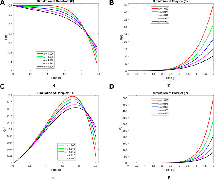
FIGURE 2. 2D-Simulation of the reversible enzymatic reaction model with the CPCF operator. (A) Substrate (S), (B) Enzyme (E), (C) Complex (C), (D) Product (P).

FIGURE 3

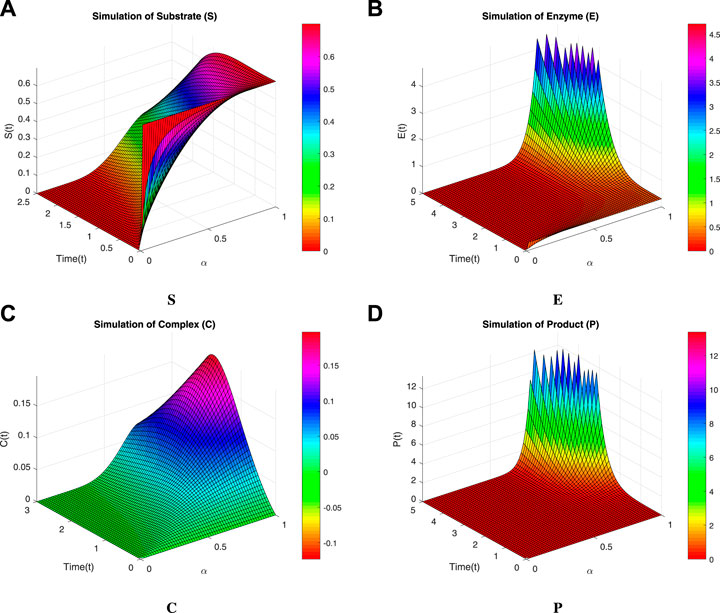
FIGURE 3. 3D-Simulation of the reversible enzymatic reaction model with the CPCF operator. (A) Substrate (S), (B) Enzyme (E), (C) Complex (C), (D) Product (P).

FIGURE 4

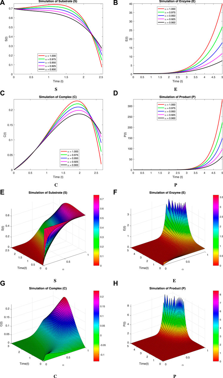
FIGURE 4. Simulation of the reversible enzymatic reaction model with the CPABC operator with 2D-plots from (A) Substrate (S), (B) Enzyme (E), (C) Complex (C), (D) Product (P) and 3D-plots from (E) Substrate (S), (F) Enzyme (E), (G), Complex (C), (H) Product (P).

FIGURE 5

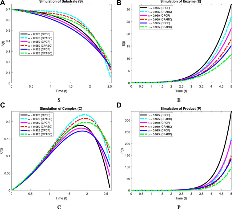
FIGURE 5. Simulation of the reversible enzymatic reaction model with proportional Caputo operators. (A) Substrate (S), (B) Enzyme (E), (C) Complex (C), (D) Product (P).

TABLE 1

TABLE 1. Numerical simulation of the substrate (S).

TABLE 2

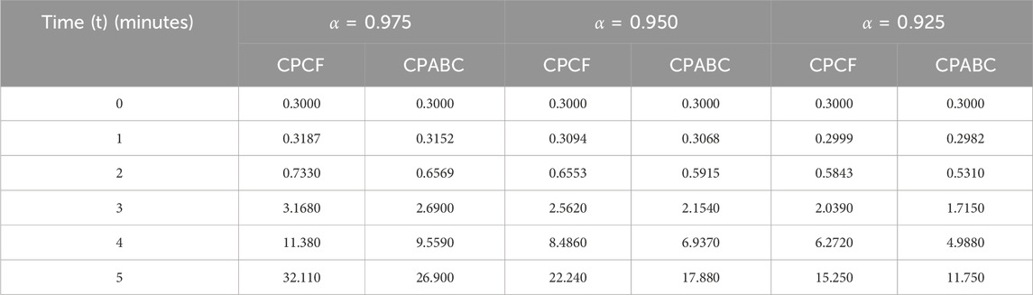
TABLE 2. Numerical simulation of the enzyme (E).

TABLE 3

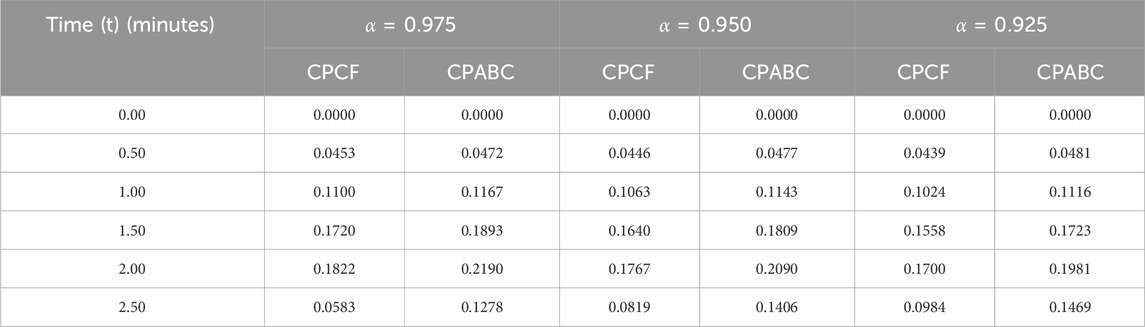
TABLE 3. Numerical simulation of the complex (C).

TABLE 4

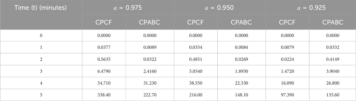
TABLE 4. Numerical simulation of the product (P).

7 Conclusion

The fractional operators CPABC and CPCF, along with the LADM method, were used to analyze the reversible enzymatic reaction model. Existence, singularity, and stability were among the attributes displayed by the solutions. Numerical data were reported, and the simulation results of the hybrid fractional operators were compared. Regarding handling non-linear systems of fractional order, LADM is an excellent analytical method and a potent computational tool for understanding physical problems. The fractional model has the advantage of providing multiple solutions, in contrast to classical models that only have one solution for an integer order. Constant proportional models have more memory compared to integer-order models, which contributes to their use in mathematically simulating the kinetics of enzymes. By adjusting fractional parameters, these operators can enhance the interpretation of enzyme kinetics. Future research can examine chemical reactions in massive reactors and in commercial, animal, and plant environments. It can also solve current models using more general operators.

Data availability statement

The original contributions presented in the study are included in the article/Supplementary Material; further inquiries can be directed to the corresponding author.

Author contributions

PN: conceptualization, methodology, supervision, and writing–original draft. AZ: formal analysis, investigation, and writing–original draft. MF: data curation, formal analysis, software, and writing–original draft. AS: data curation, software, validation, and writing–review and editing. SS: project administration, software, visualization, and writing–review and editing. ZH: funding acquisition, investigation, and writing–review and editing.

Funding

The authors declare that financial support was received for the research, authorship, and/or publication of this article. This work was supported by Research Funding from Youjiang Medical University for Nationalities, China, under grant numbers yy2020bsky050 and yy2023rcky002, the National Natural Science Foundation of China under grant number 62162063, and the Scientific Research and Technology Development Program of Guangxi under grant number 2021AC19308.

Conflict of interest

The authors declare that the research was conducted in the absence of any commercial or financial relationships that could be construed as a potential conflict of interest.

Publisher’s note

All claims expressed in this article are solely those of the authors and do not necessarily represent those of their affiliated organizations, or those of the publisher, the editors, and the reviewers. Any product that may be evaluated in this article, or claim that may be made by its manufacturer, is not guaranteed or endorsed by the publisher.

References

1. Cornish-Bowden A. Fundamentals of enzyme kinetics. John Wiley and Sons (2013).

Google Scholar

2. Rogers A, Gibon Y. Enzyme kinetics: theory and practice. In: Plant metabolic networks. Editor J Schwender. New York, NY (2009). p. 71–103. doi:10.1007/978-0-387-78745-9_4

CrossRef Full Text | Google Scholar

3. Khan M, Ahmad Z, Ali F, Khan N, Khan I, Nisar KS. Dynamics of two-step reversible enzymatic reaction under fractional derivative with Mittag-Leffler Kernel. Plos one (2023) 18(3):e0277806. doi:10.1371/journal.pone.0277806

PubMed Abstract | CrossRef Full Text | Google Scholar

4. Xie XS. Enzyme kinetics, past and present. Science (2013) 342(6165):1457–9. doi:10.1126/science.1248859

PubMed Abstract | CrossRef Full Text | Google Scholar

5. Gao J, Truhlar DG. Quantum mechanical methods for enzyme kinetics. Annu Rev Phys Chem (2002) 53(1):467–505. doi:10.1146/annurev.physchem.53.091301.150114

PubMed Abstract | CrossRef Full Text | Google Scholar

6. Liao W, Liu Y, Wen Z, Frear C, Chen S. Kinetic modeling of enzymatic hydrolysis of cellulose in differently pretreated fibers from dairy manure. Biotechnol Bioeng (2008) 101(3):441–51. doi:10.1002/bit.21921

PubMed Abstract | CrossRef Full Text | Google Scholar

7. Rigouin C, Ladrat CD, Sinquin C, Colliec-Jouault S, Dion M. Assessment of biochemical methods to detect enzymatic depolymerization of polysaccharides. Carbohydr Polym (2009) 76(2):279–84. doi:10.1016/j.carbpol.2008.10.022

CrossRef Full Text | Google Scholar

8. Lorsch JR. Practical steady-state enzyme kinetics. Methods Enzymol (2014) 536:3–15. doi:10.1016/b978-0-12-420070-8.00001-5

PubMed Abstract | CrossRef Full Text | Google Scholar

9. Gan Q, Allen SJ, Taylor G. Kinetic dynamics in heterogeneous enzymatic hydrolysis of cellulose: an overview, an experimental study, and mathematical modeling. Process Biochem (2003) 38(7):1003–18. doi:10.1016/S0032-9592(02)00220-0

CrossRef Full Text | Google Scholar

10. Wu CS, Wu CT, Yang YS, Ko FH. An enzymatic kinetics investigation into the significantly enhanced activity of functionalized gold nanoparticles. Chem Commun (2008)(42) 5327–9. doi:10.1039/b810889g

PubMed Abstract | CrossRef Full Text | Google Scholar

11. Naik PA. Global dynamics of a fractional-order SIR epidemic model with memory. Int J Biomathematics (2020) 13(8):2050071. doi:10.1142/s1793524520500710

CrossRef Full Text | Google Scholar

12. Meena A, Eswari A, Rajendran L. Mathematical modelling of enzyme kinetics reaction mechanisms and analytical solutions of non-linear reaction equations. J Math Chem (2010) 48(2):179–86. doi:10.1007/s10910-009-9659-5

CrossRef Full Text | Google Scholar

13. Ahmad A, Farman M, Naik PA, Saleem MU, Akgul A. Modeling and numerical investigation of fractional-order bovine babesiosis disease. Numer Methods Partial Differential Equations (2021) 37(3):1946–64. doi:10.1002/num.22632

CrossRef Full Text | Google Scholar

14. Naik PA, Eskandari Z, Madzvamuse A, Avazzadeh Z, Zu J. Complex dynamics of a discrete-time seasonally forced SIR epidemic model. Math Methods Appl Sci (2023) 46(6):7045–59. doi:10.1002/mma.8955

CrossRef Full Text | Google Scholar

15. Guariglia E. Harmonic Sierpinski gasket and applications. Entropy (2018) 20(9):714. doi:10.3390/e20090714

PubMed Abstract | CrossRef Full Text | Google Scholar

16. Guariglia E. Primality, fractality, and image analysis. Entropy (2019) 21(3):304. doi:10.3390/e21030304

PubMed Abstract | CrossRef Full Text | Google Scholar

17. Guido RC, Pedroso F, Contreras RC, Rodrigues LC, Guariglia E, Neto JS. Introducing the Discrete Path Transform (DPT) and its applications in signal analysis, artefact removal, and spoken word recognition. Digital Signal Process. (2021) 117:103158. doi:10.1016/j.dsp.2021.103158

CrossRef Full Text | Google Scholar

18. Yang L, Su H, Zhong C, Meng Z, Luo H, Li X, et al. Hyperspectral image classification using wavelet transform-based smooth ordering. Int J Wavelets, Multiresolution Inf Process (2019) 17(06):1950050. doi:10.1142/s0219691319500504

CrossRef Full Text | Google Scholar

19. Zheng X, Tang YY, Zhou J. A framework of adaptive multiscale wavelet decomposition for signals on undirected graphs. IEEE Trans Signal Process (2019) 67(7):1696–711. doi:10.1109/tsp.2019.2896246

CrossRef Full Text | Google Scholar

20. Ragusa MA. On some trends on regularity results in Morrey spaces. in AIP conference proceedings. American Institute of Physics (2012):770–7.

CrossRef Full Text | Google Scholar

21. Khan T, Rihan FA, Ahmad H. Modelling the dynamics of acute and chronic hepatitis B with optimal control. Scientific Rep (2023) 13(1):14980. doi:10.1038/s41598-023-39582-9

CrossRef Full Text | Google Scholar

22. Dehingia K, Das A, Hincal E, Hosseini K, El Din SM. Within-host delay differential model for SARS-CoV-2 kinetics with saturated antiviral responses. Math Biosciences Eng (2023) 20(11):20025–49. doi:10.3934/mbe.2023887

CrossRef Full Text | Google Scholar

23. Partohaghighi M, Mortezaee M, Akgül A, Hassan AM, Sakar N. Numerical analysis of the fractal-fractional diffusion model of ignition in the combustion process. Alexandria Eng J (2024) 86:1–8. doi:10.1016/j.aej.2023.11.038

CrossRef Full Text | Google Scholar

24. Khan I, Nawaz R, Ali AH, Akgül A, Lone SA. Comparative analysis of the fractional order Cahn-Allen equation. Partial Differential Equations Appl Maths (2023) 8:100576. doi:10.1016/j.padiff.2023.100576

CrossRef Full Text | Google Scholar

25. Li C, Dao X, Guo P. Fractional derivatives in complex planes. Nonlinear Anal Theor Methods Appl (2009) 71(5-6):1857–69. doi:10.1016/j.na.2009.01.021

CrossRef Full Text | Google Scholar

26. Guariglia E. Riemann zeta fractional derivative functional equation and link with primes. Adv Difference Equations (2019) 2019(1):261–15. doi:10.1186/s13662-019-2202-5

CrossRef Full Text | Google Scholar

27. Guariglia E, Silvestrov S. Fractional-wavelet analysis of positive definite distributions and wavelets on D’(C) D’(C). In: Engineering mathematics II: algebraic, stochastic and analysis structures for networks, data classification and optimization. Springer International Publishing (2016). p. 337–53.

CrossRef Full Text | Google Scholar

28. Berry MV, Lewis ZV, Nye JF. On the weierstrass-mandelbrot fractal function. Proceedings of the royal society of London. A. Math Phys Sci (1980) 370(1743):459–84. doi:10.1098/rspa.1980.0044

CrossRef Full Text | Google Scholar

29. Farman M, Akgül A, Nisar KS, Ahmad D, Ahmad A, Kamangar S, et al. Epidemiological analysis of fractional order COVID-19 model with Mittag-Leffler kernel. AIMS Maths (2022) 7(1):756–83. doi:10.3934/math.2022046

CrossRef Full Text | Google Scholar

30. Sajjad A, Farman M, Hasan A, Nisar KS. Transmission dynamics of fractional order yellow virus in red chili plants with the Caputo-Fabrizio operator. Mathematics Comput Simulation (2023) 207:347–68. doi:10.1016/j.matcom.2023.01.004

CrossRef Full Text | Google Scholar

31. Sivashankar M, Sabarinathan S, Nisar KS, Ravichandran C, Kumar BS. Some properties and stability of Helmholtz model involved with nonlinear fractional difference equations and its relevance with quadcopter. Chaos, Solitons and Fractals (2023) 168:113161. doi:10.1016/j.chaos.2023.113161

CrossRef Full Text | Google Scholar

32. Al-Basir F, Elaiw AM, Kesh D, Roy PK. Optimal control of a fractional-order enzyme kinetic model. Control and Cybernetics (2015) 44(4):443–61.

Google Scholar

33. Akinyemi ST, Salami SA, Akinyemi IB, Sahabi S. Analytic solution of a time fractional enzyme kinetics model using differential transformation method and pade approximant. Int J Appl Sci Math Theor (2017) 3(3):25–32.

Google Scholar

34. Dubey VP, Kumar R, Kumar D. Approximate analytical solution of fractional order biochemical reaction model and its stability analysis. Int J Biomathematics (2019) 12(05):1950059. doi:10.1142/s1793524519500591

CrossRef Full Text | Google Scholar

35. Akgül A, Khoshnaw SA. Application of fractional derivative on non-linear biochemical reaction models. Int J Intell Networks (2020) 1:52–8. doi:10.1016/j.ijin.2020.05.001

CrossRef Full Text | Google Scholar

36. Alqhtani M, Saad KM. Fractal-fractional michaelis-menten enzymatic reaction model via different kernels. Fractal and Fractional (2021) 6(1):13. doi:10.3390/fractalfract6010013

CrossRef Full Text | Google Scholar

37. Akgül A. Some fractional derivatives with different kernels. Int J Appl Comput Maths (2022) 8(4):183. doi:10.1007/s40819-022-01389-z

CrossRef Full Text | Google Scholar

38. Baleanu D, Fernandez A, Akgül A. On a fractional operator combining proportional and classical differ integrals. Mathematics (2020) 8(3):360. doi:10.3390/math8030360

CrossRef Full Text | Google Scholar

39. Farman M, Alfiniyah C, Shehzad A. Modelling and analysis tuberculosis (TB) model with hybrid fractional operator. Alexandria Eng J (2023) 72:463–78. doi:10.1016/j.aej.2023.04.017

CrossRef Full Text | Google Scholar

40. ul Haq I, Ali N, Ahmad H, Sabra R, Albalwi MD, Ahmad I. Mathematical analysis of a coronavirus model with Caputo, Caputo-Fabrizio-Caputo fractional and Atangana-Baleanu-Caputo differential operators. Int J Biomathematics (2023):2350085. doi:10.1142/s1793524523500857

CrossRef Full Text | Google Scholar

41. Rezapour S, Asamoah JKK, Etemad S, Akgül A, Avci I, El Din SM. On the fractal-fractional Mittag-Leffler model of a COVID-19 and Zika Co-infection. Results Phys (2023) 55:107118. doi:10.1016/j.rinp.2023.107118

CrossRef Full Text | Google Scholar

42. Sweilam N, Al-Mekhlafi SM, Salama RG, Assiri TA. Numerical simulation for a hybrid variable-order multi-vaccination COVID-19 mathematical model. Symmetry (2023) 15(4):869. doi:10.3390/sym15040869

CrossRef Full Text | Google Scholar

43. Nisar KS, Farman M, Hincal E, Shehzad A. Modelling and analysis of bad impact of smoking in society with Constant Proportional-Caputo Fabrizio operator. Chaos, Solitons and Fractals (2023) 172:113549. doi:10.1016/j.chaos.2023.113549

CrossRef Full Text | Google Scholar

44. Attia N, Akgül A, Seba D, Nour A, la Sen MD, Bayram M. An efficient approach for solving differential equations in the frame of a new fractional derivative operator. Symmetry (2023) 15(1):144. doi:10.3390/sym15010144

CrossRef Full Text | Google Scholar

45. Nisar KS, Farman M, Abdel-Aty M, Cao J. A review on epidemic models in sight of fractional calculus. Alexandria Eng J (2023) 75:81–113. doi:10.1016/j.aej.2023.05.071

CrossRef Full Text | Google Scholar

46. Naik PA, Eskandari Z, Shahraki HE. Flip and generalized flip bifurcations of a two-dimensional discrete-time chemical model. Math Model Numer Simulation Appl (2021) 1(2):95–101. doi:10.53391/mmnsa.2021.01.009

CrossRef Full Text | Google Scholar

47. Li C, Qian D, Chen Y. On Riemann-Liouville and caputo derivatives. Discrete Dyn Nat Soc (2011) 2011:1–15. doi:10.1155/2011/562494

CrossRef Full Text | Google Scholar

48. Anderson DR, Ulness DJ. Newly defined conformable derivatives. Adv Dynamical Syst Appl (2015) 10(2):109–37.

Google Scholar

49. Caputo M, Fabrizio M. A new definition of fractional derivative without singular kernel. Prog Fractional Differ Appl (2015) 1(2):73–85.

Google Scholar

50. Atangana A, Baleanu D. New fractional derivatives with nonlocal and non-singular kernel: theory and application to heat transfer model (2016). arXiv preprint arXiv:1602.03408.

Google Scholar