 Juliana Bibiano
 Jonas Kleineisel1
 Anne Slawig
94% of researchers rate our articles as excellent or good
Learn more about the work of our research integrity team to safeguard the quality of each article we publish.
Find out more
ORIGINAL RESEARCH article
Front. Phys., 18 January 2024
Sec. Medical Physics and Imaging
Volume 11 - 2023 | https://doi.org/10.3389/fphy.2023.1299522
This article is part of the Research TopicEditor's Challenge in Medical Physics and Imaging: Quantitative Medical ImagingView all 11 articles
Introduction: Quantification of longitudinal relaxation time T1 gained interest as an important MR-inducible tissue property for tissue characterization. Standard inversion recovery (IR) measurements for T1 determination take a prohibitively long time, and signal models assume a perfect inversion. Acceleration is possible by using the Look–Locker (LL) technique or other accelerated, model-based algorithms. However, the calculation of real T1 values from LL acquisitions necessitates the knowledge of equilibrium magnetization M0. Thus, usually, a waiting time to allow for free relaxation between global inversion pulses must be implemented. This study aims to introduce a novel model-based fitting approach for T1 mapping without the need for such waiting times.
Methods: Single-inversion spiral LL spoiled gradient echo acquisitions were performed in a phantom and eight healthy volunteers using a 1.5T magnetic resonance imaging (MRI) scanner. The measurements comprised two parts, one without magnetization preparation and a second featuring a global inversion pulse preparation before each of the 35 slices. Acquisition was performed without any waiting time in between slices, i.e., before the inversion pulses. T1 maps were calculated based on an iterative model-based reconstruction algorithm which combines the information from these two measurements, with and without inversion.
Results: Accurate T1 maps were obtained in phantom and volunteer measurements. ROI-based mean T1 values differ by an average of 1.5% in the phantom and 5% in vivo between reference measurements and the proposed method. The combined fit benefits from both the information obtained in the inversion prepared and the unprepared measurements. The former provides a large dynamic range for accurate model-based fitting of the relaxation process, while the latter provides equilibrium magnetization M0, necessary to obtain accurate T1 values from a LL-like acquisition.
Conclusion: The proposed model of a combined fit of an inversion-prepared and an unprepared measurement allows for robust fast T1 mapping, even in cases of imperfect inversion due to skipped waiting times for magnetization recovery. Thus, it can render long waiting times in between inversion pulses redundant.
Quantitative magnetic resonance imaging (MRI) allows obtaining maps of specific physical parameters in MRI. When compared to qualitative MRI (or weighted imaging), it additionally allows
- comparison of different tissues within the same individual from different locations or points in time;
- comparison between images from different individuals; and
- achievement of disease-specificity, with studies correlating abnormalities in the absolute values of certain MR-inducible tissue properties and health conditions [1–4].
The quantification of longitudinal relaxation time T1 gained interest for tissue characterization, and T1 mapping is already used in cardiac [1, 2, 5] and brain MRI [3, 4, 6]. Conventional techniques for T1 determination are based on tracking magnetization after a suitable magnetization preparation, e.g., inversion recovery (IR) measurements. Following an inversion pulse, an image is acquired for a fixed delay after the inversion pulse. Typically, the k-space is filled in a segmented fashion. Consequently, for each repetition, magnetization must be restored to the original state, requiring a waiting interval to ensure full recovery of the signal before every new magnetization preparation. Repetitions of these measurements, to acquire images at different delays after the inversion pulse, are necessary to trace the relaxation of magnetization. Thus, standard IR measurements have a prohibitively long duration and are hardly feasible for clinical application [6–8]. The Look–Locker (LL) technique [9] came as a milestone for accelerated T1 quantification. Typically, an IR magnetization preparation pulse is applied, followed by a series of low-angle radiofrequency (RF) pulses used for spoiled gradient echo imaging. Data acquired after one inversion is sorted into different k-spaces, corresponding to the different delays after the inversion. Thus, the number of necessary repetitions can be reduced compared to conventional IR T1 mapping. However, the problem of the long waiting periods, on the order of 5*T1max, still exists for the LL technique [2, 10]. Although LL techniques are much faster than conventional IR T1 mapping, the RF pulses used for data acquisition affect the T1 recovery. Thus, the longitudinal relaxation process is not the same as for an undisturbed IR experiment, resulting in an apparent T1 (termed T1*). The longitudinal relaxation time T1 can be calculated from the apparent relaxation time T1* using the acquisition parameters repetition time and the local flip angle [11, 12]. Alternatively, T1 can be calculated from the measured quantities, T1*, equilibrium magnetization M0, and steady-state magnetization Mss [10, 12]:
Based on a novel model-based fitting approach, this study aims to introduce a technique for T1 mapping without the necessity of waiting times for free relaxation in between inversion pulses.
Measurements were performed on eight healthy volunteers. The study was approved by the local ethics committee, and informed consent was obtained from all volunteers before scanning. Experiments were performed on a 1.5T MRI scanner (Siemens MAGNETOM Avanto Fit) using a 20-channel head coil array. Table 1 gives an overview of all measurements performed. In general, reference measurements were performed using a turbo spin echo (TSE) sequence (Table 1, Nb 1 and 3), while acquisitions for the proposed method are based on a LL [9], spoiled gradient echo acquisition with a spiral trajectory (Table 1, Nb. 2A, 2B, 4A, 4B, 5A, and 5B).
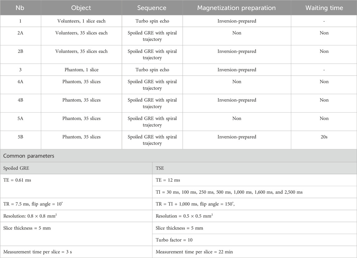
TABLE 1. Overview of measurements and their measurement parameters.
For comparison, in each volunteer and the phantom examination, one slice was acquired using a TSE sequence using the following imaging parameters: flip angle = 150°, resolution = 0.5 × 0.5 mm2, slice thickness = 5 mm, turbo factor = 10, measurement time = 22 min, and TE = 12 ms. Inversion times were as follows: TI = 30 ms, 100 ms, 250 ms, 500 ms, 1,000 ms, 1,600 ms, and 2,500 ms, and TR was TI + 1,000 ms and ranged between 1,030 and 3,500 ms. In the phantom, measurements at TI = 6,000 ms and 10,000 ms were added.
For all other acquisitions in each slice, 400 spoiled gradient echoes (GREs) using a variable-density spiral read-out trajectory were acquired. Consecutive spiral arms were spaced apart by a double golden angle. The trajectory was designed using the variable-density spiral design function tool [16, 17] by Brian Hargreaves and adjusted to observe a maximum gradient amplitude of 40 mT/m and a maximum gradient slew rate of 170 mT/m/s. The readout length of one spiral arm was 6.28 ms and extended in k-space to a maximum value of 0.625 1/mm in order to achieve a spatial resolution of 0.8 × 0.8 mm2. By design, a total of 70 equally spaced spiral arms could fully cover the k-space for a FOV of 300 mm. However, in this study, a continuous rotation of a double golden angle was chosen between consecutive spiral arms. Other imaging parameters include TE = 0.61 ms, TR = 7.5 ms, flip angle = 10°, slice thickness = 5 mm, and measurement time = 3s for each slice. Each acquisition in a healthy volunteer comprised 35 slices in interleaved order and covered the whole brain.
These measurements comprised two LL-like acquisition parts: during the first part (Nb. 2A), no preparation and only slice-selective excitations were used. In the second part (Nb. 2B), a global adiabatic inversion pulse was applied before the acquisition of each slice (pulse length: 10.2 ms). No waiting time was heeded in between slices, and thus, starting magnetization was affected by the previous global inversion pulses. Both parts acquire the course of the receiver coil weighted magnetization from a starting point (M0 or –αM0) to the steady-state magnetization Mss.
The same protocol was used for phantom measurements (Nb. 4A and 4B) on an Essential System Phantom Model 106 by CaliberMRI (Handbook T1 values are given in Table 2). Here, an additional measurement with a waiting time of 20 s in between slices, and thus in between successive inversion pulses, was performed (Nb. 5A, 5B). The value of more than 10*maximum T1 in the phantom was chosen to ensure full relaxation of all phantom compartments and no signal contamination by former inversion pulses. Additionally, reference T1 values for the different vials within the phantom are provided by the vendor in the phantom manual.
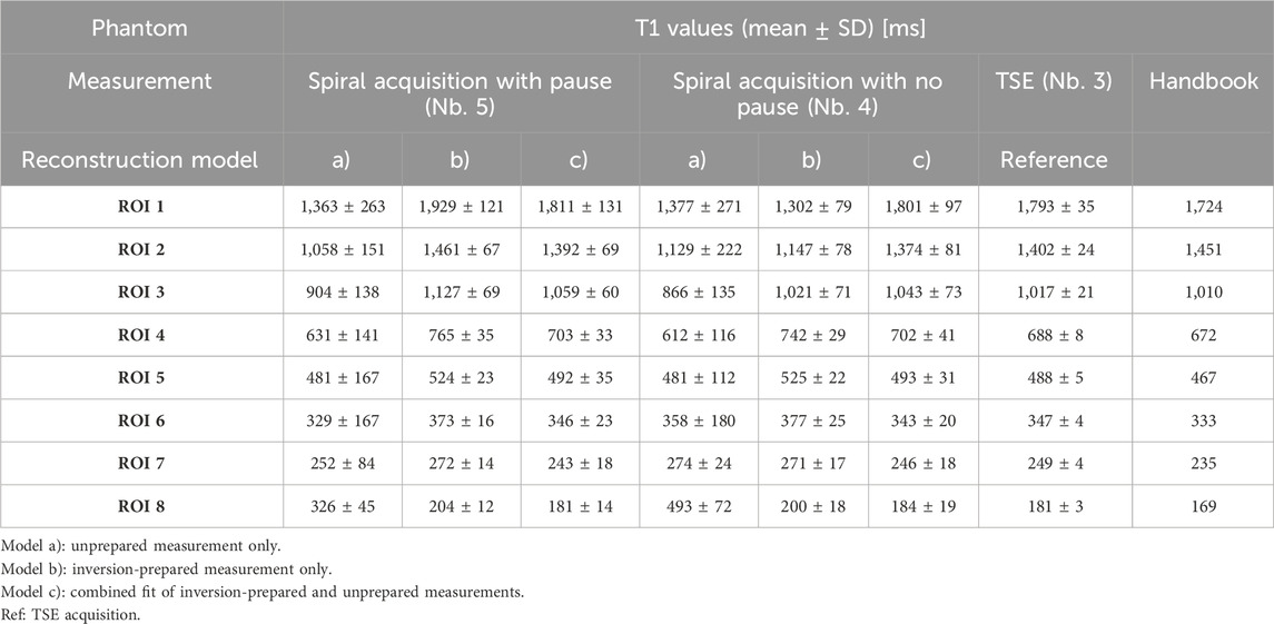
TABLE 2. T1 values as determined in the phantom measurements.
A depiction of the spoiled gradient echo pulse sequence and the spiral k-space trajectory is given in Figure 1.
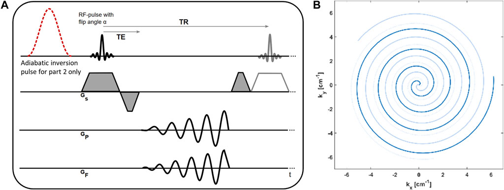
FIGURE 1. (A) Sequence diagram of the spoiled gradient echo acquisition with spiral trajectory. In part one of the measurement, no magnetization preparation is performed. In part two of the measurement, the nonselective adiabatic inversion pulse is played out before the acquisition of each slice. (B) Depiction of the spiral trajectory. Shown are the first three arms, and consecutive arms are continuously rotated by a double golden angle.
For all measurements, raw data was extracted from the scanner, and image reconstruction was performed offline in MATLAB. Reference TSE measurements (Table 1, Nb. 1 and 3) were reconstructed by 2D Fourier transform. Data reconstruction of spiral GRE acquisitions was performed by a modified model-based acceleration of LL T1 mapping (MAP) algorithm [10, 15]. First, the corrected spiral k-space trajectory was calculated based on the gradient system transfer function [18, 19]. Then, initial images were reconstructed by gridding the data of each spiral arm into separate k-spaces. All reconstructions were performed on a matrix of size 512 × 512 and with a field of view of 40.96 cm. After 2D Fourier transform, this results in a stack of highly undersampled images, which track the time course of T1* relaxation. As one spiral arm is gridded to each k-space, the temporal resolution equals TR. This was conducted separately for both parts of the spiral measurements, with and without the inversion pulse.
This initial step was followed by the iterative reconstruction algorithm consisting of alternating steps of pixel-wise model-based fitting and restoring data consistency. Data from the two parts of the measurement (Nb. 2A and B, 4A and B, and 5A and B) was either reconstructed together using a combined model (model (c)) or, for comparison, separately only for the unprepared part (model (a) for part A) or the inversion-prepared part (model (b) for part B).
This pixel-wise fitting of the reconstruction used the following fitting models:
(a) Unprepared:
The transient phase of unprepared magnetization in spoiled gradient echo acquisition only (Nb. 2A, 4A, and 5A) with three free parameters (M0non, Mss, and T1*):
(b) Inversion-prepared:
Inversion recovery Look–Locker (IR-LL) acquisition only (Nb. 2B, 4B, and 5B) with three free parameters (M0IR, Mss, and T1*):
(c) Combined:
A combination of unprepared GRE magnetization and magnetization of IR-LL acquisitions (Nb. 2A and B, 4A and B, and 5A and B) with four free parameters (M0IR, M0non, Mss, and T1*):
where Mss is steady-state magnetization, T1* is the LL relaxation time [9], M0non is equilibrium magnetization, and M0IR is magnetization directly after the inversion pulse. An illustration of the different models for data on representative voxels is given in Figure 2. Afterward, fitted images were transformed back to the k-space, and data consistency was enforced by reintroducing measured data points into these modeled k-spaces. As in the original MAP algorithm, we iteratively performed steps consisting of model-based fitting and data consistency until convergence to a solution was reached [15].
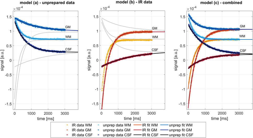
FIGURE 2. Comparison of the different fit models for three exemplary pixels in the white matter (WM), gray matter (GM), and cerebrospinal fluid (CSF), as performed in the last iteration. Data and fits of inversion prepared measurements are shown in shades of blue, from unprepared measurements in shades of red. Left: Fit of three parameters (Mss, M0non, and T1*) on data on the unprepared measurement (part A of spiral LL acquisitions), as described by model (a). Center: Fit of three parameters (Mss, M0IR, and T1*) on data on the inversion prepared measurement (part B of spiral LL acquisitions), as described by model (b). Right: combined fit of four parameters (Mss, M0IR, M0non, and T1*) on data on the unprepared and inversion-prepared measurement simultaneously, as described by model (c). Major difference lies in the constraint introduced by model (c), forcing Mss and T1* to be similar in both relaxation processes.
However, as this procedure converges rather slowly, we used a modified algorithm. The original MAP reconstruction algorithm can be seen as alternating projections onto two different subspaces: the data-consistent solutions and the subspace of exponential signal evolutions in all pixels. A combination of two MAP projections, either from the data-consistent solution subspace back onto the data-consistent solution subspace or from the exponential model subspace back to the model subspace, can be seen as steps into the right direction with a non-optimized step size. In other words, from two solutions in each of these subspaces, a one-dimensional (1D) consistency subspace and a 1D model subspace are defined. In the modified MAP algorithm, we calculate the point in the 1D data-consistent subspace, which is closest to the 1D model subspace, and use it as the starting points for two further MAP iterations. These MAP steps were used again to determine new 1D subspaces and a new step size estimate. If the reconstruction problem would be linear and the measured data without noise, the exact solution would be found after a single step size adjustment. Numerical experiments suggest that, for our data, this approach reduces the number of steps before convergence by a factor of approximately 50 compared to the original MAP approach while arriving at a similar solution. For the reconstructions presented below, we performed six MAP steps and two step size adjustments (after MAP steps 2 and 4) in total.
From the results of the last iteration in the model-based subspace, absolute T1 values were calculated from the apparent relaxation time T1* in LL acquisitions as [10]:
Reference TSE data were reconstructed by 2D FFT, and an adaptive coil combination was performed [20]. The average phase of the last three measurements in each pixel was subtracted from all measurements, and subsequently, the real part of the data was fitted pixel-wise using the following equation (adapted from [21]):
with
where TR is the repetition time and TI is time after inversion. Parameters b and c account for a potential non-ideal inversion and a constant effect of the acquired multi-echo train, respectively.
In each multi-slice measurement, the central slice was identified, which also corresponds to the slice chosen in single-slice reference measurements. ROIs were then manually placed in corresponding areas in all measurements. In the phantom, a total of eight circular ROIs were added to comprise each of the separate vials inside the phantom. These ROIs were labeled ROI 1 to ROI 8 in the order of decreasing T1 values. In each volunteer, three different polygonal ROIs were drawn within that selected slice. The first ROI is placed in the frontal white matter area, the second ROI in the gray matter in the sulci in the right posterior brain, and the third ROI inside the frontal part of one ventricle. For each ROI in the phantom, the mean T1 values and the standard deviation (SD) within the ROI are evaluated. In each volunteer mean T1 values and SD within the ROI are evaluated, as well as mean T1 values and SD in each tissue over the whole group of volunteers.
Additionally, equivalence testing was performed to assess whether the phantom measurements with and without the waiting time were statistically equivalent. Specifically, the two one-sided t-test (TOST) procedure was conducted to test whether the difference in means between two groups falls within a predefined equivalence margin [22]. The equivalence bounds were set to be 3% of the mean T1 value in the reference measurement (i.e., 59 ms in ROI 1, 44 ms in ROI 2, 32 ms in ROI 3, 21 ms in ROI 4, 15 ms in ROI 5, 10 ms in ROI 6, 7 ms in ROI 7, and 5 ms in ROI 8). Practically, the equivalence of the means was assessed by examining whether the 90% confidence interval fell entirely within the predetermined equivalence bounds. Values within each ROI were considered as paired as the same ROIs were applied and pixel values were listed in the same order. The significance level was set at α = 0.05.
Exemplarily, Figure 2 shows the signal evolution in three pixels located in the white matter area in the center of the brain, gray matter area, and cerebrospinal fluid (CSF) in the ventricle. Shown are the data points after data consistency was restored and the corresponding exponential curves fitted in the last iteration of each of the separate reconstruction processes (model (a), model (b), and model (c)). Note that the combined fitting, as proposed in model (c), forces Mss and T1* to be similar for both relaxation processes as data from identical tissue should feature identical tissue properties. Separate fitting of either inversion-prepared data (model (a)) or unprepared data (model (b)) imposes no such constraint, resulting in differing values.
Figure 3 shows parameter maps, as determined by the three different models after eight iteration steps. The combined model (c) yields two values for equilibrium magnetization M0IR and M0non, from the inverted and unprepared relaxation processes respectively, while steady-state magnetization Mss and T1* times are preordained to be identical. Steady-state magnetization Mss (Figure 3 Mss) is comparable in all models. Maps of the equilibrium magnetization M0IR/non are shown in Figure 3 M0. Using model (b) for fitting of inversion-prepared data only (part B of LL measurements) enables robust fitting. Challenges to this model (b) arise in cases of imperfect inversion or altered magnetization due to the lack of waiting time between consecutive global inversions. The latter is especially apparent in areas with long relaxation times like in CSF, where the calculated values of M0IR are low. Low M0IR values are also determined by the combined model, but in contrast, it can robustly determine M0non, and the resulting maps show a similar distribution as in the reference measurement.
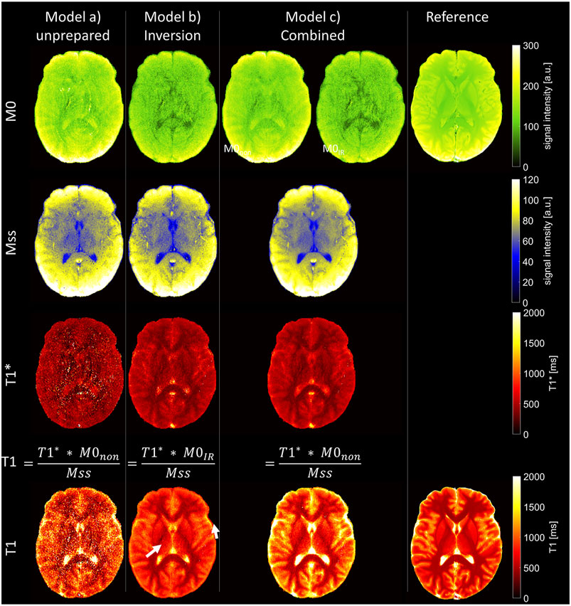
FIGURE 3. Parameter maps as determined by the three different fit models and from the reference measurement. Top: equilibrium magnetization (M0). In the combined fit, two independent parameters (M0IR and M0non) are considered to allow for imperfect inversion. Center: steady-state magnetization (Mss) and apparent longitudinal relaxation times (T1*). Bottom: longitudinal relaxation times (T1), as calculated from fit parameters of unprepared acquisition only [model (a)], inversion-prepared data only [model (b)], and the combined fit of both parts of the measurements [model (c)]. Arrows point to areas of T1 underestimation.
T1* maps (Figure 3 T1*) are noisy when determined by model (a) from unprepared data only. The maps determined by model (b) or (c) show reduced tissue contrast as usual for T1* in LL acquisitions [23–26].
T1 maps, as calculated from these fitting parameters, are shown in Figure 3 T1. The calculation of T1 depends on the accurate determination of T1*, Mss, and M0. Although the first is challenging in model (a), the last poses a problem in model (b). In model (c), equilibrium magnetization is determined by M0non, allowing robust T1 calculation, as reflected in the detailed T1 map (Figure 3 T1).
The results of all 35 slices in the exemplary volunteer are shown in Figure 4. Reasonable T1 maps were acquired at all positions in the head and were independent of the chronological position of the slice in the measurement setup and, therefore, independent of its history of inversion pulses.
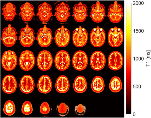
FIGURE 4. T1 maps as determined by the proposed combined fit model (c) in all slices of the whole head of one exemplary volunteer.
The efficiency of the inversion preparation is shown in Figure 5. Clearly, the relaxation process does not start at 100% inversion of equilibrium magnetization M0 in tissues with long relaxation time but in many other areas.
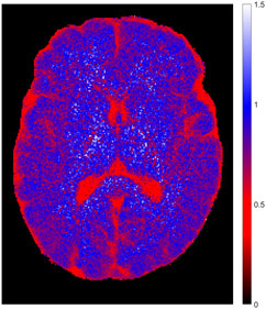
FIGURE 5. Inversion efficiency for one exemplary volunteer, as determined by the ratio of the two parameters M0IR and M0non in the combined fit model (c). Full inversion was not achieved in tissues with long relaxation time but worked fine in other areas.
Figure 6 shows the T1 maps, as determined in the phantom measurements with and without a deliberate waiting time in between slices and, therefore, before all global inversion pulses. Corresponding T1 values from the ROI-based analysis are collected in Table 2. The parameter maps (Mss, M0, T1*, and T1), as determined by the three different fit models after the eighth iteration step are presented in Supplementary Figure S1.
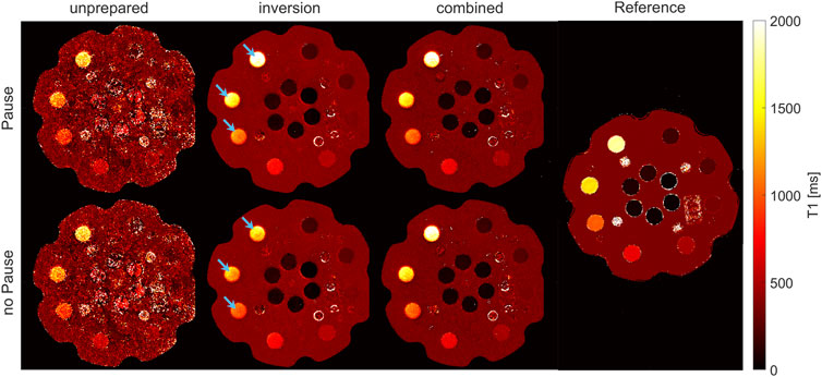
FIGURE 6. T1 maps of phantom measurement, with and without a waiting time to allow for free relaxation of magnetization. Maps calculated from the unprepared measurement by model (a) are noisy, while robust fitting was possible in the inversion-prepared case (model (b)) and with the proposed combined model (c). The major difference between measurements with and without waiting time emerges when regarding vials with long T1 values (indicated by arrows) and the inversion measurement only (model (b) for measurement part B). Measurements without waiting time result in a variable underestimation of absolute T1 values, which can be mitigated by either introducing the waiting time of 20 s or by using the combined model (c).
As in the volunteer, maps calculated from the unprepared measurement (Nb. 2A) with model (a) are noisy, while robust fitting was possible in the inversion-prepared case (Nb. 2B) with model (b) and with the proposed combined reconstruction (Nb. 2A and B) by model (c).
The statistical equivalence test for the combined reconstruction model (model (c)) revealed that the mean difference between T1 values from measurements with and without pause was below the equivalence bounds in all ROIs. Tests on the T1 values gained by model (b) from IR measurements showed that the mean difference was below the equivalent bounds in ROIs 5–8. T1 values in the ROIs 1–4, featuring the longest T1 values, cannot be considered equivalent within the given bounds. Tests for reconstruction model (a), unprepared measurement, revealed that the mean difference between T1 values from measurements with and without pause was outside the equivalence bounds in all ROIs, except for ROI 5.
Deviations of ROI-based mean T1 values between the combined fit model (c) and the TSE reference measurement were 0.4%, 2.0%, 2.5%, 2.0%, 1.0%, 1.2%, 1.2% and 1.6%, respectively, for the eight ROIs in the decreasing T1 order. Deviations to phantom manual values were 4.3%, 5.6%, 3.2%, 4.3%, 5.3%, 2.9%, 4.5%, 8.2%, respectively, for ROIs 1–8 (see also Supplementary Table S1).
T1 maps were calculated for all slices in all eight healthy volunteers and by all three reconstruction models. The T1 maps acquired from the TSE reference measurement and T1 maps calculated from the combined model (c) in a corresponding slice are shown in Supplementary Figure S2. Mean T1 and SD, as calculated by model (a), were 1,567 ± 139 ms in CSF, 967 ± 37 ms in the gray matter, and 529 ± 43 ms in the white matter. Mean T1 and SD, as calculated by model (b), were 2,278 ± 240 ms in CSF, 1,022 ± 44 ms in the gray matter, and 559 ± 84 ms in the white matter. For the combined model (c), mean T1 values and SD of 2,911 ± 240 ms in CSF, 1,198 ± 58 ms in the gray matter, and 557 ± 40 ms in the white matter were found. Separate results for each volunteer and area are collected in Table 3, relative deviations are collected in Supplementary Table S2. In general, model (a) underestimates T1 values and has high SD within the ROIs in each volunteer. Model (b) has lower SD within ROIs and shows underestimation of T1 values, especially in tissue with slow relaxation. The results from model (c) agree within the error bounds with the T1 times as determined by the reference measurement and are in good accordance with the literature values [27–29]. In addition, they feature low SD within each of the evaluated areas, indicating robust fitting.
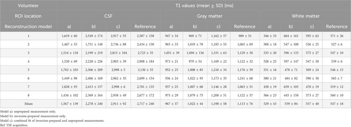
TABLE 3. T1 values determined from ROIs placed in CSF, gray matter, and white matter for the three different fitting models.
The proposed method aims to accomplish fast T1 mapping without the need for waiting times in between inversion pulses. Therefore, the combination of information from two parts of a measurement, with and without inversion, is proposed. To obtain T1 values from a LL acquisition, information on the apparent relaxation time T1* and on equilibrium magnetization M0 and steady-state magnetization Mss is necessary [9, 12]. Inversion-prepared measurements provide a large dynamic range for accurate model-based fitting of the relaxation process (and thus T1*), but without considering the necessary time for magnetization recovery, they cannot provide M0. In contrast, unprepared measurements can provide the equilibrium magnetization M0, but determination of T1* is challenging, due to the low dynamic range of the relaxation process. Information on M0 could, otherwise, be procured by considering long waiting times in between inversion pulses to allow full relaxation before each such pulse. The main advantage of the proposed approach is the omission of such waiting times, which significantly decreases acquisition time.
The design of the spiral trajectory was driven by two limitations. First, the desired resolution and second a limited readout length, in order to prevent strong effects of T2* relaxation along the readout. Furthermore, a variable density factor of two was chosen to optimize the acquisition of the k-space where most of the energy in an image is concentrated near the origin of the k-space [17]. Consecutive spiral arms were rotated in the spiral plane by a double golden angle. One advantage of golden angle sampling is the uniform coverage of the k-space along time. For optimized fitting of the exponential T1 relaxation, ideally, three full k-spaces are available at set points in time. For a fixed T1 value, the ideal position of these in time is known. For unknown multiple T1 values, golden angle sampling provides a good compromise. For center-out trajectory designs, the double golden angle (137.51° ≈ 360°–2*111.25°) features the same properties as the standard golden angle (111.25°) for full spoke acquisitions [30].
Reference multi-inversion TSE measurements were performed in one slice in each volunteer and in the phantom. The settings were adjusted to minimize SAR in all acquisitions and to keep overall scan time within reasonable limits. A variable TR of TI+1,000 ms was chosen for each acquisition in order to realize equal relaxation time in between the last excitation for acquisition and the subsequent inversion pulse. A comprehensive overview of IR signal modeling can be found in MRI handbooks and online (e.g., [21, 31, 32]), including the signal dependencies on TR. In contrast, other measurement setups use constant long TR values (e.g., 5*T1) and include a long TR assumption in the fitting process.
In this study, T1 was determined by multi-inversion TSE measurements, as well as by inversion-prepared and unprepared spiral LL acquisitions in combination with three different fit models. Additionally, handbook values for the phantom are given.
Values given in the phantom handbook are generally lower than measured values (with the exception of ROI 2) independent of the acquisition type and fitting model. For our proposed fitting model (c), deviations are between 2.9% and 8.2%. Differences between the reference measurement and handbook values are in a similar range, between 0.7% and 7.1%. The main reason might be a difference in temperature as handbook values are stated at 20°C, whereas both reference and LL measurements were performed at 22°C–23°C. The temperature dependence of T1 is known to be between 1% and 3% per degree temperature change [33, 34]. Additionally, the reference measurement was performed as a TSE sequence, where the prolonged echo trains average signal around the set TI.
Reconstruction of LL acquisitions by model (a) has low mean T1 values and maps are very noisy, which is also reflected in the high SD within each ROI in the phantom and in all volunteers. Model (b) has lower SD within ROIs but also shows an underestimation of T1 values in comparison to reference measurements or other fitting models, especially in areas with slow relaxation (e.g., ROIs 1 and 2 in phantom or CSF and gray matter in vivo). Due to that, both are not considered a recommended technique.
T1 values, as determined by the proposed combined fit model (c), are in good agreement with reference values obtained by multiple inversion TSE measurements for phantom and in vivo cases. In in vivo measurements, T1 values deviate by 1.8% in the white matter, 7.1% in the gray matter, and 6.6% in CSF, and are in a range of literature values given for the evaluated tissues [27–29]. In the phantom, a T1 range of 150–2,000 ms is covered. Within these ROIs, T1 values deviate by no more than 2.5% from the reference measurement.
For very slow relaxing components (like CSF), inaccuracies can occur due to the short overall LL acquisition time per slice. Although main features of the relaxation process are covered within the 3 s acquisition, the magnetization level of very slow components has not necessarily reached the steady-state magnetization yet.
The main advantage of model-based reconstructions lies in the usage of prior knowledge. The MAP approach applied in this study combines prior knowledge about the relaxation behavior with the contrast information acquired using a spiral sampling scheme [10, 15]. The iterative reconstruction algorithm introduces more and more information about the relaxation process into the initial k-spaces, which originally contain only one spiral arm each. Although, for example, fingerprinting assumes that incoherent artifacts do not influence the fitting, MAP uses the information from other time points to consistently fill each k-space. Thus, over the iterations, the k-space of each point in time is filled and undersampling artifacts are eliminated. As a result, one complete image is generated for every time point TI of the relaxation process. Specifically, for the study presented here, a total of 400 full images spaced apart by TR were obtained.
The relaxation process from equilibrium magnetization (or inversion) into steady-state magnetization depends on T1* and can be fitted by corresponding exponential equations of T1* in inversion-prepared and unprepared measurements. The main advantage of the former is the large dynamic range of signal evolution, which benefits robust fitting, especially in accelerated methods. Unfortunately, to determine equilibrium magnetization M0, it also demands perfect inversion and, thus, a waiting time to allow free relaxation in between pulses. By combining the inversion acquisition with an unprepared measurement, M0 can be adequately recovered in a combined fit, as given by model (c). Thus, no waiting time is necessary. As an additional benefit, the combined fit model allows an investigation of the performance of the inversion pulse by comparing M0non and M0IR.
The main advantage of such a model-based approach is the efficient use of information gathered in the shortest measurement times. Reconstructions can be performed on a fine temporal grid as no binning of phase-encoding steps is used, but each acquired spiral arm provides information on one time point along the relaxation curves. In combination with pixel-wise fitting, no spatial or temporal filtering is applied.
The presented study used a global inversion pulse to provide maximum insensitivity to B1 inhomogeneity [35]. The inversion was then followed by the acquisition of a single slice. Consequently, all slices are affected each time an inversion is played out. In other words, all slices, but the first, have a history of multiple inversions. If no waiting time for free relaxation in between the inversion pulses is heeded, the inversion acts on an arbitrary magnetization vector and not on the equilibrium magnetization M0. Thus, the start point of the relaxation process shifts from –M0, as in a perfect inversion, to a different value, and M0 can no longer be determined. Loss of the M0 information subsequently prevents the necessary T1* correction for LL acquisitions [9, 10, 12].
An additional advantage of a global inversion is that it allows generalization of the method, for example, for segmented 3D [36–38] acquisitions or simultaneous multi-slice measurements [39].
T1 mapping is often included in multiparametric acquisition frameworks [40], like fingerprinting [41–44], the MR multitasking framework [45, 46], or SyMRI [47, 48], which can achieve clinically reasonable scan times below 10 min. Although the additional information gained might be a benefit, the faster acquisition in our proposed method is favorable for dedicated T1 mapping applications.
Another common technique to determine T1 is the variable flip angle method [49]. Several approaches were presented, which can acquire whole-head T1 maps under 10 min [3, 6, 50]. Although they are very fast, they require exact knowledge of the flip angle. Additionally, problems with the B1 inhomogeneity and slice profile may arise, especially for thin slices and fast pulses [51]. T1 values determined by the variable flip angle method are also dependent on the RF spoiling procedure [52].
In techniques based on IR-LL methods, T1 can be calculated from T1* either by using the acquisition parameters repetition time TR and the local flip angle or from the measured quantities, T1*, M0, and Mss [9, 12]. By choosing optimal settings for a given experiment and incorporating flip angle information, a bias from imperfect inversion can be minimized. Shin et al. [11] performed whole brain T1 mapping in approximately 4 min with a resolution of 1 × 1 × 4 mm3. Within an optimized setup, an average error of T1 of 1.2% was achieved, without requiring a specific waiting time in between inversion pulses. In comparison to our approach, this study achieved comparable measurement times, albeit slightly lower in-plane resolution and volume coverage.
Other techniques based on IR-LL methods mostly rely on segmented acquisitions with multiple inversions, especially for 3D acquisitions, which require a high number of readout lines. For example, Henderson et al. [36] performed whole-head T1 mapping with a resolution of 1.4 × 1.4 × 6 mm3 in 8 min. The volume was divided into 128 segments, each starting with an inversion pulse and a delay time of 2 s in between. Similar measurement times were achieved by Maier et al. [38] for 1-mm isotropic resolution by dividing the k-space into 60 segments. Building on that, interleaved slab-selective inversion preparations were proposed. The necessary delay times can there be used to acquire different slabs. For example, Li et al. [37] acquired whole-head T1 maps with 1-mm isotropic resolution within 4 min 21 s by separating the acquisition into six slabs.
The introduction of saturation pulses prior to the global inversion pulse of each segment can shorten necessary delay times. Such a setup was, for example, implemented by Deichmann et al. [53] to minimize waiting times from 15 s to 3 s in a segmented acquisition. The so-called TAPIR sequence [7, 54] uses a saturation pulse and a delay of 2–2.5 s before the inversion pulse. Similar to our technique, the relaxation process after the inversion does not start from inverted equilibrium magnetization. Although in TAPIR, the additional preparation step allows control over this start point, our approach assumes a random start point. The necessary information on equilibrium magnetization is then gained either by modeling (TAPIR) or by an additional part in the measurement (as proposed here). A 3D extension of the TAPIR algorithm was proposed by Claeser et al. [55] who acquired the whole head in five segments with a resolution of 0.94 × 0.94 × 2.5 mm3 in 3 min 25 s. This method can achieve acquisition times similar to our proposed method.
The shortest scan times are generally achieved by single-shot, inversion-prepared LL techniques, with high undersampling rates in combination with a sophisticated reconstruction algorithm. Feng et al. [13] acquired 32 slices in the human head with a resolution of 1.25 × 1.25 × 3 mm3 in 2 min 32 s and with a resolution of 0.875 × 0.875 × 3 mm3 in 2 min 49 s. In addition, Müller et al. [56] achieved a resolution of 0.5 × 0.5 × 4 mm3 or 0.5 × 0.5 × 3 mm3 in 1 min 55 s and 2 min 36 s, respectively. Both methods provide in-plane resolutions similar to our proposed method (0.8 × 0.8 × 5 mm3). Measurement times are even shorter, albeit the total volume covered is also smaller (280 × 280 × 96 mm3 [13] and 192 × 192 × 115/117 mm3 [56] vs 410 × 410 × 175 mm3 in our method). Wang et al. [39] combined such an approach with a simultaneous multi-slice acquisition, thus allowing even further acceleration of whole-head acquisitions. A total of five stacks, comprising five slices each, were acquired in approximately 1 min. Out of the total time, 4 s each were spent on the acquisition of the five stacks, and in between those, a 10-s waiting period was heeded. Considering that, an evaluation of the combination of our proposed method without waiting times, with a simultaneous multi-slice acquisition, is a very interesting direction for future work.
Another recent study also aims at eliminating the waiting time in between inversion pulses, by using an AI-based reconstruction method to gain quantitative T1 values [57]. In comparison to our method, the main benefit is the extremely short reconstruction time once training of the data is accomplished. Nevertheless, our method does not require a matching training dataset and does not rely on specific acquisition parameters.
In this study, the whole brain was covered by acquiring 35 slices. As the acquisition of each slice only took 3 s, total measurement time for both inversion and unprepared measurement together resulted in 210 s. To the best of our knowledge, only few other techniques can provide T1 mapping in the whole head at submillimeter resolution in such short acquisition times [13, 39, 55, 56].
If the traditional waiting period of 5*T1 (e.g., approx. 1.2 s in the gray matter) after each inversion pulse was observed, total measurement time for an inversion prepared acquisition would have been 309 s, assuming a similar sequence setup. Over this reference, the proposed algorithm presents an acceleration, which is even more pronounced if longer T1 values are considered (e.g., in CSF). In future implementations, further acceleration by shortening the unprepared acquisition might be possible and should be evaluated.
In the phantom, two sets of measurements were performed, with and without the waiting time, to evaluate the influence of the omission of waiting time for free relaxation on T1 values. Statistical equivalence testing revealed that the mean difference of T1 values, acquired from the combined reconstruction model (c), was below the equivalence bounds for the whole range of T1 values covered by the phantom (175–1900 ms). In contrast, the results from IR measurements without waiting time are not equivalent to the results from measurements with waiting time for free relaxation. In conclusion, by applying the combined reconstruction model, measurement time can be reduced without compromising T1 mapping.
Common limitations of iterative reconstruction procedures are long reconstruction times and a high computational load. Although, here, the introduction of the step size adjustment into the reconstruction pipeline could significantly reduce the number of steps before convergence (approximately by a factor of 50), the offline implementation and overall time requirements do not yet allow an easy introduction into clinical practice. Further acceleration could be gained in future by using time-optimized fitting procedures, for example, by a reduced dimension nonlinear least-square fitting, as proposed in Barral et. al [58].
Furthermore, our approach is sensitive to model mismatches, which can occur, for example, due to motion, inflow, slice profile, partial volume effects, or multiple T1 components. Here, a rather simple straightforward exponential behavior is used as a model, which does not consider any such effects but, on the other hand, is very robust. Nevertheless, the introduction of such aspects into the model is possible [59].
The number of iterations and the setup of MAP steps and step size adjustments were empirically determined. The optimal settings might differ for different acquisition parameters. Then, other and maybe more flexible stop criteria could additionally be evaluated.
The proposed model of a combined fit of an inversion-prepared and unprepared measurement allows for robust fast T1 mapping, even in cases of insufficient magnetization relaxation before consecutive inversion pulses. It can thus render long waiting times in between inversion pulses redundant.
The raw data supporting the conclusions of this article will be made available by the authors, without undue reservation. The reconstruction code developed for this study can be found here: https://github.com/expRad/nowaitinversion.
The studies involving humans were approved by Klinische Ethikkomitee (KEK), University Hospital Würzburg. The studies were conducted in accordance with the local legislation and institutional requirements. The participants provided their written informed consent to participate in this study.
JB: conceptualization, data curation, formal analysis, investigation, methodology, software, validation, and writing–original draft. JK: formal analysis, investigation, methodology, software, writing–original draft, and writing–review and editing. OS: data curation, software, and writing–review and editing. AW: data curation, investigation, resources, and writing–review and editing. HK: conceptualization, data curation, methodology, project administration, resources, supervision, and writing–review and editing. AS: conceptualization, formal analysis, investigation, methodology, project administration, resources, software, supervision, validation, visualization, writing–original draft, and writing–review and editing.
The author(s) declare financial support was received for the research, authorship, and/or publication of this article. A PhD scholarship was granted to JB by Brazilian agency CAPES (program: DOUTORADO-CAPES-DAAD-CNPQ - Call No. 15/2017; process 88887.161448/2017-00). Open access publication was supported by the University and State Library of Saxony-Anhalt.
The authors declare that the research was conducted in the absence of any commercial or financial relationships that could be construed as a potential conflict of interest.
All claims expressed in this article are solely those of the authors and do not necessarily represent those of their affiliated organizations, or those of the publisher, the editors, and the reviewers. Any product that may be evaluated in this article, or claim that may be made by its manufacturer, is not guaranteed or endorsed by the publisher.
The Supplementary Material for this article can be found online at: https://www.frontiersin.org/articles/10.3389/fphy.2023.1299522/full#supplementary-material
1. Kim PK, Hong YJ, Im DJ, Suh YJ, Park CH, Kim JY, et al. Myocardial T1 and T2 mapping: techniques and clinical applications. Korean J Radiol (2017) 18:113–31. doi:10.3348/kjr.2017.18.1.113
2. Taylor AJ, Salerno M, Dharmakumar R, Jerosch-Herold M. T1 mapping: basic techniques and clinical applications. JACC: Cardiovasc Imaging (2016) 9:67–81. doi:10.1016/j.jcmg.2015.11.005
3. Eminian S, Hajdu SD, Meuli RA, Maeder P, Hagmann P. Rapid high resolution T1 mapping as a marker of brain development: normative ranges in key regions of interest. PLoS One (2018) 13:e0198250. doi:10.1371/journal.pone.0198250
4. Vrenken H, Geurts JJG, Knol DL, van Dijk LN, Dattola V, Jasperse B, et al. Whole-brain T1 mapping in multiple sclerosis: global changes of normal-appearing gray and white matter. Radiology (2006) 240:811–20. doi:10.1148/radiol.2403050569
5. Radunski UK, Lund GK, Stehning C, Schnackenburg B, Bohnen S, Adam G, et al. CMR in patients with severe myocarditis: diagnostic value of quantitative tissue markers including extracellular volume imaging. JACC Cardiovasc Imaging (2014) 7:667–75. doi:10.1016/j.jcmg.2014.02.005
6. Deoni SCL, Peters TM, Rutt BK. High-resolution T1 and T2 mapping of the brain in a clinically acceptable time with DESPOT1 and DESPOT2. Magn Reson Med (2005) 53:237–41. doi:10.1002/mrm.20314
7. Steinhoff S, Zaitsev M, Zilles K, Shah NJ. Fast T(1) mapping with volume coverage. Magn Reson Med (2001) 46:131–40. doi:10.1002/mrm.1168
8. Crawley AP, Henkelman RM. A comparison of one-shot and recovery methods in T1 imaging. Magn Reson Med (1988) 7:23–34. doi:10.1002/mrm.1910070104
9. Look DC, Locker DR. Time saving in measurement of NMR and EPR relaxation times. Rev Scientific Instr (2003) 41:250–1. doi:10.1063/1.1684482
10. Tran-Gia J, Wech T, Bley T, Köstler H. Model-based acceleration of look-locker T1 mapping. PLOS ONE (2015) 10:e0122611. doi:10.1371/journal.pone.0122611
11. Shin W, Gu H, Yang Y. Fast high-resolution T1 mapping using inversion-recovery look-locker echo-planar imaging at steady state: optimization for accuracy and reliability. Magn Reson Med (2009) 61:899–906. doi:10.1002/mrm.21836
12. Deichmann R. Fast high-resolution T1 mapping of the human brain. Magn Reson Med (2005) 54:20–7. doi:10.1002/mrm.20552
13. Feng L, Liu F, Soultanidis G, Liu C, Benkert T, Block KT, et al. Magnetization-prepared GRASP MRI for rapid 3D T1 mapping and fat/water-separated T1 mapping. Magn Reson Med (2021) 86:97–114. doi:10.1002/mrm.28679
14. Wang X, Roeloffs V, Merboldt KD, Voit D, Schätz S, Frahm J. Single-shot multi-slice T1 mapping at high spatial resolution – inversion-recovery FLASH with radial undersampling and iterative reconstruction. Open Med Imaging J (2015) 9:1–8. doi:10.2174/1874347101509010001
15. Tran-Gia J, Stäb D, Wech T, Hahn D, Köstler H. Model-based Acceleration of Parameter mapping (MAP) for saturation prepared radially acquired data. Magn Reson Med (2013) 70:1524–34. doi:10.1002/mrm.24600
16. Hargreaves Brian A. Variable-density spiral design functions (2023). Available at: http://mrsrl.stanford.edu/∼brian/vdspiral/ (Accessed October 24, 2023).
17. Lee JH, Hargreaves BA, Hu BS, Nishimura DG. Fast 3D imaging using variable-density spiral trajectories with applications to limb perfusion. Magn Reson Med (2003) 50:1276–85. doi:10.1002/mrm.10644
18. Addy NO, Wu HH, Nishimura DG. Simple method for MR gradient system characterization and k-space trajectory estimation. Magn Reson Med (2012) 68:120–9. doi:10.1002/mrm.23217
19. Stich M, Wech T, Slawig A, Ringler R, Dewdney A, Greiser A, et al. Gradient waveform pre-emphasis based on the gradient system transfer function. Magn Reson Med (2018) 80:1521–32. doi:10.1002/mrm.27147
20. Walsh DO, Gmitro AF, Marcellin MW. Adaptive reconstruction of phased array MR imagery. Magn Reson Med (2000) 43:682–90. doi:10.1002/(SICI)1522-2594(200005)43:5<682::AID-MRM10>3.0.CO;2-G
21. Bernstein MA, King KF, Zhou XJ. Handbook of MRI pulse sequences. Burlington, MA: Elsevier Academic Press (2004).
22. Walker E, Nowacki AS. Understanding equivalence and noninferiority testing. J Gen Intern Med (2011) 26:192–6. doi:10.1007/s11606-010-1513-8
23. Stikov N, Boudreau M, Levesque IR, Tardif CL, Barral JK, Pike GB. On the accuracy of T1 mapping: searching for common ground. Magn Reson Med (2015) 73:514–22. doi:10.1002/mrm.25135
24. Scheffler K, Hennig J. T1 quantification with inversion recovery TrueFISP. Magn Reson Med (2001) 45:720–3. doi:10.1002/mrm.1097
25. Kellman P, Hansen MS. T1-mapping in the heart: accuracy and precision. J Cardiovasc Magn Reson (2014) 16:2. doi:10.1186/1532-429X-16-2
26. Slavin GS. On the use of the “look-locker correction” for calculating T1 values from MOLLI. J Cardiovasc Magn Reson (2014) 16:P55. doi:10.1186/1532-429X-16-S1-P55
27. Wright PJ, Mougin OE, Totman JJ, Peters AM, Brookes MJ, Coxon R, et al. Water proton T1 measurements in brain tissue at 7, 3, and 1.5T using IR-EPI, IR-TSE, and MPRAGE: results and optimization. Magn Reson Mater Phy (2008) 21:121–30. doi:10.1007/s10334-008-0104-8
28. Dieringer MA, Deimling M, Santoro D, Wuerfel J, Madai VI, Sobesky J, et al. Rapid parametric mapping of the longitudinal relaxation time T1 using two-dimensional variable flip angle magnetic resonance imaging at 1.5 tesla, 3 tesla, and 7 tesla. PLoS One (2014) 9:e91318. doi:10.1371/journal.pone.0091318
29. Morel B, Piredda GF, Cottier J-P, Tauber C, Destrieux C, Hilbert T, et al. Normal volumetric and T1 relaxation time values at 1.5 T in segmented pediatric brain MRI using a MP2RAGE acquisition. Eur Radiol (2021) 31:1505–16. doi:10.1007/s00330-020-07194-w
30. Feng L. Golden-angle radial MRI: basics, advances, and applications. J Magn Reson Imaging (2022) 56:45–62. doi:10.1002/jmri.28187
31. Hornak JP. The basics of MRI (2023). Available at: https://www.cis.rit.edu/htbooks/mri/inside.htm (Accessed August 8, 2023).
32. qMRLab. Signal modelling (2023). Available at: http://qMRLab.github.io/t1_book/01/ir_blog/IR_SignalModelling.html (Accessed November 9, 2023).
33. Rieke V, Pauly KB. MR thermometry. J Magn Reson Imaging (2008) 27:376–90. doi:10.1002/jmri.21265
34. Nelson TR, Tung SM. Temperature dependence of proton relaxation times in vitro. Magn Reson Imaging (1987) 5:189–99. doi:10.1016/0730-725x(87)90020-8
35. Kingsley PB, Ogg RJ, Reddick WE, Steen RG. Correction of errors caused by imperfect inversion pulses in MR imaging measurement of T1 relaxation times. Magn Reson Imaging (1998) 16:1049–55. doi:10.1016/s0730-725x(98)00112-x
36. Henderson E, McKinnon G, Lee T-Y, Rutt BK. A fast 3D Look-Locker method for volumetric T1 mapping. Magn Reson Imaging (1999) 17:1163–71. doi:10.1016/S0730-725X(99)00025-9
37. Li Z, Fu Z, Keerthivasan M, Bilgin A, Johnson K, Galons J-P, et al. Rapid high-resolution volumetric T1 mapping using a highly accelerated stack-of-stars Look Locker technique. Magn Reson Imaging (2021) 79:28–37. doi:10.1016/j.mri.2021.03.003
38. Maier O, Schoormans J, Schloegl M, Strijkers GJ, Lesch A, Benkert T, et al. Rapid T1 quantification from high resolution 3D data with model-based reconstruction. Magn Reson Med (2019) 81:2072–89. doi:10.1002/mrm.27502
39. Wang X, Rosenzweig S, Scholand N, Holme HCM, Uecker M. Model-based reconstruction for simultaneous multi-slice mapping using single-shot inversion-recovery radial FLASH. Magn Reson Med (2021) 85:1258–71. doi:10.1002/mrm.28497
40. Jara H, Sakai O, Farrher E, Oros-Peusquens A-M, Shah NJ, Alsop DC, et al. Primary multiparametric quantitative brain MRI: state-of-the-art relaxometric and proton density mapping techniques. Radiology (2022) 305:5–18. doi:10.1148/radiol.211519
41. Chen Y, Fang Z, Hung S-C, Chang W-T, Shen D, Lin W. High-resolution 3D MR Fingerprinting using parallel imaging and deep learning. NeuroImage (2020) 206:116329. doi:10.1016/j.neuroimage.2019.116329
42. Ma D, Jiang Y, Chen Y, McGivney D, Mehta B, Gulani V, et al. Fast 3D magnetic resonance fingerprinting for a whole-brain coverage. Magn Reson Med (2018) 79:2190–7. doi:10.1002/mrm.26886
43. Cao X, Ye H, Liao C, Li Q, He H, Zhong J. Fast 3D brain MR fingerprinting based on multi-axis spiral projection trajectory. Magn Reson Med (2019) 82:289–301. doi:10.1002/mrm.27726
44. Buonincontri G, Kurzawski JW, Kaggie JD, Matys T, Gallagher FA, Cencini M, et al. Three dimensional MRF obtains highly repeatable and reproducible multi-parametric estimations in the healthy human brain at 1.5T and 3T. NeuroImage (2021) 226:117573. doi:10.1016/j.neuroimage.2020.117573
45. Ma S, Nguyen CT, Han F, Wang N, Deng Z, Binesh N, et al. Three-dimensional simultaneous brain T1, T2, and ADC mapping with MR Multitasking. Magn Reson Med (2020) 84:72–88. doi:10.1002/mrm.28092
46. Cao T, Ma S, Wang N, Gharabaghi S, Xie Y, Fan Z, et al. Three-dimensional simultaneous brain mapping of T1, T2, and magnetic susceptibility with MR Multitasking. Magn Reson Med (2022) 87:1375–89. doi:10.1002/mrm.29059
47. Hagiwara A, Warntjes M, Hori M, Andica C, Nakazawa M, Kumamaru KK, et al. SyMRI of the brain. Invest Radiol (2017) 52:647–57. doi:10.1097/RLI.0000000000000365
48. Warntjes Jb. m., Leinhard OD, West J, Lundberg P. Rapid magnetic resonance quantification on the brain: optimization for clinical usage. Magn Reson Med (2008) 60:320–9. doi:10.1002/mrm.21635
49. Bottomley PA, Ouwerkerk R. The dual-angle method for fast, sensitive T1 measurement in vivo with low-angle adiabatic pulses. J Magn Reson Ser B (1994) 104:159–67. doi:10.1006/jmrb.1994.1070
50. Conte GM, Altabella L, Castellano A, Cuccarini V, Bizzi A, Grimaldi M, et al. Comparison of T1 mapping and fixed T1 method for dynamic contrast-enhanced MRI perfusion in brain gliomas. Eur Radiol (2019) 29:3467–79. doi:10.1007/s00330-019-06122-x
51. Boudreau M, Tardif CL, Stikov N, Sled JG, Lee W, Pike GB. B1 mapping for bias-correction in quantitative T1 imaging of the brain at 3T using standard pulse sequences. J Magn Reson Imaging (2017) 46:1673–82. doi:10.1002/jmri.25692
52. Zur Y, Wood ML, Neuringer LJ. Spoiling of transverse magnetization in steady-state sequences. Magn Reson Med (1991) 21:251–63. doi:10.1002/mrm.1910210210
53. Deichmann R, Hahn D, Haase A. Fast T1 mapping on a whole-body scanner. Magn Reson Med (1999) 42:206–9. doi:10.1002/(SICI)1522-2594(199907)42:1<206::AID-MRM28>3.0.CO;2-Q
54. Shah NJ, Zaitsev M, Steinhoff S, Zilles K. A new method for fast multislice T1 mapping. NeuroImage (2001) 14:1175–85. doi:10.1006/nimg.2001.0886
55. Claeser R, Zimmermann M, Shah NJ. Sub-millimeter T1 mapping of rapidly relaxing compartments with gradient delay corrected spiral TAPIR and compressed sensing at 3T. Magn Reson Med (2019) 82:1288–300. doi:10.1002/mrm.27797
56. Müller SJ, Khadhraoui E, Voit D, Riedel CH, Frahm J, Ernst M. First clinical application of a novel T1 mapping of the whole brain. Neuroradiol J (2022) 35:684–91. doi:10.1177/19714009221084244
57. Pei H, Xia D, Xu X, Yang Y, Wang Y, Liu F, et al. Rapid 3D T1 mapping using deep learning-assisted Look-Locker inversion recovery MRI. Magn Reson Med (2023) 90:569–82. doi:10.1002/mrm.29672
58. Barral JK, Gudmundson E, Stikov N, Etezadi-Amoli M, Stoica P, Nishimura DG. A robust methodology for in vivo T1 mapping. Magn Reson Med (2010) 64:1057–67. doi:10.1002/mrm.22497
Keywords: T1 mapping, quantitative MRI, model-based reconstruction, inversion recovery, non-Cartesian trajectory, brain
Citation: Bibiano J, Kleineisel J, Schad O, Weng AM, Köstler H and Slawig A (2024) No-wait inversion—a novel model for T1 mapping from inversion recovery measurements without the waiting times. Front. Phys. 11:1299522. doi: 10.3389/fphy.2023.1299522
Received: 22 September 2023; Accepted: 19 December 2023;
Published: 18 January 2024.
Edited by:
Ewald V. Moser, Medical University of Vienna, AustriaReviewed by:
Marcos Wolf, Medical University of Vienna, AustriaCopyright © 2024 Bibiano, Kleineisel, Schad, Weng, Köstler and Slawig. This is an open-access article distributed under the terms of the Creative Commons Attribution License (CC BY). The use, distribution or reproduction in other forums is permitted, provided the original author(s) and the copyright owner(s) are credited and that the original publication in this journal is cited, in accordance with accepted academic practice. No use, distribution or reproduction is permitted which does not comply with these terms.
*Correspondence: Anne Slawig, YW5uZS5zbGF3aWdAdWstaGFsbGUuZGU=
Disclaimer: All claims expressed in this article are solely those of the authors and do not necessarily represent those of their affiliated organizations, or those of the publisher, the editors and the reviewers. Any product that may be evaluated in this article or claim that may be made by its manufacturer is not guaranteed or endorsed by the publisher.
Research integrity at Frontiers
Learn more about the work of our research integrity team to safeguard the quality of each article we publish.