The influence of the spillover between futures and spot markets on hedging policy: evidence from Chinese stock markets

This paper examines the impact of risk spillovers between Chinese stock and futures markets on stock hedging policies. This paper calculates the correlation between the overall risk spillover and the hedging ratio, effectiveness, and hedging cost based on the hedging portfolio of stock futures of the CSI 300 index, the SSE 50 index, and the CSI 500 index. The results show that, on the one hand, the CSI 300 and CSI 500 futures markets are the propagators of risk spillovers, which shows that the price fluctuations of these two types of futures markets have a stronger impact on the stock spot price. The CSI 50 Futures market is the recipient of risk, and the CSI 50 Futures price is more vulnerable to the impact of the stock market. The results of the three types of samples show that when the stock market experiences extreme decline, the Risk Spillover Effect in the futures and spot markets will be significantly reduced, which indicates that the price of stocks and their derivatives is more deviated from the equilibrium relationship of pricing, and at this time, the function of derivatives in risk control is unreliable. On the other hand, the total spillover index of stock futures and spot markets has a positive correlation with hedging rate, hedging effectiveness and hedging cost. When the total spillover real number increases, it will get a more effective hedging effect. In addition, the hedging index is more sensitive to the overall spillover of high asset liquidity hedging portfolios. These conclusions provide a basis for adjusting asset positions according to the changes of Risk Spillover between the futures market and the spot market to obtain higher hedging effectiveness. The contribution of this paper is to reveal the possibility of finding the risk factors of hedging from the perspective of Risk Spillover in a very simple way, so it has reliable practicability in practice.

Introduction

In the context of increasing financial globalization, the effectiveness of investment activities is influenced by the spillover effects of financial risks across various asset markets. Therefore, examining the information spillovers between multiple asset markets is essential for the risk management of cross-market investments.

Some studies have used multivariate GARCH (MGARCH) and VAR models to explore the correlation between different markets and assets, to discover more effective hedging strategies. Basher et al. (2016) utilized DCC, ADCC, and GO-GARCH models to predict hedging ahead of time, by modeling the volatility and conditional correlations between equity prices, VIX, bonds, and bulk assets, under a rolling window method [1]. Investigated bidirectional returns, volatility spillovers, time-varying hedge ratios, and weights in commodity futures markets, using a multivariate DECO-GARCH model [2]. used static and dynamic networks to test the risk spillover among financial institutions, based on CAViaR tool, and showed that real estate and bank sectors are net senders of extreme risk spillovers on average, while insurance and diversified financial sectors are net recipients [3]. The same method was used to study the hedging of bitcoin and commodity markets, and the analysis of time-varying risk spillovers of exchange rate fluctuations on the efficiency of the new EU foreign exchange market (Evzen and Michala, 2019) [4, 5]. The research of GARCH model focuses on the observation of volatility aggregation, and uses its more accurate advantages to predict the future data.

However, the MGARCH model requires more parameters to be estimated and is not suitable for explaining the asymmetric phenomenon of negative correlation between returns and volatility. Diebold and Yilmaz (2009, 2012, 2014) used a generalized vector autoregressive framework to propose measures of both total and directional volatility spillovers, in which forecast-error variance decompositions are invariant to the variable ordering [6–8]. Additionally, Barunik & Krehlik (2018) introduced time domain and frequency domain perspectives into the DY risk spillover system and observed the networked risk spillover effects [9]. Compared with GARCH model, the method of risk spillover is more intuitive and has lower requirements on data quality. It can describe the direction of risk diffusion according to different definitions of variance contribution. Therefore, the Risk Spillover Analysis under VaR framework is more suitable for the analysis of risk diffusion effect among multiple markets.

Nikolaos et al. (2018) used the DY spillover and Engle (2002) dynamic correlation model to confirm that there is a one-way time-varying risk spillover between the oil market and stock prices of natural gas companies [10, 11]. Meanwhile, the performance of the weighting strategy was better than the hedging ratio strategy. MD et al. (2021) analyzed the intensity of risk fluctuation infection between China and G7 countries during COVID-19 and the stock hedging portfolio [12]. The results all show that the volatility impact information between different financial submarkets has a significant impact on income diversification and hedging ratio. Their research mainly takes the volatility spillover between non-stock assets such as bulk commodities, bonds, and stock prices as the factors affecting hedging strategies.

In addition to hedging across varieties of assets, some researchers only choose the same type of assets to build portfolios. This is because the relationship between futures and their corresponding spot should be the most clear and close. Researchers have investigated the volatility spillover relationship and hedging performance in similar portfolios. Lau et al. (2013) found a directional volatility spillover effect between the aluminum futures markets in London and Shanghai, with the London futures market being the sender of spillovers [13]. However, the size and direction of spillovers do not affect the effectiveness of hedging. Larisa et al. (2016) used stock futures and spot prices to analyze the risk spillover effect within and between regions in ten developed markets and eleven emerging markets [14]. They found that the risk volatility spillover between futures was more evident than the spot. Furthermore, the market was more vulnerable to the regional risk impact of specific shocks. Lai et al. (2016) found that the higher jump dependence means spot and futures markets in five countries or regions move more closely when unusual news reveals itself [15]. Thus, futures could hedge the spot more effectively when extreme unusual news arrives. Magkonis et al. (2017) found a time-varying risk spillover effect between oil spot futures and oil-based bulk commodities [16]. In addition, the hedging pressure reflected by the volume of futures transactions and open positions is the volatility spreader of oil spot and futures markets. Compared with the Risk Spillover Analysis of cross species portfolio, hedging with similar assets can usually achieve the most direct purpose.

In this paper, we choose the stocks and their futures assets as the market representatives, which are CSI 300, SSE 50 and CSI 500 respectively. According to two hedging strategies with different liquidity, six stock hedging portfolios are compiled to calculate the risk spillover effect, hedging effect and the linear impact of overall risk spillover on hedging effect. The results show that in the full sample and rolling sample, we all confirm there are four types of significant risk effects between stock price return and futures price return. By the way, different stock indexes play different roles between the risk sender and receiver. What’s more, the overall risk spillover effect has a positive impact on the hedging ratio, hedging effectiveness and hedging cost, which means the stronger the overall risk spillover between stocks and futures markets, the better the hedging effect. At the same time, the basis of each asset can also help to characterize this linear relationship. Even in the sample period of “China stock disaster” from August 2015 to 2016, the impact of overall spillovers and hedging effectiveness also maintained this relationship. Finally, we carry out a robustness test according to the hedge term, rolling window length, and overflow window length to demonstrate that the research method is feasible. Therefore, Risk Spillover can become a reliable tool to observe the risk diffusion in different financial markets. In addition, Risk Spillover can be used as a reliable risk factor to help investors adjust the size of futures positions according to the growth of Financial Market Risk Spillover Effect in the stock portfolio, so as to improve the effectiveness of hedging. The conclusions of this paper are practical.

We proceed as follows: Section 2 introduces the data, VaR construction methods, spillover, and hedging index calculation formula. Section 3 presents the results of risk spillovers, as well as the linear regression results of overall spillovers and hedging indicators. The fourth and fifth sections comprise the robustness test and conclusions, respectively.

Data and methodology

Resources and hedging methods

The data selected in this paper consists of the CSI 300, SSE 50, and CSI 500 stock prices published by China Securities Index Co., Ltd., and the corresponding stock futures contract prices published by China Financial Futures Exchange.

We used two methods to construct the futures price series. The first method, Continuous-Moving-Warehouse, involves holding nearby contracts (i.e., the following month’s contract) and periodically adjusting our position according to the changing correspondence of continuous contracts. This method requires investors to change positions every month and may result in higher hedging costs.

The second method is called “Hold-to-Maturity”, which involves holding nearby contracts until maturity and then adjusting to the new nearby contracts. Compared with the CMW strategy, this method is not easy to find appropriate competitors to close positions at maturity, which leads to lower liquidity. Market experience indicates that the liquidity of the contract can affect the spillover effect, and the hedging strategy with highly liquid contracts may result in better hedging effectiveness.

The price charts are shown in Figures 1, 2; Figure 3. Figures 4–6 have shown the discount rates for CSI 300, SSE 50, and CSI 500 futures contracts respectively. We calculated the logarithmic yield based on the closing price and tested the statistical distribution characteristics and stability of the series.

FIGURE 1

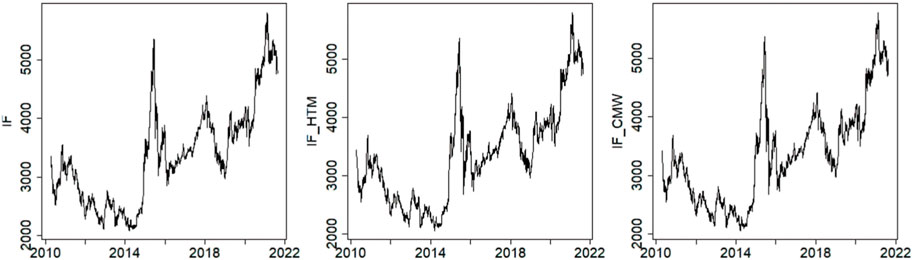
FIGURE 1. CSI 300 price series (IF).

FIGURE 2

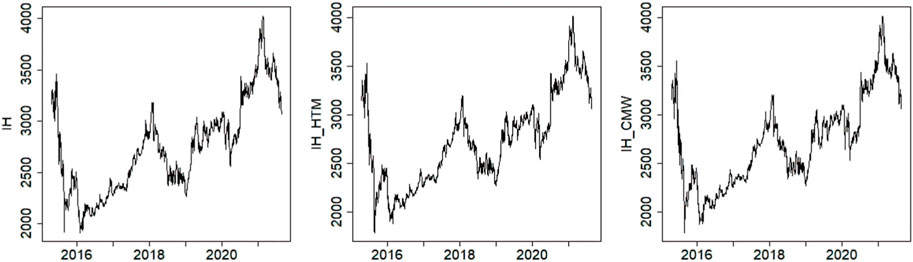
FIGURE 2. SSE 50 price series (IH).

FIGURE 3

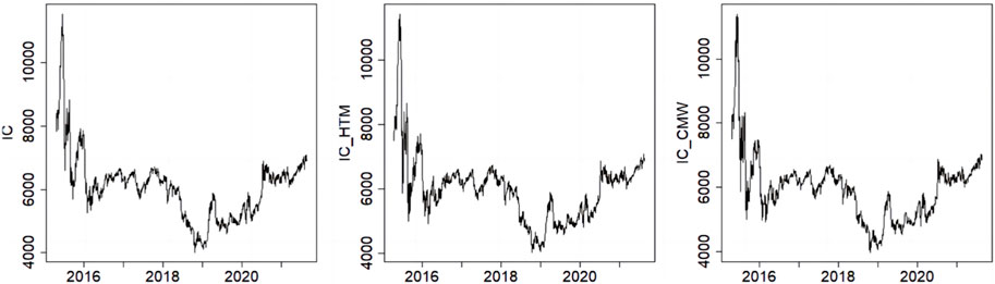
FIGURE 3. CSI 500 price series.

FIGURE 4

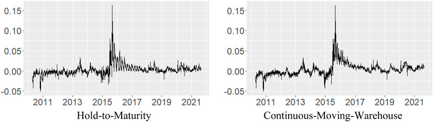
FIGURE 4. Rate of CSI 300 forward discount.

FIGURE 5

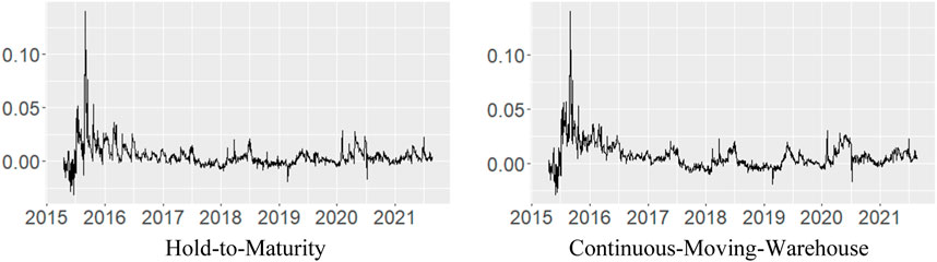
FIGURE 5. Rate of SSE 50 forward discount.

FIGURE 6

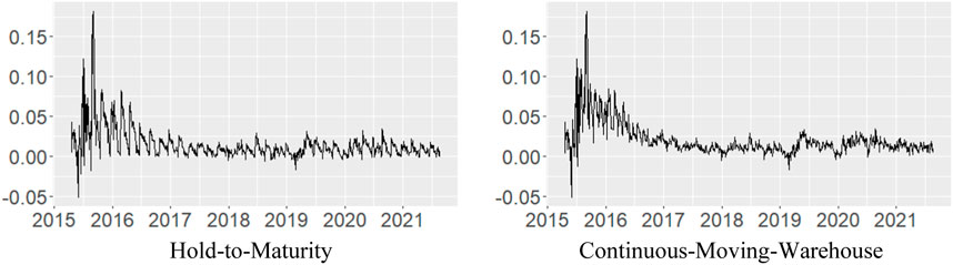
FIGURE 6. Rate of CSI 500 forward discount.

Descriptive statistics and control variable

Table 1 presents the descriptive statistical results of all price return sequences. Firstly, the skewness of all sequences is less than zero, and the kurtosis is greater than 3. Therefore, all return rate sequences can be regarded as distributions that follow a sharp peak with a thick tail and have left bias characteristics. Secondly, in the ADF unit root test, the ADF values of each series were less than −4.58 (1% level threshold), indicating that the price return time series was stable at a 99% confidence level. The KPSS test also supports the inference of data stationarity, and it is feasible to calculate risk spillovers based on stationarity.

TABLE 1

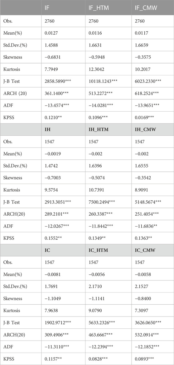
TABLE 1. Descriptive statistics of the return rate of price.

Due to the widespread use of capital cost and inflation rate, stock futures are usually at a discount in the market. The widening basis indicates that the futures price is low and the willingness to sell stocks and recover funds in the future increases. The change of basis can also reflect the change range of futures and spot markets. Therefore, we take the benchmark as the control variable for auxiliary interpretation and include it in the linear regression analysis of the total spillover of hedging indicators. Generally speaking, when the difference between the hedging period and the futures delivery month increases, the basis risk also increases. The rule of thumb suggests that investors should try to choose the delivery month closest to the hedging period but later than that period. Figures 7, 8; Figure 9 describe the basic trends of the three hedging portfolios.

FIGURE 7

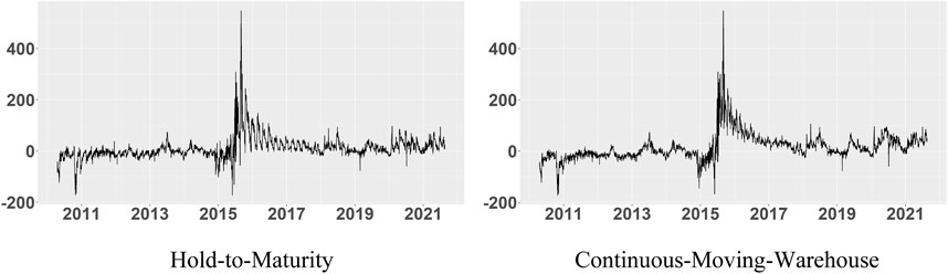
FIGURE 7. Basis risk of CSI 300.

FIGURE 8

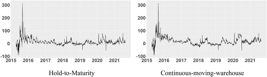
FIGURE 8. Basis risk of SSE 50.

FIGURE 9

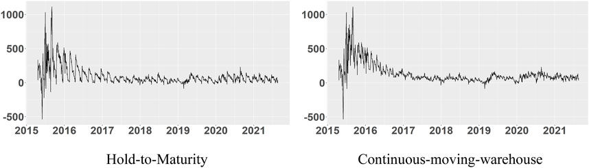
FIGURE 9. Basis risk of CSI 500.

Construction of risk spillovers

The VAR innovations are generally contemporaneously correlated, while the variance decomposition generated by the generalized VaR framework of Koop, Pesaran and Potter (1996) [17] and Pesaran and Shin (1998) [18] (referred to as KPPS) is invariant to the ranking. The connotation of the cross variance shares, or the spillovers, is the fractions of the H-step-ahead error variances in forecasting $x_i$ that are due to shocks to $x_j$, for i, j = 1, 2, . . ., N, such that i $\ne$ j.

Denoting the KPPS H-step-ahead forecast error variance decompositions by ${\theta }_{ij}^g\left(H\right)$, for H = 1, 2, . . ., we have:

${\theta }_{ij}^g\left(H\right)=\frac{{\sigma }_{ij}^{-1}{\sum }_{h=0}^{H-1}{\left(e_i^{\prime }{A}_h\sum e_j\right)}^2}{{\sum }_{h=0}^{H-1}\left(e_i^{\prime }{A}_h\sum A_h^{\prime }{e}_i\right)}(1)$

where $\sum$ is the variance matrix for the error vector $\epsilon$. In addition, $A_h$ is actually the coefficient matrix expressed by the moving average of $x_t$. The moving average representation is $x_t$ = ${\sum }_{i=0}^{\infty }{A}_t{\epsilon }_{t-i}$, where the N × N coefficient matrices $A_i$ obey the recursion $A_i={\mathrm{\Phi }}_1{A}_{i-1}+{\mathrm{\Phi }}_2{A}_{i-2}+\dots +{\mathrm{\Phi }}_p{A}_{i-p}$, with $A_0$ being an N × N identity matrix and with $A_i$ = 0 for i < 0. ${\sigma }_{jj}$ is the standard deviation of the error term for the $j$ th equation, and $e_i$ is the selection vector, with one as the $i$ th element and zeros otherwise. For $i,j\in \left(\mathrm{1,2},\dots ,N\right)$, we can get the variance decomposition matrix ${\theta }^H$, but in the matrix which was explained above, the sum of the elements in each row of the variance de-composition table is not equal to 1: ${\displaystyle \sum _{j=1}^N}{\theta }_{ij}^g\left(H\right)\ne 1$. In order to use the information available in the variance decomposition matrix in the calculation of the spillover, we normalize each entry of the variance decomposition matrix by the row sum as:

${\stackrel{\sim }{\theta }}_{ij}^g\left(H\right)=\frac{{\theta }_{ij}^g\left(H\right)}{{\displaystyle \sum _{j=1}^N}{\theta }_{ij}^g\left(H\right)}(2)$

The standardized matrix contents ${\displaystyle \sum _{j=1}^N}{\stackrel{\sim }{\theta }}_{ij}^g\left(H\right)=1$ and ${\displaystyle \sum _{i,j=1}^N}{\stackrel{\sim }{\theta }}_{ij}^g\left(H\right)=N$.

Basing on the volatility contributions from the KPPS variance decomposition, Diebold and Yilmaz (2012) provided definitions of several risk spillover indicators. The Overall volatility spillover which measures the contribution of spillovers of volatility shocks across four asset classes to the total forecast error variance:

${TS}^H=\frac{{\displaystyle \sum _{i,j=1,i\ne j}^N}{\stackrel{\sim }{\theta }}_{ij}^g\left(H\right)}{{\displaystyle \sum _{i,j=1}^N}{\stackrel{\sim }{\theta }}_{ij}^g\left(H\right)}\bullet 100=\frac{{\displaystyle \sum _{i,j=1,i\ne j}^N}{\stackrel{\sim }{\theta }}_{ij}^g\left(H\right)}{N}\bullet 100(3)$

The propagation spillover (TO) which indicates the information spillover degree of the market $i$ to all other markets $j$ can be constructed based on the prediction error variance matrix constructed above ${\stackrel{\sim }{\theta }}_{ij}^g\left(H\right)$. The TO connectedness can computed as:

$S_{i\to }^g\left(H\right)=\frac{{\displaystyle \sum _{j=1,j\ne i}^N}{\stackrel{\sim }{\theta }}_{ji}^g\left(H\right)}{{\displaystyle \sum _{i,j=1}^N}{\stackrel{\sim }{\theta }}_{ji}^g\left(H\right)}\bullet 100=\frac{{\displaystyle \sum _{j=1,j\ne i}^N}{\stackrel{\sim }{\theta }}_{ji}^g\left(H\right)}{N}\bullet 100(4)$

The acceptance spillover (FROM) indicates the extent to which the market $i$ is subject to information spillover from other markets $j$, and we measure this FROM connectedness as:

$S_{i\leftarrow }^g\left(H\right)=\frac{{\displaystyle \sum _{j=1,j\ne i}^N}{\stackrel{\sim }{\theta }}_{ij}^g\left(H\right)}{{\displaystyle \sum _{i,j=1}^N}{\stackrel{\sim }{\theta }}_{ij}^g\left(H\right)}\bullet 100=\frac{{\displaystyle \sum _{j=1,j\ne i}^N}{\stackrel{\sim }{\theta }}_{ij}^g\left(H\right)}{N}\bullet 100(5)$

Basing on equation (4) and (5), the Net spillover from market $i$ to all other markets $j$ has been defined as:

$S_i^g\left(H\right)=S_{i\to }^g\left(H\right)-S_{i\leftarrow }^g\left(H\right)(6)$

The Net pairwise volatility spillover between markets $i$ and $j$ is simply the difference between the gross volatility shocks transmitted from market $i$ to market $j$ and those transmitted from $j$ to $i$, which we define as:

$S_{ij}^g\left(H\right)=\left(\frac{{\stackrel{\sim }{\theta }}_{ji}^g\left(H\right)}{{\displaystyle \sum _{i,k=1}^N}{\stackrel{\sim }{\theta }}_{ik}^g\left(H\right)}-\frac{{\stackrel{\sim }{\theta }}_{ij}^g\left(H\right)}{{\displaystyle \sum _{j,k=1}^N}{\stackrel{\sim }{\theta }}_{jk}^g\left(H\right)}\right)\bullet 100=\left(\frac{{\stackrel{\sim }{\theta }}_{ji}^g\left(H\right)-{\stackrel{\sim }{\theta }}_{ij}^g\left(H\right)}{N}\right)\bullet 100(7)$

The Net spillover measures the difference between the volatility shocks transmitted to and those received from all other markets. If it is positive, it means that the asset is the net spillover transmitter.

We calculate the hedging ratio according to the optimal hedging ratio summarized by Chen et al (2003) [19], which is defined as:

$h_2=-\frac{C_f^{*}F}{C_{s}S}=-\left[\frac{E\left(R_f\right)}{A{\sigma }_f^2}-\rho \frac{{\sigma }_s}{{\sigma }_f}\right](8)$

Where $E\left(R_f\right)$ is the expected return, $\rho$ is the correlation coefficient, ${\sigma }_s$ is the standard deviation of stock price return $R_s$ and ${\sigma }_f$ is the is the standard deviation of future price return $R_f$. The hedging ratio based on this utility function will conform to the mean variance framework. When the expected return of the futures contract is zero, the minimum variance hedging ratio is equivalent to the optimal mean variance hedging ratio.

We use the method of measuring the hedging effectiveness which proposed by Ederington (1979) [20]:

$H_{\mathrm{e}}=\frac{Var\left(U_t\right)-Var\left(H_t\right)}{Var\left(U_t\right)}(9)$

$Var\left(U_t\right)$ represents the benefit variance when hedging is not performed, and $Var\left(H_t\right)$ represents the benefit variance after hedging. Formula 9 defines hedging effectiveness as the degree of variance reduction between hedging and non-hedging, which is also the part where the price fluctuation risk is reduced by adjusting the futures position in actual operation. The ideal hedging strategy expects that the higher the value, the better.

Results of spillovers

Results in full sample

In this section, we compare the spread of risk spillovers between futures and spot yields using both full sample and rolling sample analyses. We also identify the time periods during which total spillovers exhibit abnormal fluctuations. Our research reveals a clear risk spillover effect between stock futures yield and spot yield. Moreover, the results obtained through rolling sample analysis are better suited to capturing short-term volatility of overall spillover. Notably, during times of significant market impact, the volatility is more pronounced.

Table 2 above displays the spillover effect between the CSI 300 spot and the corresponding futures yield based on the full sample. Using the hold-to-maturity strategy, the overall spillover between the CSI 300 spot and futures yield is 46.57%. From a spillover dissemination perspective, the CSI 300 spot yield has a negative impact on the futures yield. Alternatively, using the continuous-moving-warehouse strategy, the overall spillover between the CSI 300 spot and futures yield is 47.08%. In this case, the spot yield serves as the recipient of spillover information. Using the hold-to-maturity strategy, the overall spillover is 47.07%. Considering the propagation direction, the SSE 50 spot yield has a positive impact on the futures yield. Furthermore, using the hold-to-maturity strategy, the overall spillover between the SSE spot and futures yield is 47.07%. This suggests that the futures yield exhibits a stronger risk spillover effect than the spot yield. In addition, the overall spillovers of the CSI 500 are 45.64% and 46.48%, respectively. Moreover, the futures market exhibits a stronger risk propagation effect under both strategies.

TABLE 2

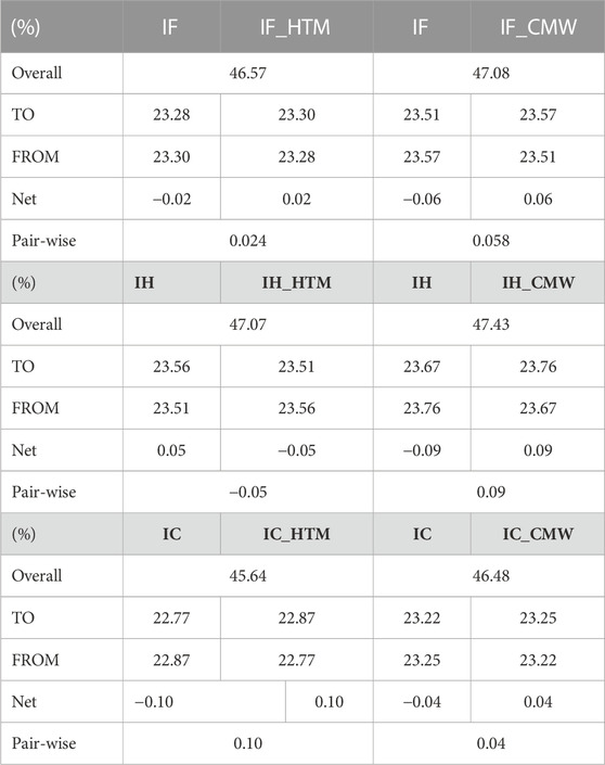
TABLE 2. Spillovers results in full sample.

Results in rolling sample

Furthermore, we calculated the total spillover of six hedge portfolios using a rolling window length of 50 to capture short-term changes in total spillover and obtain continuous results for overall spillover. This approach allowed us to expand the static total spillover obtained from the full sample to dynamic results, which is the core of our research. Figures 10, 11 below illustrate the CSI 300 yield spillover calculated using a rolling window length of 50. Using the hold-to-maturity strategy, the mean total spillover calculated from the rolling sample is 49.25%, while the mean value obtained using the continuous-moving-warehouse strategy is 48.8%. This is in close agreement with the overall spillover obtained from the full sample.

FIGURE 10

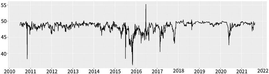
FIGURE 10. Overall spillover of CSI 300 using rolling-window method (Hold-to-Maturity) (%).

FIGURE 11

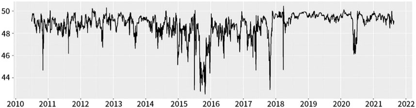
FIGURE 11. Overall spillover of CSI 300 using rolling-window method (Continuous-Moving-Warehouse) (%).

Figures 12, 13 below shows the yield spillover of SSE 50, calculated using the rolling-window method with a window length of 50. When applying the hold-to-maturity strategy, the mean value of the spillover is 48.5%, whereas the mean value under the continuous-moving strategy is 48.8%. From 2015 to 2016, the overall spillover decreased significantly, primarily due to abnormal fluctuations in the spot market.

FIGURE 12

FIGURE 12. Overall spillover of SSE 50 using rolling-window method (Hold-to-Maturity) (%).

FIGURE 13

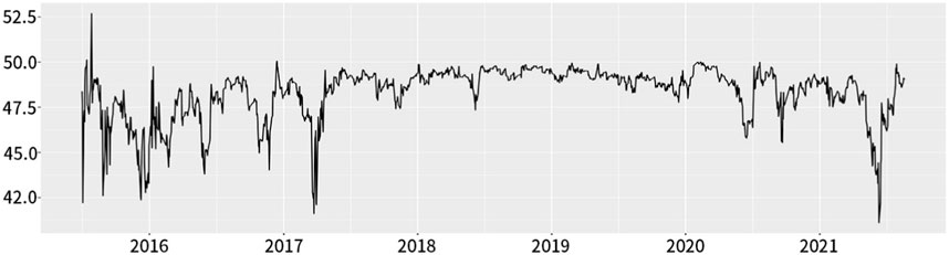
FIGURE 13. Overall spillover of SSE 50 using rolling-window method (Continuous-Moving-Warehouse) (%).

Figures 14, 15 below shows the yield spillover of CSI 500, calculated with a rolling window width of 50. In comparison with CSI 300 and SSE 50, the rolling spillover volatility of CSI 500 is significantly higher throughout the entire sample period. This suggests that the stability of the CSI 500 market is poor and the mutual impact between futures and spot markets is challenging to predict.

FIGURE 14

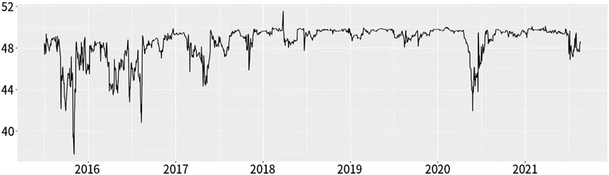
FIGURE 14. Overall spillover of CSI 500 using rolling-window method (Hold-to-Maturity) (%).

FIGURE 15

FIGURE 15. Overall spillover of CSI 500 using rolling-window method (Continuous-Moving-Warehouse) (%).

Linear relationship between overall spillover and hedging indicators

The following section presents the OLS regression results for the overall spillover and hedging ratio. To increase the explanatory power, we include the basis between futures and spot of various varieties as a control variable. For convenience, we expand the overall spillover by a factor of 100 and analysis it without the percent sign. The overall spillover discussed in the following section refers to the expanded index.

Table 3 presents the regression results with overall spillover as the main independent variable and basis as the control variable for the hedging ratio. It should be noted that the overall spillover has never been observed to be zero in history, so the practical significance of a negative intercept is not discussed. The p-values indicate that all coefficient terms are significant at the 1% level.

TABLE 3

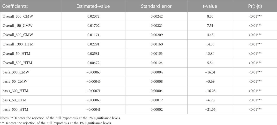
TABLE 3. Overall spillover and hedging ratio regression results.

The results reveal that the overall spillover coefficients of CSI 300, SSE 50, and CSI 500 on the hedge ratio under the continuous-moving-warehouse strategy are 0.0237, 0.0170, and 0.0117, respectively. Under the hold-to-maturity strategy, the coefficients are 0.0229, 0.0258, and 0.0047, respectively. The overall spillover of SSE 50 is the most sensitive to the hedge ratio, while the average spillover sensitivity of CSI 300 is higher. These findings suggest that using CSI 300 futures for hedging is more stable.

The basis directly reflects changes in spot prices. In the equation in the regression, the negative coefficient of the basis indicates that as the basis expands, the spot price gap widens, and the hedge ratio shrinks. This means that as futures prices fall, the size of positions that need to be sold decreases, which affects the arrangement of hedging plans. Regardless of the type of contract, an increase in overall spillover improves the hedging ratio, indicating that risk spillover information between futures and stocks can be reflected in the hedging strategy and help achieve the goal of hedging.

Moving on to the impact of overall spillovers on hedging effectiveness, we should note that the hedge effectiveness of the six portfolios is calculated according to Formula 9. We use a linear regression model to examine the direction and sensitivity of the spillovers to hedging effectiveness.

Table 4 presents the coefficients of overall spillovers of CSI 300, SSE 50, and CSI 500 on the effectiveness of hedging under the continuous-moving-warehouse and hold-to-maturity strategies. The coefficients for the continuous-moving-warehouse strategy are 0.0223, 0.0309, and 0.0240, respectively, while under the hold-to-maturity strategy, the coefficients are 0.0231, 0.0268, and 0.0170, respectively. All coefficients are significant at the 1% level, which is consistent with the regression results in Table 3. The basis samples have a negative change relationship with hedging effectiveness across the board.

TABLE 4

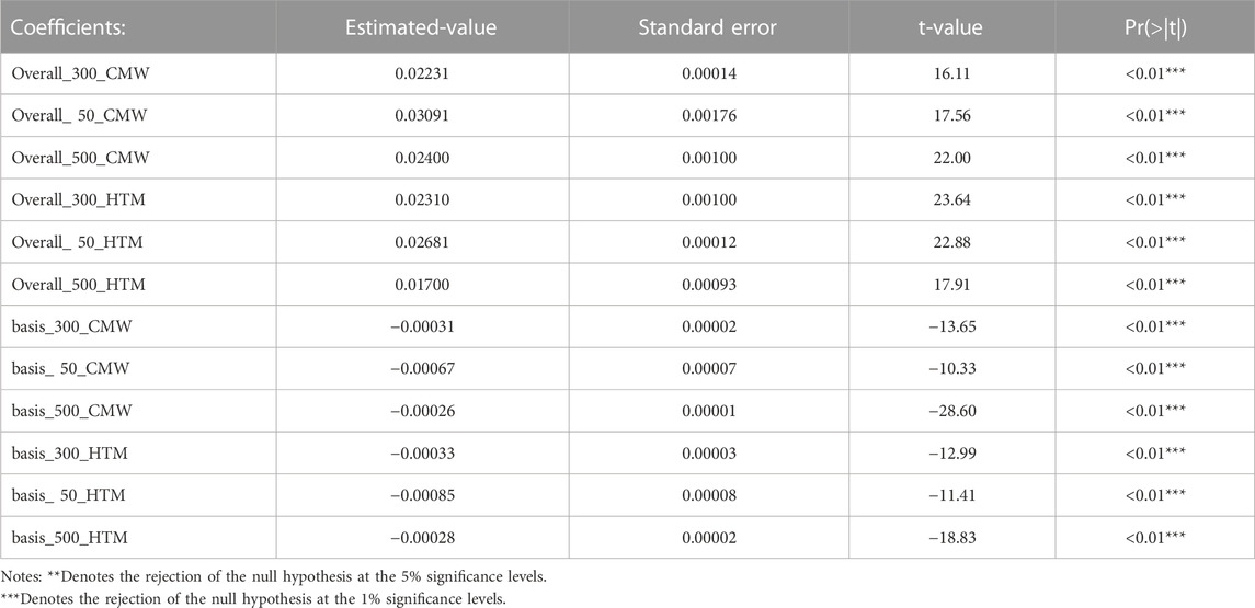
TABLE 4. Overall spillover and hedging effectiveness regression results.

The average value of the overall spillover coefficient is higher for the continuous-moving-warehouse strategy than for the hold-to-maturity strategy. This could be due to the higher liquidity of futures contracts required for the continuous-moving-warehouse strategy, which helps to avoid the loss of hedging effectiveness caused by the gradual decline of contract liquidity. From the perspective of the variety of futures contracts, the coefficient of SSE 50 overall spillover is more sensitive to both the hedging ratio and effectiveness. The results show that as the overall spillover of the futures and spot markets increases, the hedging effectiveness also increases. This is because the transmission of risk spillover information expands, making the pace of price changes of futures and spot assets closer. As a result, the price volatility reduced by hedging is greater, and investors can obtain better hedging effectiveness.

In the next section, the OLS model is used to measure the regression result between the overall spillover and the total cost of hedging. To begin with, the total cost will have two parts: the amount paid to buy shares and the interest of financing the position. Hull (2009) defined the hedging cost as the present value of the accumulated net cost of buying and selling stocks [21]. The standard deviation of the cost of hedging can be reduced by shortening the rebalancing period.

Table 5 presents the regression results of all the overall spillover samples on the total hedging cost. Unlike Tables 3, 4, we did not introduce the basis in the regression analysis of CSI 300 in order to retain the model results with a higher R-squared. The coefficients of the overall spillovers of CSI 300, SSE 50, and CSI 500 are 114, 58.72, and 46.10, respectively, in the continuous-moving-warehouse strategy. In the hold-to-maturity strategy, the coefficients are 117.73, 74.71, and 55.24, respectively. All variables are significant at the 1% level.

TABLE 5

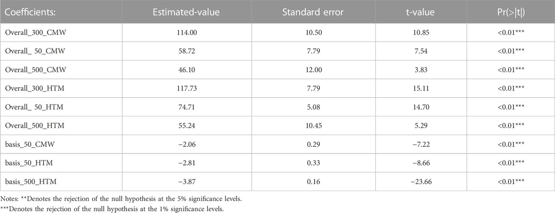
TABLE 5. Overall spillover and hedging cost regression results.

From the results, we observe that all the overall spillover coefficients have positive relationships with the hedging cost. As the overall spillover increases, the hedging cost also increases. When combined with Table 5, we can see that the enhancement of risk spillover makes the hedging ratio gradually expand to 1, which directly leads to an increase in the futures positions that should be sold. This is one of the reasons for the increase in hedging costs.

Moreover, since daily position adjustments cause the futures margin to constantly change, excessive trading frequency will also lead to the accumulation of management costs, handling fees, trading commissions, stamp duty, and so on. Comparing the time of conversion contracts, we see that the trading time of continuous position change is the third Friday of each month, which is more regular than the hold-to-maturity strategy and has better liquidity. When the comparison coefficient is large, we can see that the total spillover in the continuous position shifting strategy is less sensitive to the hedging cost than the hold-to-maturity strategy. In other words, as the overall spillover of the futures and spot markets increases, the increase in hedging costs for continuous position shifting is lower than for hold-to-maturity. This is conducive to maintaining the stability of hedging costs and optimizing the liquidity management of capital lending to achieve the hedging objectives.

Robustness

In the end, we aim to discuss the robustness of the calculation methods under different measurement parameters. To ensure the credibility of our conclusions, we assume that the risk spillover should not be significantly affected by the rolling window length, and the measurement of the hedging effect of the total spillover index should not be influenced by the adjustment frequency of futures contracts. We adjusted the period on a daily, weekly, and every 3-week term and recalculated the corresponding hedge effectiveness.

Firstly, Figure 16 illustrate the robustness of CSI300, SSE 50, and CSI 500 samples concerning the hedging periods. Compared to CSI 300 and SSE 50, the hedging effectiveness of CSI 500 fluctuates considerably. This observation suggests that the first two contracts may be more suitable as hedging tools for spot stocks than CSI 500. We found that only the hedging effectiveness sample of CSI 500 with a period of 15 experienced a slight decline from June to August 2015 to July 2016, while the trend of other samples remained consistent under different hedging periods. This finding emphasizes the basic trend rather than the specific effectiveness, indicating that the selection of the hedging period does not affect the persistence of the spillover on the transmission of hedging policy information.

FIGURE 16

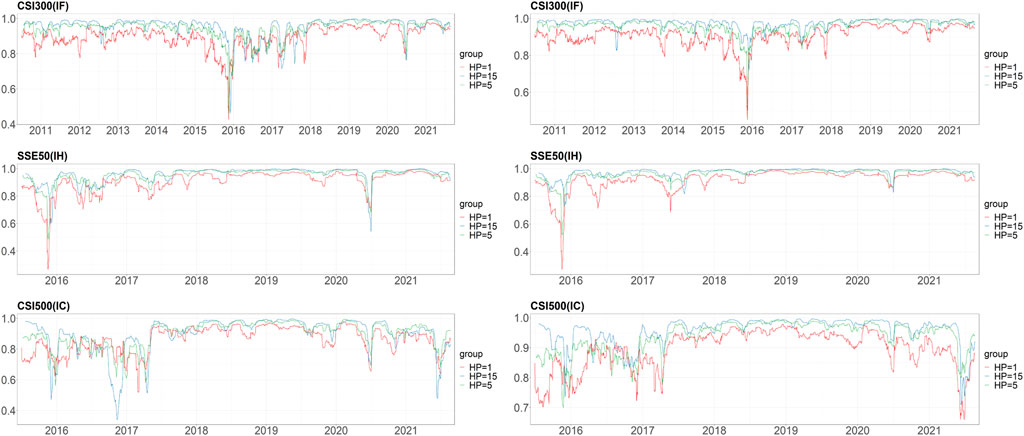
FIGURE 16. Hedge effectiveness in different hedging periods (left for HTM and right for CMW).

Secondly, we examine the sensitivity of hedging effectiveness to the choice of steps of forecast error variance decomposition separately under the two strategies. The method involves changing the VaR steps and examining whether the superimposed trends of hedging effectiveness are close. As shown in Figure 17, which correspond to the hold-to-maturity strategy, we find that the CSI 500 is not as volatile as the CSI 300 during the “China Stock Market Crash” due to its own volatility in the spot market. After the extreme period, the effectiveness results calculated using different parameters tend to be consistent, and the influence of extreme events will be basically the same under different window length. Moreover, the effectiveness of CSI 500 is slightly greater than that of CSI 300 and SSE 50, whether it is the fluctuation of a single series or the difference in the trend of the series under different windows. This is due to the fact that the effectiveness and liquidity of CSI 500s spot market is inferior to the former two, and the practicability of hedging with this kind of future is uncertain. Overall, we can see from Figure 17 that adjusting the length of the scrolling window does not affect the measurement of hedge effectiveness. Therefore, we believe that the length of the rolling window is not an objective factor affecting the hedging effectiveness measurement.

FIGURE 17

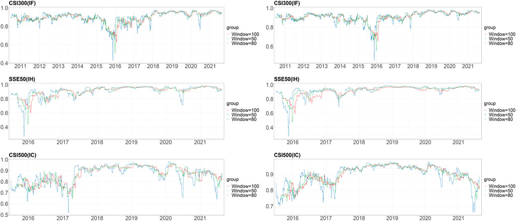
FIGURE 17. Hedge effectiveness in different steps of forecast error variance decomposition (left for HTM and right for CMW).

Thirdly, we measured whether the unit window length has a special impact on the overall spillover trend. This parameter is the sample size taken at a single time when we scroll to grab the overall spillover. Specifically, we changed this length to check whether it would affect the overall spillover index. As shown in Figure 18, the trends of the overall spillovers of CSI 300 and SSE 50, which are under the hold-to-maturity, remain basically the same when the step size was changed from 50 to 60 to 70. Only the overall spillover of CSI 500 fluctuated slightly more than the first two types of results during the extreme stock disaster, but the mean of their extreme differences does not exceed 1.8%. The average value of the overall overflow of the above different parameters is close to the value of the original sample.

FIGURE 18

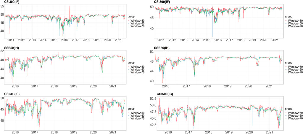
FIGURE 18. Overall spillover in different rolling windows (left for HTM and right for CMW).

In general, when measuring the overall spillover index and hedging effectiveness of the above samples, the measurement methods used are not subject to the qualitative or quantitative impact of the above three factors. Under this method, the analysis process that examines the significant relationship between the risk spillover effect of the futures and spot market and the hedging strategy can be repeated.

Conclusion

We measure risk spillovers for six stock index hedged portfolios with different strategies and categories and linearly regress the overall spillovers against the hedge ratio, hedge effectiveness, and total hedging costs. To begin with, it shows that there are significant risk spillover effects between China’s stock market and futures markets, for the CSI 300 and CSI 500 markets, the number of companies in these two market sizes is larger than that of the SSE 50, which can better illustrate the general performance of the Chinese market. Overall, China’s stock market is more susceptible to the impact of futures prices. Therefore, we believe that when evaluating the overall performance of the stock market, changes in the futures market should be considered and mining risk information from futures price changes to provide early warning for the stock market. For example, when malicious speculation occurs in the futures market, we have reason to believe that this risk will spread to the stock market and cause losses to stock investors. For SSE 50, the performance of stocks is more active and stronger than futures prices. This is because the companies selected by SSE 50 are the most influential and outstanding companies in the Chinese stock market. When investors invest in the SSE 50 Index, they focus more on the profitability and growth of these companies themselves, rather than speculation in the futures market. Therefore, the growth of the stock price itself has more impact than the futures market’s prediction of future investment sentiment.

Furthermore, we confirm that there is a significant positive relationship between the overall risk spillovers in the stock futures spot market and hedging ratios, hedging effectiveness, and hedging costs. When the risk spillover relationship between the futures and spot markets increases, that is, the risk fluctuations in the two markets are relatively synchronized, it will help achieve more effective hedging activities. This relationship holds during periods of extreme stock market declines, and hedging measures for more liquid portfolios are more sensitive to aggregate spillovers. The risk spillover used in this article can be regarded as a quantitative tool to describe the relationship between time series based on VAR and variance error contribution. Compared with multivariate linear relationships, it has the characteristics of mining richer and more accurate information. Therefore, the conclusion we found that using overall risk spillover as a predictive hedging strategy is more practical, that is, using the overall risk spillover as a factor and basis to help traders adjust the stocks used for hedging based on Futures positions. Briefly, when the overall spillover effect increases, the selling position can be increased according to the hedging ratio and the sensitivity of the total spillover effect to achieve a higher hedging effect.

Data availability statement

Publicly available datasets were analyzed in this study. This data can be found here: www.wind.com.cn.

Author contributions

KS: Writing–original draft. JG: Writing–review and editing.

Funding

The author(s) declare financial support was received for the research, authorship, and/or publication of this article. This study was funded by National Social Sciences Funds (20BTJO15).

Acknowledgments

All authors thank the graduate school and School of economics and management of Northeast China Normal University and the National Social Science Foundation of China for their support for this study.

Conflict of interest

The authors declare that the research was conducted in the absence of any commercial or financial relationships that could be construed as a potential conflict of interest.

Publisher’s note

All claims expressed in this article are solely those of the authors and do not necessarily represent those of their affiliated organizations, or those of the publisher, the editors and the reviewers. Any product that may be evaluated in this article, or claim that may be made by its manufacturer, is not guaranteed or endorsed by the publisher.

References

1. Basher SA, Sadorsky P. Hedging emerging market stock prices with oil, gold, VIX, and bonds: a comparison between DCC, ADCC and GO-GARCH. Energy Econ (2016) 54:235–47. doi:10.1016/j.eneco.2015.11.022

CrossRef Full Text | Google Scholar

2. Kang SH, McIver R, Yoon S-M. Dynamic spillover effects among crude oil, precious metal, and agricultural commodity futures markets. Energ Econ (2017) 62:19–32. doi:10.1016/j.eneco.2016.12.011

CrossRef Full Text | Google Scholar

3. Wang G-J, Xie C, He K, Stanley HE. Extreme risk spillover network: application to financial institutions. Quant Finance (2017) 17:1417–33. doi:10.1080/14697688.2016.1272762

CrossRef Full Text | Google Scholar

4. Al-Yahyaee KH, Mensi W, Al-Jarrah IMW, Hamdi A, Kang SH. Volatility forecasting, downside risk, and diversification benefits of Bitcoin and oil and international commodity markets: a comparative analysis with yellow metal. North american journal economics finance (2019) 49:104–20. doi:10.1016/j.najef.2019.04.001

CrossRef Full Text | Google Scholar

5. Kocenda E, Moravcova M. Exchange rate comovements, hedging and volatility spillovers on new EU forex markets. Journal international financial markets institutions money (2019) 58:42–64. doi:10.1016/j.intfin.2018.09.009

CrossRef Full Text | Google Scholar

6. Diebold FX, Yilmaz K. Measuring financial asset return and volatility spillovers, with application to global equity markets. Economic journal (2009) 119:158–71. doi:10.1111/j.1468-0297.2008.02208.x

CrossRef Full Text | Google Scholar

7. Diebold FX, Yilmaz K. Better to give than to receive: predictive directional measurement of volatility spillovers. Int J Forecast (2012) 28:57–66. doi:10.1016/j.ijforecast.2011.02.006

CrossRef Full Text | Google Scholar

8. Diebold FX, Yilmaz K. On the network topology of variance decompositions: measuring the connectedness of financial firms. J Econom (2014) 182:119–34. doi:10.1016/j.jeconom.2014.04.012

CrossRef Full Text | Google Scholar

9. Barunik J, Krehlik T. Measuring the frequency dynamics of financial connectedness and systemic risk. Journal financial econometrics (2018) 16:271–96. doi:10.1093/jjfinec/nby001

CrossRef Full Text | Google Scholar

10. Antonakakis N, Cunado J, Filis G, Gabauer D, de Gracia FP. Oil volatility, oil and gas firms and portfolio diversification. Energ Econ (2018) 70:499–515. doi:10.1016/j.eneco.2018.01.023

CrossRef Full Text | Google Scholar

11. Engle R. Dynamic conditional correlation: a simple class of multivariate generalized autoregressive conditional heteroskedasticity models. Journal business economic statistics (2002) 20:339–50. doi:10.1198/073500102288618487

CrossRef Full Text | Google Scholar

12. Akhtaruzzaman M, Boubaker S, Sensoy A. Financial contagion during COVID-19 crisis. Financ Res Lett (2021) 38:101604. doi:10.1016/j.frl.2020.101604

PubMed Abstract | CrossRef Full Text | Google Scholar

13. Lau CKM, Bilgin MH. Hedging with Chinese aluminum futures: international evidence with return and volatility spillover indices under structural breaks. EMERGING MARKETS FINANCE AND TRADE (2013) 49:37–48. doi:10.2753/REE1540-496X4901S103

CrossRef Full Text | Google Scholar

14. Yarovaya L, Brzeszczynski J, Lau CKM. Intra- and inter-regional return and volatility spillovers across emerging and developed markets: evidence from stock indices and stock index futures. INTERNATIONAL REVIEW FINANCIAL ANALYSIS (2016) 43:96–114. doi:10.1016/j.irfa.2015.09.004

CrossRef Full Text | Google Scholar

15. Lai YH, Wang YC. Jump-dependent model for optimal index futures hedging in five major asian stock markets. EMERGING MARKETS FINANCE AND TRADE (2016) 52:786–96. doi:10.1080/1540496X.2015.1117875

CrossRef Full Text | Google Scholar

16. Magkonis G, Tsouknidis DA. Dynamic spillover effects across petroleum spot and futures volatilities, trading volume and open interest. INTERNATIONAL REVIEW FINANCIAL ANALYSIS (2017) 52:104–18. doi:10.1016/j.irfa.2017.05.005

CrossRef Full Text | Google Scholar

17. Koop G, Pesaran MH, Potter SM. Impulse response analysis in nonlinear multivariate models. J Econom (1996) 74:119–47. doi:10.1016/0304-4076(95)01753-4

CrossRef Full Text | Google Scholar

18. Pesaran HH, Shin Y. Generalized impulse response analysis in linear multivariate models. Econ Lett (1998) 58:17–29. doi:10.1016/S0165-1765(97)00214-0

CrossRef Full Text | Google Scholar

19. Chen S-S, Lee C, Shrestha K. Futures hedge ratios: a review. Q Rev Econ Finance (2003) 43:433–65. doi:10.1016/S1062-9769(02)00191-6

CrossRef Full Text | Google Scholar

20. Ederington LH. The hedging performance of the new futures markets. J Finance (1979) 34:157–70. doi:10.1111/j.1540-6261.1979.tb02077.x

CrossRef Full Text | Google Scholar

21. Hull JC. Solutions manual options, futures, and other derivatives. London, England: Pearson Education (2009).

Google Scholar