Dynamic displacement estimation of structures using one-dimensional convolutional neural network

For large infrastructures, dynamic displacement measurement in structures is an essential topic. However, limitations imposed by the installation location of the displacement sensor can lead to measurement difficulties. Accelerometers are characterized by easy installation, good stability and high sensitivity. For this regard, this paper proposes a structural dynamic displacement estimation method based on a one-dimensional convolutional neural network and acceleration data. It models the complex relationship between acceleration signals and dynamic displacement information. In order to verify the reliability of the proposed method, a finite element-based frame structure was created. Accelerations and displacements were collected for each node of the frame model under seismic response. Then, a dynamic displacement estimation dataset is constructed using the acceleration time series signal as features and the displacement signal at a certain moment as target. In addition, a typical neural network was used for a comparative study. The results indicated that the error of the neural network model in the dynamic displacement estimation task was 9.52 times higher than that of the one-dimensional convolutional neural network model. Meanwhile, the proposed modelling scheme has stronger noise immunity. In order to validate the utility of the proposed method, data from a real frame structure was collected. The test results showed that the proposed method has a mean square error of only 5.097 in the real dynamic displacement estimation task, which meets the engineering needs. Afterwards, the outputs of each layer in the dynamic displacement estimation model are visualized to emphasize the displacement calculation process of the convolutional neural network.

1 Introduction

With the development of structural health monitoring, the safety of some structures, such as high-rise buildings [1, 2], bridges [3, 4], and rapid transit [5, 6], has gradually attracted public attention. These structures may be affected by natural disasters such as typhoons and earthquakes. These natural disasters could cause structural damage and even lead to major accidents. Therefore, these structures are usually equipped with structural health monitoring systems and a large number of sensors [7–10] are placed to monitor the safety of the structure. The most common sensors used in structural safety monitoring are accelerometers, fiber-optic gratings, strain gauges, displacement gauges, and so on. However, structural displacement monitoring has been a challenge in the monitoring field. Due to the limitation of structural space, it is sometimes difficult to find suitable locations for sensor installation, such as dynamic displacement detection in bridges. Even if there is enough space in the structure to install sensors, only relative displacement can be measured. Acceleration is easier to monitor than displacement. Furthermore, acceleration sensors can be connected directly to the test point. In addition, acceleration sensors are small and convenient and do not require a large installation space, so acceleration monitoring is easy to implement in engineering applications.

Despite the many difficulties in displacement monitoring, many innovative monitoring methods based on certain sensors have been proposed, such as lasers [11, 12], cameras [13, 14], radar [15], and global positioning systems [16]. These methods have been widely used in real structures, and even some sophisticated measurement devices such as laser displacement sensors, total stations, and millimeter wave radars have emerged. However, these displacement measurement devices still require a large installation space. They can only measure the relative displacement of the structure, and the actual displacement of the structure is difficult to measure. For bridge deflection measurement, it is impossible to build scaffolding on both sides of the bridge to install the sensors. Therefore, the installation space is a key issue that restricts the displacement measurement. In addition, there are many indirect monitoring methods based on acceleration data. Theoretically, the displacement signal can be obtained by double integration of the acceleration signal. The monitoring of acceleration signals is very easy to achieve, so some dynamic displacement measurement methods based on acceleration signals have been proposed. However, these methods may result in a continuous error trend in the displacement signal. Various algorithms for eliminating the error trend [17–20] have been extensively studied. The methods for removing the error trend are mainly classified into three types: time-domain integration, filtering, and frequency-domain integration. These integration methods are fixed signal processing methods that are not able to adapt to changes in the environment and uncertainty in the data. In complex and dynamic environments, these methods may not be able to adapt and process data efficiently. They are mostly used for linear signal processing and have limited ability to deal with nonlinear problems. However, many phenomena in engineering are non-linear issues [21]. Machine learning methods are better able to cope with nonlinear problems and improve performance by learning the nonlinear relationships of the data. Compared to machine learning, they have some limitations in terms of data dependency, feature design, adaptivity and non-linear problem handling. In addition, some neural networks are devoted to address multimodal functional synchronization [22, 23] and communication security [24]. Machine learning methods are more flexible in dealing with different types of data and can automatically learn features and patterns from data, making them more applicable in dealing with complex and uncertainty-prone problems.

In recent years, Convolutional Neural Network (CNN) has made great achievements in the field of object recognition. It is widely used in various fields, such as image recognition [25–28], medical diagnosis [29, 30], traffic safety [31, 32], crack detection [33, 34], pedestrian identification [35], and bolt loosening monitoring [36, 37]. These research results show that convolutional neural networks can accurately model numerous complex systems relying on big data. Li et al. accurately identified concrete surface cracks using a semantic segmentation algorithm based on convolutional neural networks [38, 39]. According to the semantic recognition results, they extracted the crack parameters and analyzed the fractal characteristics of the surface cracks from different specimens using image processing techniques. Zhang et al. used a convolutional neural network to process the time-frequency features of the seismic response, which were subsequently input into a dynamic network to complete the signal classification [40]. The convolutional neural network can deeply analyze the two-dimensional time-frequency features, and the dynamic network further improves the efficiency of signal processing [41]. All of these monitoring methods are based on two-dimensional convolutional neural networks, but one-dimensional convolutional neural networks [42, 43] also have great advantages in data processing. In recent years, convolutional neural networks have achieved remarkable results in the field of image processing. Consequently, the integration of CNNs and machine vision has become widely prevalent. However, when it comes to extracting localized features in image processing, the commonly employed approach is the utilization of two-dimensional CNNs. One-dimensional convolutional neural networks are commonly used to process one-dimensional signals, such as acceleration signals. Two-dimensional convolutional neural networks cannot directly process one-dimensional signals. Of course, one-dimensional signals can be converted into two-dimensional features, such as time-frequency features for processing by two-dimensional convolutional neural networks. However, one-dimensional convolutional neural networks can directly extract features from one-dimensional signals without additional conversion steps to achieve good recognition results. In addition, convolutional neural networks have the ability of autonomous learning. There is a simple integral relationship between acceleration and displacement at the same point. Although there is a trend term, the convolutional neural network has a strong learning ability to learn how to remove the trend term. In addition, the convolutional neural network has the ability to extract data features and optimize them without human intervention. Convolutional neural networks are very effective in processing data.

In this paper, a new method for estimating dynamic displacements of structures using one-dimensional convolutional neural networks and acceleration is presented. The method is used to estimate the dynamic displacement of a three-layer finite element model and a three-layer steel frame. A typical neural network algorithm provides a reference for the proposed CNN method. Section 2 describes the neural network and convolutional neural network used in this paper. A finite element model is designed in Section 3. Under the effect of Wenchuan earthquake wave, the acceleration signal and displacement signal of each node of the model are collected to form a dataset. The data set is divided into training set, validation set and test set. The training and validation sets are fed into the neural network and the proposed convolutional neural network. To validate the noise resistance of the proposed method, four noise levels (i.e., 10%, 20%, 30%, and 40%) are added to the acceleration signals to examine the robustness of the CNN to noisy data. These data were directly fed into the training model, which was trained by the noise-free dataset. The results show that the convolutional neural network is robust to noise. In Section 4, a three-layer steel frame is constructed and the acceleration signals and displacement signals of the nodes of the frame are collected by acceleration sensors and displacement sensors. The training and validation sets are fed into the proposed convolutional neural network. The results show that the mean square error (MSE) of the displacement estimation is 5.097, which can meet the engineering needs. Subsequently, the output of each layer is visualized to understand how the convolutional neural network processes the data. Section 5 discusses the article. Section 6 summarizes the article.

2 Methodology

This paper presents a dynamic displacement estimation method based on a one-dimensional convolutional neural network and acceleration signals. The method uses acceleration signals and an estimation model trained by a convolutional neural network to estimate the dynamic displacement of the structure. The estimation results of the neural network method can be used as a reference for the proposed convolutional neural network method. The following section describes the neural network and convolutional neural network in detail. In this paper, a workstation is used to train the model and computational frameworks such as TENSORFLOW and KERAS are applied.

2.1 Neural network

Neural network algorithms are generated by modelling the working of human neurons. A neural network generally consists of an input layer, a hidden layer, and an output layer, as shown in Figure 1. Sometimes, a neural network may have more than one hidden layer. In a fully connected neural network, neurons between two neighboring layers are connected exactly in pairs. The weights refer to the strength or amplitude of the connection between two neurons. During training, these connection weights are updated until the global error of the network approaches a minimum. In the parameter update calculation, this is typically done using a gradient descent algorithm. The key to the gradient descent algorithm is the calculation of the gradient, which tells us how to update the parameters to minimize the loss function. Gradient descent algorithms generally include Batch Gradient Descent, Stochastic Gradient Descent and Mini-Batch Gradient Descent [44]. They differ in the number of samples used each time the parameters are updated. Gradient descent algorithms have the advantage of being simple to implement and can be used to optimize a variety of loss functions.

FIGURE 1

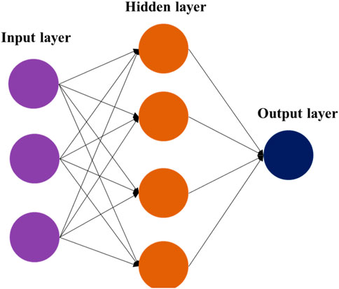
FIGURE 1. Neural network diagram.

The neural network used in this paper consists of one input layer, two hidden layers and one output layer, as shown in Tabel 1. The number of neurons in the input layer is 50, the number of neurons in the first hidden layer is 30, the number of neurons in the second hidden layer is 20, and the number of neurons in the output layer is 1. In general, the raw data usually has highly dense features, and the complex features can be transformed into sparse features. This can enhance the robustness of the features. Therefore, introducing an activation function in the neural network can improve the data sparsity. However, a large proportion of sparsity can destroy the characteristics of the data and affect the learning effect of the neural network. The sparsity ratio of human brain is 95%. Due to the property of Rectified Linear Unit (ReLU) (negative output of x is 0), Rectified Linear Unit (ReLU) can be generated for alternate networks. ReLU is shown in Figure 2. ReLU is a nonlinear activation function that helps the neural network model to learn nonlinear relationships. This is important for solving complex problems and fitting nonlinear data. In addition, the output of ReLU is 0 when the input value is less than 0. This means that there will not be any negative signals passed to the next layer of neurons. This sparse activation can help the network learn more robust feature representations and reduce redundancy between features [45]. Compared to other activation functions such as sigmoid and tanh which have small gradients over positive intervals, ReLU has constant gradients over positive intervals, reducing the problem of gradient vanishing and facilitating the training of the network.

TABLE 1

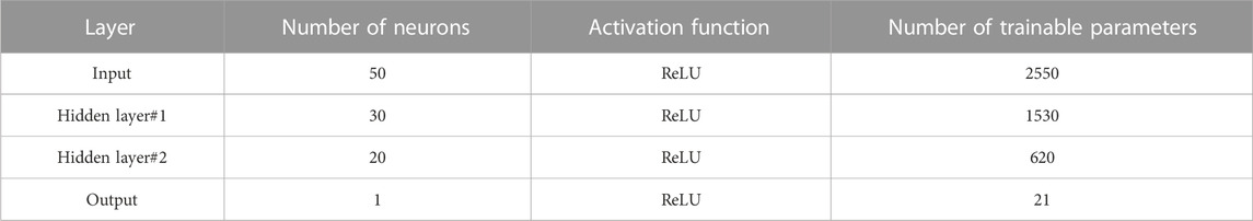
TABLE 1. Architecture of the neural network.

FIGURE 2

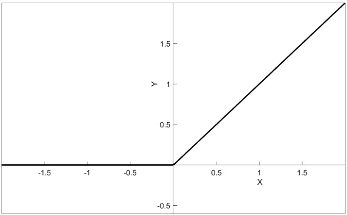
FIGURE 2. Activation function.

The loss function is mainly used to measure the difference between the predicted value and the actual value. When the predicted value is closer to the actual value, the value of the loss function is smaller. When the predicted value is closer to the actual value, the value of the loss function is smaller. In neural networks, the loss function is the mean square error (MSE), which is often used in regression problems. The MSE can be calculated as the square of the difference between the actual value and the predicted value. The formula is as follows:

$MSE=\frac{1}{n}{\displaystyle \sum _{i=1}^n}{\left({actual}_i-{predicted}_i\right)}^2(1)$

where n is the number of samples; actual is the actual value; predicted is the predicted value; i is the i-th sample. In order to comprehensively assess the impact of noise on the proposed method, three evaluation metrics such as Mean Absolute Error (MAE), Mean Absolute Percentage Error (MAPE), and R² are also calculated.

$MAE=\frac{1}{n}{\displaystyle \sum _{i=1}^n}\left|{actual}_i-{predicted}_i\right|(2)$

$MAPE=\frac{100\%}{n}{\displaystyle \sum _{i=1}^n}\left|\frac{{actual}_i-{predicted}_i}{{actual}_i}\right|(3)$

$R^2=1-\frac{{\displaystyle \sum _{i=1}^n}{\left({actual}_i-{predicted}_i\right)}^2}{{\displaystyle \sum _{i=1}^n}{\left({actual}_i-mean\right)}^2}(4)$

where mean represents the mean value of the real sample.

2.2 Convolutional neural network

The major difference between convolutional neural networks and ordinary neural networks is the convolution operation. To illustrate the advantages of convolutional neural networks, the proposed convolutional neural network uses the same activation function and loss function as the fully connected neural network. The architecture of the convolutional neural network is different from the fully connected neural network. Convolutional neural network contains convolutional layer, maximum pooling layer, flat layer and dense (fully connected) layer. Each neuron in a neural network is connected to all the previous layers of neurons, which leads to a large increase in the number of parameters. Whereas in CNN only the inputs that are within the range of the convolutional kernel will be selected for connection, which reduces the number of parameters and increases the computational efficiency. The detailed parameters of the convolutional neural network are shown in Table 2.

TABLE 2

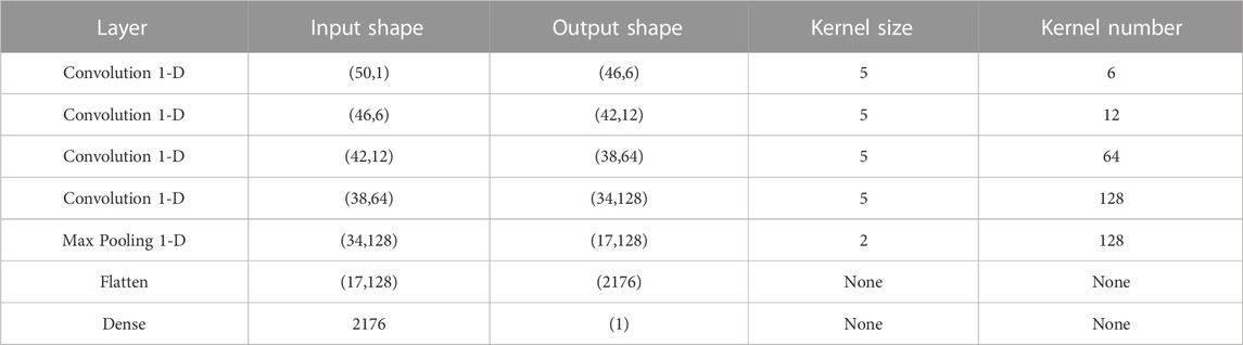
TABLE 2. The parameters of the convolutional neural network.

2.2.1 Convolutional layer

The convolutional layer is an important part of a convolutional neural network. The convolutional kernel extracts feature from the input data. CNNs use the convolutional kernel to perform sliding window operations on the input data, reducing the number of parameters in the network by means of parameter sharing. This makes CNNs more efficient in processing data with spatial and temporal relationships and allows spatially localized features to be extracted [46]. The convolution operation (⊗) starts from the top left corner of the input data. The parameters of the convolution kernel are multiplied with the parameters of the overlay region. The product values are added together as the output of the convolution operation. The convolution kernel is then shifted one element to the right or down (stride is 1) for the next convolution. The initial parameters of the convolution kernel are randomly generated. During the training process, the parameters of the convolution kernel are updated until the end of training. An example of a convolution operation is shown in Figure 3.

FIGURE 3

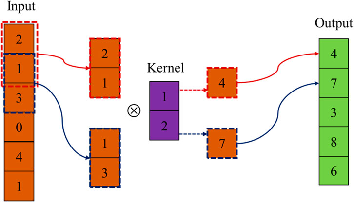
FIGURE 3. Example of convolutional operation.

2.2.2 Pooling layer

The pooling layer, also known as the down sampling layer, is mainly used to reduce the size of the feature data. CNNs use a pooling layer to reduce the spatial size of the feature map, to extract the positional information of the features and at the same time to preserve the most salient features in the feature map. Similar to convolutional layers, pooling layers allow for parameter sharing. This means that pooling operations performed in a local region use the same parameters, which can effectively reduce the number of parameters in the network and improve the computational efficiency of the model. In addition, like convolutional layers, pooling layers have a kernel. However, the pooling kernel does not contain any parameters. The most common pooling operation is maximum pooling. By selecting the maximum value within a local region, maximum pooling captures the most salient features. It is very effective in highlighting the most important and active features in the data [47]. An example of the max pooling operation is shown in Figure 4. For mean pooling, the input features can be smoothed by averaging them to reduce noise and redundant information.

FIGURE 4

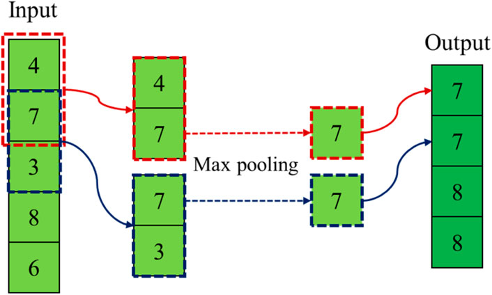
FIGURE 4. Example of pooling operation.

2.2.3 Flatten layer

In this paper, the input data to the network is one-dimensional data. One convolutional kernel in the convolutional layer is convolved with the input data to generate one-dimensional data and multiple convolutional kernels are convolved with the input data to generate multidimensional data. The input data of the dense (fully connected) layer must be one-dimensional data. Therefore, the multidimensional data is transformed into one-dimensional data by the Flatten layer. The Flatten layer transforms the multidimensional input data into one-dimensional vectors, allowing the subsequent fully-connected layer to process the entire input. It is useful for processing multidimensional data, and after converting the input data into a one-dimensional form, the common neural network architecture can be used in the fully connected layer.

3 Numerical simulation

3.1 Dataset generation

The finite element model was created by ABAQUS. The model is a three-storey frame structure with a storey height of 4,500 mm and a span of 7,200 mm. The beams and columns are made of Q235 steel. The seismic intensity is 8°. The finite element model and node numbers are shown in Figure 5.

FIGURE 5

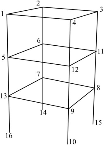
FIGURE 5. The finite element model and node number.

The Wenchuan seismic waves are input into the finite element model and then the acceleration and displacement signals of twelve nodes (1, 2, 3, 4, 5, 6, 7, 8, 9, 11, 12 and 13) are collected. The acceleration signals with a duration of 0.5 s at each node will be used as inputs to the neural network and convolutional neural network. The sampling frequency is 100 Hz, so the input data is a 50 × 1 vector. The output of the network is the displacement signal (1 × 1) at the end of the corresponding 0.5 s interval. The acceleration and displacement signals form the dataset. There are a total of 2,387 samples in this data set. The samples in the dataset are then randomly arranged, with 1,600 samples as the training set, 400 samples as the validation set, and 387 samples as the test set.

3.2 Estimation result

In this section, the dataset is trained using a fully connected neural network (NN) and the proposed convolutional neural network (CNN)-based modelling approach, respectively. In order to verify the advantages of convolutional neural network, the proposed convolutional neural network uses the same activation function and loss function as the fully connected neural network. The activation function is ReLU and the loss function is Mean Square Error (MSE). The MSE curves of the two methods are shown in Figure 6. From the figure, it can be seen that when the epoch is 200, the MSE curve of CNN remains basically unchanged. When the epoch is 450, the MSE curve of NN remains basically unchanged. This shows that CNN has stronger feature extraction ability and only 200 epochs are needed to reach the convergence state. The number of epochs for NN to reach the convergence state is 2.25 times more than that of CNN. In CNN, the MSE is 0.899 for the training set and 3.426 for the validation set. In NN, the MSE is 22.386 for the training set and 24.198 for the validation set. When the number of training epochs is less than 80, the MSE of the NN is too large. In order to facilitate the comparison of the effects from the two types of networks, MSE comparisons from 80 epochs to 200 epochs were chosen for this section, as shown in Figure 7. As can be seen from the figure, the MSE of NN gradually decreases from 350 to around 50 whereas the MSE of CNN is very small. As can be seen in the local figure, the MSE of the CNN is only 1.5 when the epoch number is 140. In contrast to NNs, CNNs have significant training efficiency and accuracy in dynamic displacement estimation task.

FIGURE 6

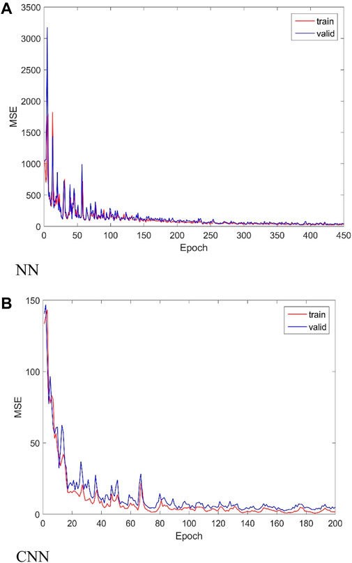
FIGURE 6. The MSE curves of the two methods. (A) NN. (B) CNN.

FIGURE 7

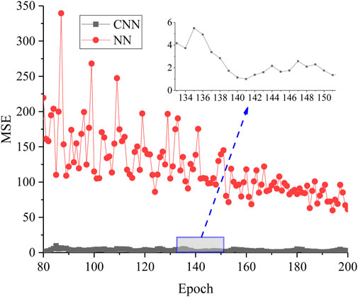
FIGURE 7. Comparison of the training loss curves between the two networks.

There were 387 samples in the test set. The predicted displacements are automatically generated by feeding these samples into the displacement estimation model generated by the above two methods. The predicted displacements based on the fully connected neural network are shown in Figure 8. From the figure, it can be seen that the predicted displacement curve based on the fully connected neural network method partially overlaps with the actual displacement curve, and the MSE of the test set is 29.489. It can be seen that the predicted displacements generated by the fully connected neural network have a good degree of overlap with the actual displacements.

FIGURE 8

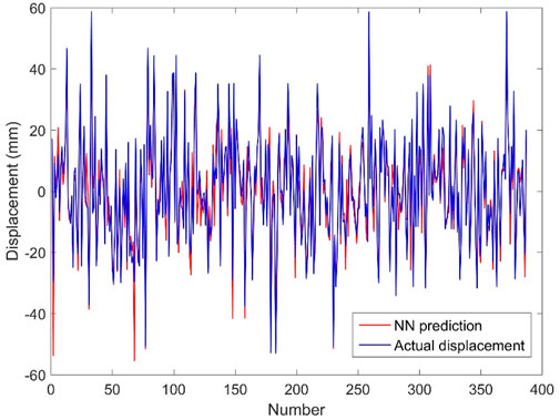
FIGURE 8. The predicted displacement based on NN.

The results of displacement prediction based on convolutional neural network are shown in Figure 9. It can be seen that the displacement curve predicted based on convolutional neural network has a great overlap with the actual displacement curve. The MSE of the test set is 3.096, which indicates that the CNN has high accuracy in estimating the dynamic displacement of the structure. For the same test set, the MSE of the convolutional neural network is much smaller than that of the fully connected neural network, and the number of training episodes of the convolutional neural network is also smaller than that of the fully connected neural network. Therefore, compared with the fully connected neural network, the proposed convolutional neural network performs better in displacement estimation with both higher estimation accuracy and higher modelling efficiency.

FIGURE 9

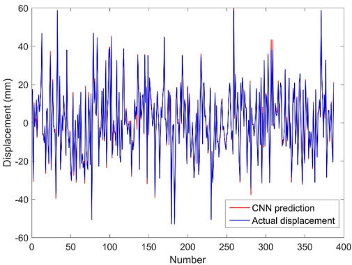
FIGURE 9. The predicted displacement based on CNN.

3.3 The effects of noise

Noise is inevitable in data acquisition systems. Meanwhile, disturbed by the external environment, there are often more noise signals and uncertainties in the sensor-based sensory data. In order to verify the noise resistance of the proposed convolutional neural network, four noise levels (i.e., noise-to-signal ratios of 10%, 20%, 30%, and 40%, respectively) are added to the acceleration signals to investigate the robustness of the CNN to noisy data. These data were directly fed into the trained dynamic displacement estimation model, which was trained and updated from noisy data samples. The dynamic displacement prediction results based on convolutional neural network are shown in Figure 10. It can be seen that the displacements predicted by the convolutional neural network still have good accuracy under the influence of noise. Since the effects of the four noise levels on the convolutional neural network are basically the same, only the predicted displacements based on the test set for two noise levels (10% and 40%) are shown in the figure. Four evaluation indicators (MSE, MAE, MAPE, and R²) based on the test set for each of the four noise levels are calculated in Table 3. These four-assessment metrics change very little as the noise-to-credit ratio continues to increase. Especially for R², its value is always 0.991. The results showed that the convolutional neural network is robust against noise. The noise of data acquisition has little effect on it because the convolutional and pooling layers in the convolutional neural network are similar to filters and are more powerful than normal filters.

FIGURE 10

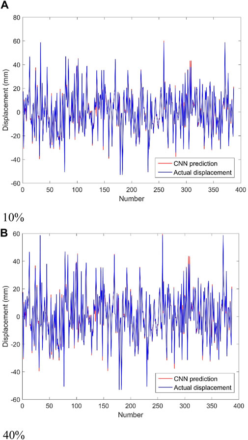
FIGURE 10. The predicted displacements based on test set with noise. (A) 10%. (B) 40%.

TABLE 3

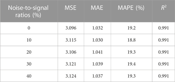
TABLE 3. Estimation error for test samples with varying degrees of noise.

4 Physical model test

4.1 Dataset generation

In Section 3, acceleration and displacement signals are generated by numerical simulation. The dataset is trained to estimate the dynamic displacements. However, the data generated by numerical simulation is idealized. The acceleration and displacement signals of the actual structure are acquired by sensors. The data collected by the sensors is incomplete and complex due to the noise and missing data characteristics of the sensors. Therefore, it is necessary to verify the effect of the proposed convolutional neural network on the actual structure. The design of the actual frame structure is shown in Figure 11. In the case where the real frame structure is subjected to transient excitation, the acceleration and displacement signals of the nodes are collected by piezoelectric accelerometers and laser displacement sensors. The piezoelectric accelerometers and laser displacement sensors are acquired at a frequency of 100 Hz. This real dynamic displacement estimation dataset is formed in the same way as in Section 3. The dataset contains a total of 2,333 samples, of which 1,600 samples are used as the training set, 400 samples are used as the validation set, and 333 samples are used as the test set.

FIGURE 11

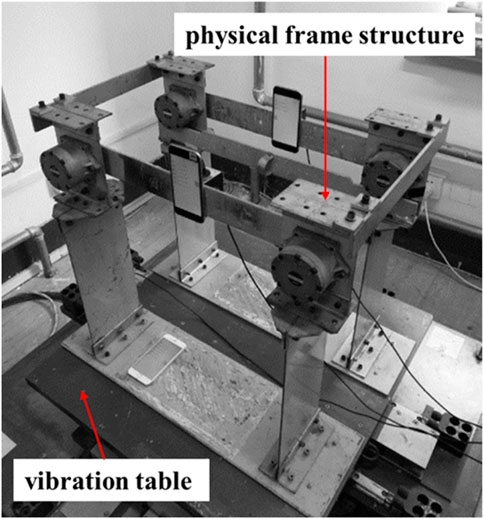
FIGURE 11. Physical frame structure.

4.2 Estimation result

The training set is fed into the proposed convolutional neural network. The MSE curve is shown in Figure 12. It can be seen that the MSE curve remains almost constant when the epoch is 250. This indicates that the model has basically reached the convergence state. The MSE based on the training set is 5.097 and the MSE based on the validation set is 10.770. The MSE value can satisfy the need of engineering design.

FIGURE 12

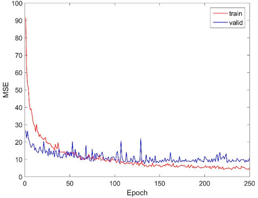
FIGURE 12. The MSE curves.

The test set contains 333 samples and the test set is fed into the dynamic displacement estimation model. The predicted and actual displacements are shown in Figure 13. It can be seen that the predicted displacement curves are in high agreement with the actual displacement curves. The MSE based on the test set is 6.150. The results show that the displacement estimation method based on convolutional neural network can accurately estimate the displacement signal using the acceleration signal.

FIGURE 13

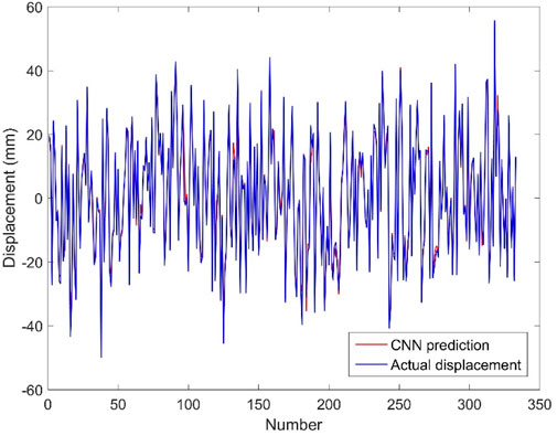
FIGURE 13. The predicted displacements and actual displacements.

4.3 Visualization of the output

A neural network is similar to a black box. It is difficult to understand and does not give direct visualization of the output. Data processing in neural networks is invisible. Convolutional neural network is one of the neural networks which also has this characteristic. Therefore, in order to have a clearer understanding of how convolutional neural networks process data, we have visualized the output of the hidden layer of the convolutional neural network. The proposed convolutional neural network consists of an input layer, four convolutional layers, a pooling layer, a flattening layer and an output (dense) layer. In convolutional neural network, convolutional and pooling layers are the core components.

In this section, the output of the convolutional layer and the pooling layer is visualized. The first sample data in the test set is shown in Figure 14A, and the curve fluctuates between 150 and 1000 mm/s². The input data is passed to the first convolutional layer. The first convolutional layer has 6 convolutional kernels. Each convolution kernel processes the input data to produce a 46 × 1 vector. Therefore, there are 6 vectors (46 × 1). One of the vectors is shown in Figure 14B, where the curve fluctuates between 50 and 300. The second convolutional layer has 12 convolutional kernels, and there are 12 vectors (42 × 1). One of the vectors is shown in Figure 14C, and the curve fluctuates between 0 and 100. The third convolutional layer has 64 convolutional kernels and a total of 64 vectors (38 × 1). One of the vectors is shown in Figure 14D, and the curve fluctuates between 3 and 16. The fourth convolutional layer has 128 convolutional kernels with 128 vectors (34 × 1). One of the vectors is shown in Figure 14E, and the curve fluctuates between 0 and 2. As the data is processed through the convolutional layers, the value of each data becomes smaller. The pooling layer has 128 convolutional kernels and a total of 128 vectors (17 × 1). One of the vectors is shown in Figure 14F, where the curve fluctuates between 0 and 2. It can be seen that the pooling layer does not change the value of the data, but reduces the amount of data. The data curve becomes smoother after the data is processed by the pooling layer. The convolutional and pooling layers can also act as filters, so the convolutional neural network has strong noise immunity. Although the size of the output vector of the hidden layer is decreasing, the overall shape of the original data is still well preserved.

FIGURE 14

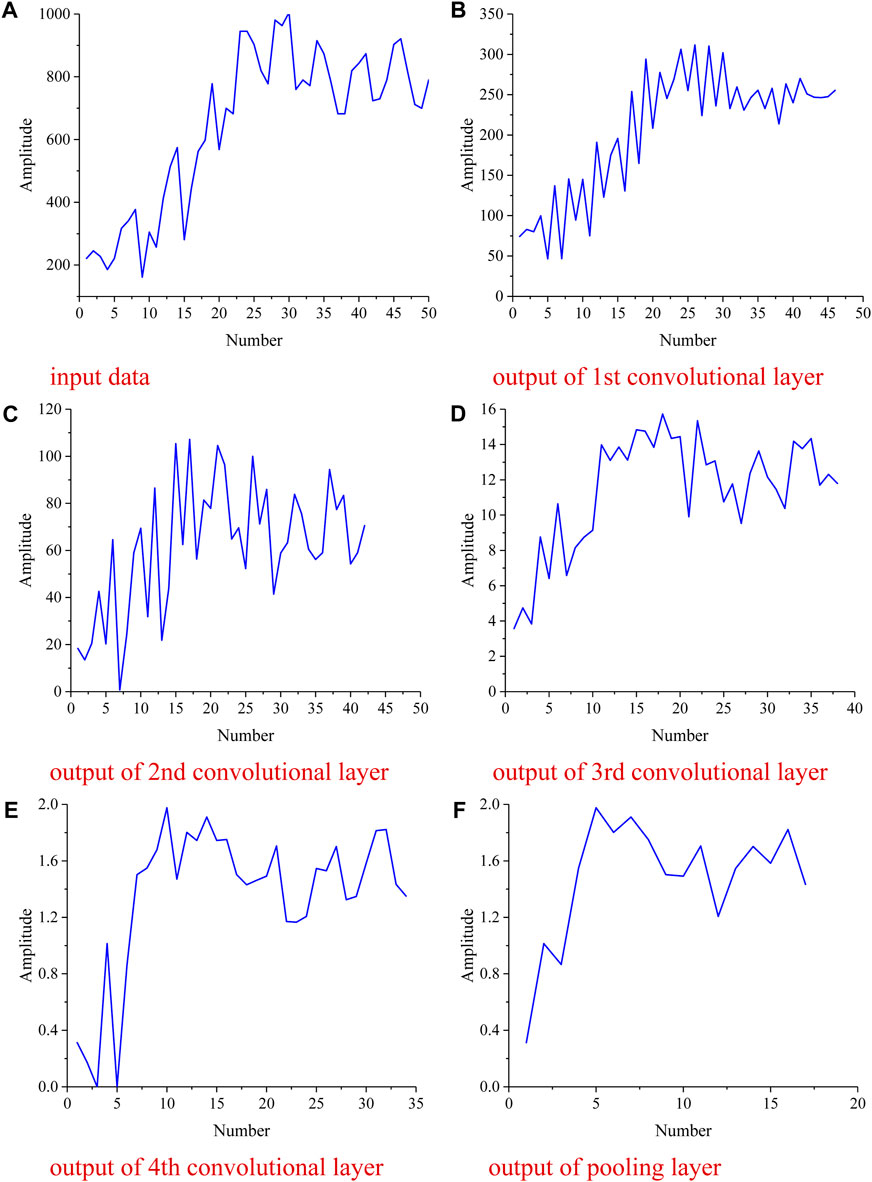
FIGURE 14. The output of hidden layers. (A) input data. (B) output of 1st convolutional layer. (C) output of 2nd convolutional layer. (D) output of 3rd convolutional layer. (E) output of 4th convolutional layer. (F) output of pooling layer.

The output of the pooling layer is a multidimensional vector. The Flatten layer then converts the multidimensional vectors into one-dimensional vectors. The Flatten layer rearranges the data into a one-dimensional form, preserving the feature order of the multidimensional vectors. This allows the subsequent Fully Connected layer to learn based on the overall features of the input and to model the relationships between the features. The one-dimensional vectors are fed into the fully connected (dense) layer. Finally, an estimate of the dynamic displacement is output. Table 4 shows the predicted and actual values of the first 10 samples in the test set. It can be seen that only the sixth and ninth samples have an error greater than 10%, while the other samples have an error between 0.15% and 9.30%. The average error is 6.69%, so the proposed method can meet the engineering needs.

TABLE 4

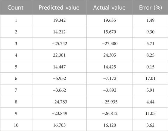
TABLE 4. The predicted error of test set.

5 Discussion

In this paper, a 1D convolutional neural network is used for data-driven modelling of the complex relationship between acceleration signals and dynamic displacements. The dynamic displacement estimation method based on convolutional neural network is verified by numerical simulation to be superior to the method based on fully connected neural network in terms of accuracy, stability and convergence efficiency. Noise is added to the test set and these data are directly fed into the dynamic displacement estimation model which is trained from noise-free data samples. It is worth noting that the displacements estimated by the convolutional neural network model still have good accuracy under the influence of noise. Subsequently, a real frame structure is used to verify the feasibility of the proposed method in real engineering applications. Although the root-mean-square error of the predicted displacements of the real structure is larger than the root-mean-square error of the predicted displacements of the finite element model, the predicted displacements of the real structure satisfy the engineering needs. This is mainly due to the fact that the sensors are affected by many factors when sensing the dynamic characteristics of the structure, and the collected signals contain more noise and uncertainty. The results of the output visualization of the convolutional neural network show that the convolution operation not only reduces the amount of data, but also reduces the data values. In addition, the convolutional and pooling layers act as filters, which results in a convolutional neural network with strong noise immunity.

6 Conclusion

In this paper, a dynamic displacement estimation method based on convolutional neural network and acceleration is proposed. The acceleration and displacement signals are trained to generate an estimation model. The acceleration data is input into this estimation model, and the displacement estimate can be output automatically. Numerical simulations and physical model tests verify the feasibility and stability of the method. Some important results are obtained: the 1D convolutional neural network can accurately model the complex relationship between acceleration timing signals and displacement signals; the convergence efficiency of the convolutional neural network is much greater than that of a typical neural network when modelling the complex relationship using the convolutional neural network. The updating efficiency of the former is 2.25 times that of the latter; due to the existence of the convolution kernel in the convolutional neural network, it can filter the data and has a strong anti-noise ability; in this paper, the visualization part at the end fully reflects the filtering effect of the convolution kernel on the noise. The proposed method can easily and quickly estimate the dynamic displacement of structures using acceleration information. It also still shows good results in noisy environments. However, the proposed method is affected by the accuracy of the acceleration signal. To further improve the accuracy of displacement estimation, multi-sensor fusion such as accelerometers and strain gauges can be considered. In addition, deep learning architectures based on multi-sensor fusion need to be further explored.

Data availability statement

The raw data supporting the conclusion of this article will be made available by the authors, without undue reservation.

Author contributions

XZ: Data curation, Formal Analysis, Methodology, Validation, Visualization, Writing–original draft. YH: Conceptualization, Resources, Supervision, Writing–review and editing.

Funding

The authors declare that no financial support was received for the research, authorship, and/or publication of this article.

Conflict of interest

The authors declare that the research was conducted in the absence of any commercial or financial relationships that could be construed as a potential conflict of interest.

Publisher’s note

All claims expressed in this article are solely those of the authors and do not necessarily represent those of their affiliated organizations, or those of the publisher, the editors and the reviewers. Any product that may be evaluated in this article, or claim that may be made by its manufacturer, is not guaranteed or endorsed by the publisher.

References

1. Park J-W, Lee JJ, Jung HJ, Myung H. Vision-based displacement measurement method for high-rise building structures using partitioning approach. Ndt E Int (2010) 43(7):642–7. doi:10.1016/j.ndteint.2010.06.009

CrossRef Full Text | Google Scholar

2. Zhang Y, Wang T, Yuen K-V. Construction site information decentralized management using blockchain and smart contracts. Computer-Aided Civil Infrastructure Eng (2022) 37(11):1450–67. doi:10.1111/mice.12804

CrossRef Full Text | Google Scholar

3. Chan THT, Yu L, Tam H, Ni Y, Liu S, Chung W, et al. Fiber Bragg grating sensors for structural health monitoring of Tsing Ma bridge: background and experimental observation. Eng structures (2006) 28(5):648–59. doi:10.1016/j.engstruct.2005.09.018

CrossRef Full Text | Google Scholar

4. Zhang Y, Yuen K-V. Review of artificial intelligence-based bridge damage detection. Adv Mech Eng (2022) 14(9):168781322211227. doi:10.1177/16878132221122770

CrossRef Full Text | Google Scholar

5. He Y, Zhou Q, Xu F, Sheng X, He Y, Han J. An investigation into the effect of rubber design parameters of a resilient wheel on wheel-rail noise. Appl Acoust (2023) 205:109259. doi:10.1016/j.apacoust.2023.109259

CrossRef Full Text | Google Scholar

6. He Y, Zhang Y, Yao Y, He Y, Sheng X. Review on the prediction and control of structural vibration and noise in buildings caused by rail transit. Buildings (2023) 13:2310. doi:10.3390/buildings13092310

CrossRef Full Text | Google Scholar

7. Lynch JP, Loh KJ. A summary review of wireless sensors and sensor networks for structural health monitoring. Shock Vibration Dig (2006) 38(2):91–128. doi:10.1177/0583102406061499

CrossRef Full Text | Google Scholar

8. Giurgiutiu V, Zagrai A, Bao JJ. Piezoelectric wafer embedded active sensors for aging aircraft structural health monitoring. Struct Health Monit (2002) 1(1):41–61. doi:10.1177/147592170200100104

CrossRef Full Text | Google Scholar

9. Farrar CR, Keith W. An introduction to structural health monitoring. Phil Trans R Soc A: Math Phys Eng Sci (2006) 365(1851):303–15. doi:10.1098/rsta.2006.1928

PubMed Abstract | CrossRef Full Text | Google Scholar

10. Park G, Rosing T, Todd MD, Farrar CR, Hodgkiss W. Energy harvesting for structural health monitoring sensor networks. J Infrastructure Syst (2008) 14(1):64–79. doi:10.1061/(asce)1076-0342(2008)14:1(64)

CrossRef Full Text | Google Scholar

11. Amann M-C, Bosch T. M., Lescure M., Myllylae R. A., Rioux M., et al. Laser ranging: a critical review of unusual techniques for distance measurement. Opt Eng (2001) 40(1):10–20. doi:10.1117/1.1330700

CrossRef Full Text | Google Scholar

12. Bitou Y, Schibli TR, Minoshima K. Accurate wide-range displacement measurement using tunable diode laser and optical frequency comb generator. Opt express (2006) 14(2):644–54. doi:10.1364/opex.14.000644

PubMed Abstract | CrossRef Full Text | Google Scholar

13. Lee JJ, Fukuda Y, Shinozuka M, Cho S, Yun CB. Development and application of a vision-based displacement measurement system for structural health monitoring of civil structures. Smart Structures Syst (2007) 3(3):373–84. doi:10.12989/sss.2007.3.3.373

CrossRef Full Text | Google Scholar

14. Feng D, Feng M, Ozer E, Fukuda Y. A vision-based sensor for noncontact structural displacement measurement. Sensors (2015) 15(7):16557–75. doi:10.3390/s150716557

PubMed Abstract | CrossRef Full Text | Google Scholar

15. Rice JA, Li C, Gu C, Hernandez JC. A wireless multifunctional radar-based displacement sensor for structural health monitoring. In: Proceedings of the Sensors and Smart Structures Technologies for Civil, Mechanical, and Aerospace Systems; April 2011; San Diego, California, USA (2011). doi:10.1117/12.879243

CrossRef Full Text | Google Scholar

16. Yi TH, Li HN, Gu M. Recent research and applications of GPS-based monitoring technology for high-rise structures. Struct Control Health Monit (2013) 20(5):649–70. doi:10.1002/stc.1501

CrossRef Full Text | Google Scholar

17. Sabatini AM, Ligorio G, Mannini A. Fourier-based integration of quasi-periodic gait accelerations for drift-free displacement estimation using inertial sensors. Biomed Eng Online (2015) 14(1):106. doi:10.1186/s12938-015-0103-8

PubMed Abstract | CrossRef Full Text | Google Scholar

18. Park K-T, Kim SH, Park HS, Lee KW. The determination of bridge displacement using measured acceleration. Eng Structures (2005) 27(3):371–8. doi:10.1016/j.engstruct.2004.10.013

CrossRef Full Text | Google Scholar

19. Roberts GW, Meng X, Dodson AH. Integrating a global positioning system and accelerometers to monitor the deflection of bridges. J Surv Eng (2004) 130(2):65–72. doi:10.1061/(asce)0733-9453(2004)130:2(65)

CrossRef Full Text | Google Scholar

20. Gindy M, Vaccaro R, Nassif H, Velde J. A state-space approach for deriving bridge displacement from acceleration. Computer-Aided Civil Infrastructure Eng (2008) 23(4):281–90. doi:10.1111/j.1467-8667.2007.00536.x

CrossRef Full Text | Google Scholar

21. Rui Z, Min F, Dou Y, Ye B. Switching mechanism and hardware experiment of a non-smooth Rayleigh-Duffing system. Chin J Phys (2023) 82:134–48. doi:10.1016/j.cjph.2023.02.001

CrossRef Full Text | Google Scholar

22. Yao W, Wang C, Sun Y, Gong S, Lin H. Event-triggered control for robust exponential synchronization of inertial memristive neural networks under parameter disturbance. Neural Networks (2023) 164:67–80. doi:10.1016/j.neunet.2023.04.024

PubMed Abstract | CrossRef Full Text | Google Scholar

23. Yao W, Wang C, Sun Y, Zhou C. Robust multimode function synchronization of memristive neural networks with parameter perturbations and time-varying delays. IEEE Trans Syst Man, Cybernetics: Syst (2020) 52(1):260–74. doi:10.1109/tsmc.2020.2997930

CrossRef Full Text | Google Scholar

24. Yao W, Gao K, Zhang Z, Cui L, Zhang J. An image encryption algorithm based on a 3D chaotic Hopfield neural network and random row–column permutation. Front Phys (2023) 11:1162887. doi:10.3389/fphy.2023.1162887

CrossRef Full Text | Google Scholar

25. Krizhevsky A, Sutskever I, Hinton GE. Imagenet classification with deep convolutional neural networks. Adv Neural Inf Process Syst (2012).

Google Scholar

26. Simonyan K, Zisserman A. Very deep convolutional networks for large-scale image recognition (2014). Availab;e at: https://arxiv.org/abs/1409.1556.

Google Scholar

27. Karpathy A, Toderici G, Shetty S, Leung T, Sukthankar R, Fei-Fei L, et al. Large-scale video classification with convolutional neural networks. In: Proceedings of the IEEE conference on Computer Vision and Pattern Recognition; June 2014; Columbus, OH, USA (2014).

CrossRef Full Text | Google Scholar

28. He K, Zhang X, Ren S, Sun J, et al. Deep residual learning for image recognition. In: Proceedings of the IEEE conference on computer vision and pattern recognition; June 2016; Las Vegas, NV, USA (2016).

CrossRef Full Text | Google Scholar

29. Esteva A, Kuprel B, Novoa RA, Ko J, Swetter SM, Blau HM, et al. Dermatologist-level classification of skin cancer with deep neural networks. Nature (2017) 542(7639):115–8. doi:10.1038/nature21056

PubMed Abstract | CrossRef Full Text | Google Scholar

30. Moeskops P, Viergever MA, Mendrik AM, de Vries LS, Benders MJNL, Isgum I. Automatic segmentation of MR brain images with a convolutional neural network. IEEE Trans Med Imaging (2016) 35(5):1252–61. doi:10.1109/tmi.2016.2548501

PubMed Abstract | CrossRef Full Text | Google Scholar

31. CireşAn D, Meier U, Masci J, Schmidhuber J. Multi-column deep neural network for traffic sign classification. Neural networks (2012) 32:333–8. doi:10.1016/j.neunet.2012.02.023

PubMed Abstract | CrossRef Full Text | Google Scholar

32. Jin J, Fu K, Zhang C. Traffic sign recognition with hinge loss trained convolutional neural networks. IEEE Trans Intell Transportation Syst (2014) 15(5):1991–2000. doi:10.1109/tits.2014.2308281

CrossRef Full Text | Google Scholar

33. Cha Y-J, Choi W, Büyüköztürk O. Deep learning-based crack damage detection using convolutional neural networks. Computer-Aided Civil Infrastructure Eng (2017) 32(5):361–78. doi:10.1111/mice.12263

CrossRef Full Text | Google Scholar

34. Zhang Y, Yuen K-V. Crack detection using fusion features-based broad learning system and image processing. Computer-Aided Civil Infrastructure Eng (2021) 36(12):1568–84. doi:10.1111/mice.12753

CrossRef Full Text | Google Scholar

35. Ge Y, Zhu F, Chen D, Zhao R, Wang X, Li H. Structured domain adaptation with online relation regularization for unsupervised person re-id. IEEE Trans Neural Networks Learn Syst (2022) 1–14. doi:10.1109/tnnls.2022.3173489

CrossRef Full Text | Google Scholar

36. Du F, Wu S, Xing S, Xu C, Su Z. Temperature compensation to guided wave-based monitoring of bolt loosening using an attention-based multi-task network. Struct Health Monit (2023) 22(3):1893–910. doi:10.1177/14759217221113443

CrossRef Full Text | Google Scholar

37. Zhang Y, Yuen K-V. Bolt damage identification based on orientation-aware center point estimation network. Struct Health Monit (2022) 21(2):438–50. doi:10.1177/14759217211004243

CrossRef Full Text | Google Scholar

38. Li L, Sun HX, Zhang Y, Yu B. Surface cracking and fractal characteristics of bending fractured polypropylene fiber-reinforced geopolymer mortar. Fractal and Fractional (2021) 5(4):142. doi:10.3390/fractalfract5040142

CrossRef Full Text | Google Scholar

39. Li L, Zhang Y, Shi Y, Xue Z, Cao M. Surface cracking and fractal characteristics of cement paste after exposure to high temperatures. Fractal and Fractional (2022) 6(9):465. doi:10.3390/fractalfract6090465

CrossRef Full Text | Google Scholar

40. Zhang Y, Yuen KV. Time-frequency fusion features-based incremental network for smartphone measured structural seismic response classification. Eng Structures (2023) 278:115575. doi:10.1016/j.engstruct.2022.115575

CrossRef Full Text | Google Scholar

41. Zhang Y, Yuen KV, Mousavi M, Gandomi AH. Timber damage identification using dynamic broad network and ultrasonic signals. Eng Structures (2022) 263:114418. doi:10.1016/j.engstruct.2022.114418

CrossRef Full Text | Google Scholar

42. Malek S, Melgani F, Bazi Y. One-dimensional convolutional neural networks for spectroscopic signal regression. J Chemometrics (2018) 32(5):e2977. doi:10.1002/cem.2977

CrossRef Full Text | Google Scholar

43. Hasegawa C, Iyatomi H. One-dimensional convolutional neural networks for Android malware detection. In: Proceedings of the 2018 IEEE 14th International Colloquium on Signal Processing & Its Applications (CSPA); March 2018; Penang, Malaysia. IEEE (2018).

CrossRef Full Text | Google Scholar

44. Shrestha A, Mahmood A. Review of deep learning algorithms and architectures. IEEE access (2019) 7:53040–53065. doi:10.1109/ACCESS.2019.2912200

CrossRef Full Text | Google Scholar

45. Glorot X, Antoine B, Bengio Y. Deep sparse rectifier neural networks. In: Proceedings of the Proceedings of the 14th International Conference on Artificial Intelligence and Statistics (AISTATS); April 2011; Fort Lauderdale, FL, USA (2011).

Google Scholar

46. Gu J, Wang Z, Kuen J, Ma L, Shahroudy A, Shuai B, et al. Recent advances in convolutional neural networks. Pattern recognition (2018) 77:354–77. doi:10.1016/j.patcog.2017.10.013

CrossRef Full Text | Google Scholar

47. Kim P, Kim P. Convolutional neural network. In: MATLAB deep learning: with machine learning, neural networks and artificial intelligence. Berlin, Germany: Springer (2017). p. 121–47.

CrossRef Full Text | Google Scholar