Numerical treatment of a magnetized electron fluid model in a 3D simulator of plasma thruster plumes

Simulations of energetic plumes from plasma thrusters are of great interest for estimating performances and interactions with the spacecraft. Both in fully fluid and hybrid (particle/fluid) models, the electron population is described by a set of fluid equations whose resolution by different numerical schemes can be strongly affected by convergence and accuracy issues. The case of magnetized plumes is more critical. Here, the numerical discretization of the electron fluid model of a 3D hybrid simulator of plasma plumes was upgraded from a finite-differences (FD) formulation in a collocated grid to a finite-volumes (FV) approach in a staggered grid. Both approaches make use of structured meshes of different resolutions and are compared in two scenarios of interest: 1) an unmagnetized plasma plume around a spacecraft and 2) a magnetized plume expansion in free space. In both physical scenarios, the FD scheme exhibits a global continuity error related to truncation errors that can be reduced only by refining the mesh. The origin of this error is further investigated and explained here. The FV scheme instead can save much computational time using coarser meshes since it is unaffected by these errors due to the conservativeness of its formulation. The physical advantage of the FV scheme over the FD approach is more evident for magnetized plumes with high Hall parameters since it allows us to reach higher anisotropy conditions, here assessed in order to gain insights into the plume magnetization effects, finding that the already foreseen saturation of circulating electric current occurs for Hall parameters of several hundreds.

1 Introduction

Electric thrusters for space propulsion [1] eject a plasma plume, which is made of hypersonic ions moving at speeds of tens of km/s and a cloud of confined electrons that drifts with a comparable velocity to guarantee current ambipolarity. The peak electron temperature at the thruster exit is typically in the range of 5–50 eV, depending on the thruster technology [2]. These plasma plumes can be either unmagnetized, as in the case of an ion thruster (IT), or magnetized, meaning that electrons are bound to the lines of an externally generated magnetic field, as in Hall-effect thrusters (HETs) or in electrodeless plasma thrusters (EPTs), featuring a divergent magnetic nozzle (MN) for plasma plume expansion and acceleration [3]. Ions, on the other hand, are nearly unmagnetized in these thrusters, with a Larmor radius exceeding the characteristic plume size by several orders of magnitudes. When operating in low Earth orbits, all plasma thruster plumes are further affected by the presence of the geomagnetic field of a magnitude of approximately 0.5 G, which can induce non-trivial three-dimensional electron and electric current structures [4–6], yielding to significant plasma plume deformation farther downstream.

In the context of plasma plumes for space propulsion, simulations are extremely important as they enable the study of two fundamental phenomena: 1) spacecraft–plume interaction, which is paramount for a correct installation of electric thrusters onboard the satellite platform, minimizing their negative impact on sensitive surfaces, such as optical sensors or solar arrays [7], and 2) facility effect estimation, required to extrapolate the performance of a thruster tested inside a vacuum chamber to real in-space operations. Numerical models for magnetized plasma plume expansions include kinetic approaches, which can be split into methods solving a simplified Boltzmann’s equation for the ion and electron distribution functions [8] and full particle-in-cell (PIC) techniques [9, 10], featuring ion and electron macro-particles, and treating collisions through Monte Carlo techniques. These approaches are extremely expensive from a computational point of view, especially when it comes to plume expansions [11], for which other approaches are more computationally efficient. In particular, hybrid models [11–15], in which electrons are assumed as a magnetized or unmagnetized fluid while ions are followed as PIC macro-particles, and fully fluid models [5, 16, 17], where both ions and electrons are treated as one or more fluids, are computationally much more affordable. In these cases, electrons are described by a set of differential equations for continuity, momentum, and energy [18, 19]. A magnetic field introduces strong anisotropy in electron mobility, and the solution of these equations is strongly affected by convergence and accuracy issues, which depend on the numerical scheme adopted. This greatly limits the application of magnetized electron fluid models to 2D scenarios, as shown in [17], with only a few examples of 3D magnetized electron models existing in the literature [4, 6, 15, 20, 21].

Electron fluid models can employ different discretization schemes for a set of differential equations. A common classification features the following [22, 23]: 1) finite differences (FD) schemes, 2) finite elements (FE) methods, 3) finite volumes (FV) methods, and 4) spectral methods [24]. Narrowing the field, gradient terms can be discretized with an FD approach, while, for conservation equations, FV, FE, or FD discretization can be adopted. Although FE methods use variational techniques to minimize an error function, FV methods are normally the most conservative by definition since the conservation equations are expressed and discretized in their integral form on a control volume, and the flux entering a given volume is set equal to that leaving the adjacent volume. This allows us to represent the mass and energy balances consistently, while momentum and heat flux equations can still be discretized with an FD approach. On the other hand, if a conventional FD approach is also used for the discretization of continuity equations and of their corresponding right-hand sides, global continuity errors can arise, coming from the derivative truncation error at every order of accuracy. Although there exist flux-conserving FD approaches, they employ high-order reconstruction schemes to guarantee conservativeness, thus being more computationally burdening. This focus on FD and FV methods comes from the fact that they share many similarities and can lead to the same discretization in some cases [25], eventually causing confusion when it comes to the choice of the scheme.

EP2PLUS is a 3D PIC-fluid code for magnetized and unmagnetized plumes [11], where 1) electrons are modeled as a magnetized fluid subject to both continuity and momentum balance equations and a polytropic pressure closure; 2) ions are followed as macro-particles of a PIC submodel, which move according to the local electric and magnetic fields, and are subject to discrete collisional events, through standard Monte Carlo collision (MCC) techniques. The PIC and the electron fluid meshes coincide and are of structured Cartesian type, non-uniform in space, in general. In this work, EP2PLUS, which originally solved the electron fluid equations with an FD formulation [4, 11], is upgraded to employ an FV conservative method on a staggered grid for the electron continuity equation. The new FV approach is benchmarked against the previous FD approach in two 3D physical scenarios of interest: 1) an unmagnetized plasma–spacecraft interaction scenario, introduced in [11], and 2) a magnetized plasma plume expansion under the effect of a geomagnetic field, first studied with an FD approach in [4]. Both scenarios feature a structured mesh, although of different types. This paper then aims to compare and benchmark the two particular formulations of FD and FV methods first in terms of the conservativeness and quality of the obtained solution for a varying mesh resolution; second, for magnetized plumes only, in terms of the maximum allowed Hall parameter for a reasonable solution quality.

The rest of the paper is structured as follows: Section 2 describes the hybrid PIC-fluid model considered, with emphasis on the latter; Section 3 focuses on the numerical schemes for the resolution of electron fluid equations; Section 4 reports the settings and simulation results for the chosen unmagnetized benchmark scenario, while Section 5 reports the settings and simulation results for the magnetized scenario, in which the new FV scheme enables to extend a previous study [4] on the effects of the maximum simulated transport anisotropy. Conclusions and future work are summarized in Section 6.

2 The plasma plume model

The plasma plume model assumes both ions and neutrals as macro-particles of a PIC submodel and electrons as a magnetized fluid. The PIC and electron submodels are described in the following paragraphs, with a special emphasis on the latter. In addition to PIC and electron fluid submodels, both a plasma sheath and circuit solver models are used to obtain the appropriate boundary conditions (BCs) for the electron fluid (in terms of electric current reaching the surface of simulated objects). This latter feature is relevant mainly for the simulations of the spacecraft–plasma interaction; details can be found in [11].

2.1 The particle-in-cell submodel

A detailed description of the PIC submodel used for the heavy species can be found in [11, 26]. This advances both ion and neutral macro-particles with the same PIC time step and includes a series of algorithms: 1) particle injection from an upstream boundary, which typically coincides with the thruster exhaust section; 2) particle movement, according to Newton’s equation and the local electric and magnetic fields E and B; 3) particle collisions, including ionization and charge-exchange reactions (CEX) with MCC techniques; 4) particle interaction with the material walls of the spacecraft (S/C), if any, including the computation of the ion current density to the material cell faces, ion recombination into neutrals, and neutral reflection; and 5) particle weighting to the nodes of the PIC mesh to obtain plasma bulk properties, such as the number density and the particle fluxes of each species.

2.2 The electron submodel

For a quasi-stationary (∂/∂t = 0) and inertialess electron fluid, the electron momentum equation reads

$0=-\nabla p_{\text{e}}-e{n}_{\text{e}}\left(-\nabla \varphi +{\mathit{u}}_{\text{e}}\times \mathit{B}\right)-{\displaystyle \sum _s}{\nu }_{\text{e}s}{m}_{\text{e}}{n}_{\text{e}}\left({\mathit{u}}_{\text{e}}-{\mathit{u}}_s\right),(1)$

where n_e represents the electron number density, m_e represents the electron mass, u_e represents the electron fluid velocity, ϕ represents the electric potential, B represents the externally applied magnetic field, index s extends to all heavy populations (neutrals, singly or doubly charged ions, …), and ν_es represents the momentum transfer collision frequency of the electrons with the generic s^th particle population, which features a fluid velocity u_s. Additionally, Eq. 1 assumes isotropic electrons with a scalar pressure p_e ≡ n_eT_e, with T_e in appropriate energy units.

For the purposes of this work, the electron fluid model is closed, assuming a polytropic equation of state $p_{\text{e}}\propto n_{\text{e}}^{\gamma }$, with γ ≥1 as a constant coefficient. Then, it is possible to define a barotropy function [11]

$h_{\text{e}}\left(n_{\text{e}}\right)=\left\{\begin{array}{cc}{T}_{\text{e0}}\ln \left(\frac{n_{\text{e}}}{n_{\text{e0}}}\right),\hfill & \gamma =1,\hfill \\ -\frac{\gamma T_{\text{e0}}}{\gamma -1}\left[1-{\left(\frac{n_{\text{e}}}{n_{\text{e0}}}\right)}^{\gamma -1}\right],\hfill & \gamma >1,\hfill \end{array}\right.(2)$

satisfying ∇h_e = ∇p_e/n_e and with T_e0 and n_e0 reference values at the point where h_e = 0. Furthermore, it is convenient for the numerical schemes to define the thermalized potential [4]

$\mathrm{\Phi }=\varphi -h_{\text{e}}/e.(3)$

We observe that if Φ = 0 everywhere, ϕ(n_e) satisfies the Boltzmann’s polytropic relation.

We let j_e = −en_eu_e and j_i = ∑_seZ_sn_su_s be the electron and total ion current density (with Z_s and n_s as the charge number and the number density of the generic s^th particle population, respectively); ν_e = ∑_sν_es represents the total electron momentum transfer collision frequency; ${\mathit{j}}_{\text{c}}=(e{n}_{\text{e}}/{\nu }_{\text{e}}){\sum }_{s=1}^L{\nu }_{\text{e}s}{\mathit{u}}_s$ represents an effective current density grouping collisional effects from heavy species [4]; σ_e = e²n_e/(m_eν_e) represents the electron scalar conductivity; χ = ω_ce/ν_e represents the Hall parameter, with ω_ce = eB/m_e being the electron gyrofrequency; and ${\mathbf{1}}_{\text{b}}=\left[b_1,b_2,b_3\right]$ the unit vector locally aligned with the applied magnetic field so that B = B1_b. Applying all these definitions and solving Eq. 1 for the total electric current density, j = j_e + j_i, yields the generalized Ohm’s law

$\mathit{j}=-\mathcal{K}\cdot \left({\sigma }_{\text{e}}\nabla \mathrm{\Phi }+{\mathit{j}}_{\text{c}}\right)+{\mathit{j}}_{\text{i}},(4)$

where

$\mathcal{K}={\left[\begin{array}{ccc}\hfill 1\hfill & \hfill \chi b_3\hfill & \hfill -\chi b_2\hfill \\ \hfill -\chi b_3\hfill & \hfill 1\hfill & \hfill \chi b_1\hfill \\ \hfill \chi b_2\hfill & \hfill -\chi b_1\hfill & \hfill 1\hfill \end{array}\right]}^{-1}(5)$

is the normalized conductivity tensor, for which ${\mathcal{K}}^{-1}\mathit{j}=\mathit{j}+\chi \left(\mathit{j}\times {\mathbf{1}}_{\text{b}}\right)$.

The additional scalar equation to solve for the four scalar unknowns (Φ and j) is the electric current continuity

$\nabla \cdot \mathit{j}=0.(6)$

The system of Eqs 4, 6 is solved by applying boundary conditions either on Φ (i.e., Dirichlet condition) or, more commonly, on the normal component of the local electric current density, j_n ≡j ⋅1_n (i.e., a Neumann condition), with 1_n being the normal unit vector at the boundaries, directed toward the plasma. BCs are typically an issue in plume models; the effects of different formulations have been investigated in [4, 27].

Once the Φ value is obtained, the electric potential is retrieved from Eq. 3. Although the barotropic function h_e (n_e) is updated at each PIC time step as it depends only on n_e, the thermalized potential Φ is updated with a lower cadence. This permits us to save computational time and has no impact on the final solution, as long as we are primarily interested in stationary plasma plumes. In low-density non-neutral sub-regions of the plume, a non-linear Poisson’s equation is solved, in order to retrieve the non-neutral plasma density and electric potential:

${\nabla }^2\varphi =\frac{e}{{\epsilon }_0}\left(n_{\text{e}}\left(\varphi \right)-{\displaystyle \sum _s}{Z}_s{n}_s\right),(7)$

where n_e(ϕ) is given by Eq. 3 (with the use of Eq. 2). The computational domain is indeed split into quasi-neutral, non-neutral, and transition regions, according to the physical criteria described in [11].

3 Numerical approaches for electron fluid equations

3.1 The old finite difference solution scheme

Substituting Eq. 4 into Eq. 6, an elliptic equation for Φ is obtained:

$\mathcal{K}:\nabla \nabla \mathrm{\Phi }+\nabla \mathrm{\Phi }\cdot \left(\nabla \cdot \mathcal{K}\right)+\mathcal{K}\cdot \nabla \mathrm{\Phi }\cdot \nabla \ln \left({\sigma }_{\text{e}}\right)=\frac{\nabla \cdot \left({\mathit{j}}_{\text{i}}-\mathcal{K}\cdot {\mathit{j}}_{\text{c}}\right)}{{\sigma }_{\text{e}}},(8)$

where ∇∇Φ represents the Hessian tensor of the thermalized potential, the symbol “:” means a contracted product, and $\nabla \cdot \mathcal{K}$ represents the divergence of the conductivity tensor. Each term of Eq. 8 can be discretized using FD schemes of 2nd-order accuracy on a structured mesh, given as follows.

A generic 3D physical domain in (x, y, and z) is represented by a parallelepiped in the computational domain, with each mesh node being identified by three integer computational coordinates (ξ, η, and ζ) along the three structured mesh directions.

If the number of nodes along each direction is N_ξ, N_η, and N_ζ, such computational coordinates can vary within the ranges $\left[1,N_{\xi }\right]$, $\left[1,N_{\eta }\right]$, and $\left[1,N_{\zeta }\right]$. Generalized difference schemes on a non-rectangular, non-uniform physical mesh require the computation of the inverse Jacobian matrix, given as

${\left({\mathcal{J}}^{-1}\right)}_{ij}=\frac{\partial x_i}{\partial {\xi }_j},(9)$

where (x₁, x₂, x₃) ≡ (x, y, z) and (ξ₁, ξ₂, ξ₃) ≡ (ξ, η, ζ). Each Jacobian term is evaluated with an FD scheme of 2nd-order accuracy, applied to the nodes physical coordinates (x, y, and z). In particular, centered schemes with two nodes are applied to inner nodes, and forward/backward schemes (involving three nodes) are applied to the boundaries, along each direction. The direct transformation matrix $\mathcal{J}$ then appears in generalized difference schemes for the derivatives of Φ, given as

$\frac{\partial \mathrm{\Phi }}{\partial x_i}=\frac{\partial \mathrm{\Phi }}{\partial {\xi }_j}\frac{\partial {\xi }_j}{\partial x_i}=\frac{\partial \mathrm{\Phi }}{\partial {\xi }_j}{\mathcal{J}}_{ji},(10)$

where Einstein’s summation convention is assumed.

Applying Eq. 10 recursively, it is then possible to obtain FD schemes for each term of Eq. 8, as shown in Supplementary Appendix SA, for the term involving the Hessian matrix. The right hand side of Eq. 8 involves a divergence operator, which, in FD, is affected by a truncation error. As explained in Supplementary Appendix SB, the discretization error associated with the right-hand side of this equation is the main weak point of this formulation as it introduces an integral error in electric current continuity.

BCs on the electric current are imposed with 2nd-order accuracy schemes for the directional derivative of Φ at the simulation boundaries (be they free loss or material walls). By projecting Ohm’s law, Eq. 4, on the boundary normal direction 1_n, one obtains

${\sigma }_{\text{e}}\left(\mathcal{K}\cdot \nabla \mathrm{\Phi }\right)\cdot {\mathbf{1}}_n={\sigma }_e\nabla \mathrm{\Phi }\cdot \left({\mathcal{K}}^T\cdot {\mathbf{1}}_n\right)=\left({\mathit{j}}_{\text{i}}-\mathcal{K}\cdot {\mathit{j}}_{\text{c}}\right)\cdot {\mathbf{1}}_n-j_n,(11)$

where the local normal electric current density is set to either 0 (at free loss boundaries) or to the value requested by the sheath model (at material walls). Equation 11 essentially imposes the directional derivative of Φ along the direction ${\mathcal{K}}^T\cdot {\mathbf{1}}_n$. The imposition of the normal component of the electric current by means of the thermalized potential directional derivative constitutes an additional error source for this approach, as explained in Supplementary Appendix SB. Finally, without a loss of generality, a Dirichlet condition Φ = 0 is imposed at one mesh node, at least, to have a full-rank non-singular linear system.

The application of the aforementioned BCs yields the following linear system of equations for the thermalized potential Φ at the mesh nodes:

$\left[\mathrm{F}\mathrm{D}\right]\left\{\mathrm{\Phi }\right\}=\left\{\mathrm{r}\mathrm{h}\mathrm{s}\right\},(12)$

where {Φ} represents the solution vector at the mesh nodes, $\left[\mathrm{F}\mathrm{D}\right]$ represents the overall coefficients matrix, and {rhs} represents a column vector constituted by the right-hand side of Eq. 8 at inner nodes and of Eq. 11 at boundary nodes. A maximum of 19 non-zero elements per matrix row are obtained when the Jacobian matrix is completely filled with non-zero elements (e.g., for a generic non-uniform non-rectangular mesh).

3.2 The new FV solution scheme

The proposed new numerical approach for the discretization of Eqs 4, 6 is an FV scheme on a staggered mesh [22]. A sketch of this mesh is shown in Figure 1 for a 2D domain. Current densities are computed at cell face centers, while the thermalized potential is obtained at cell centers, including ghost cells beyond the external boundary and within any inner solid object.

FIGURE 1

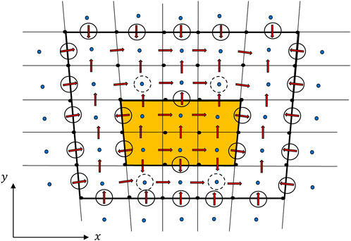
FIGURE 1. 2D sketch of a staggered mesh on a plasma domain with an interior object (in orange). The location of the discretized equations affected by the boundary conditions on currents is represented with circles; solid circles refer to the normal electric currents imposed explicitly, while dashed circles refer to current continuity equations, in which the normal current of the adjacent material cell face is imposed as a known right-hand side. Ghost cells surround the surface boundaries of the domain, except for the edges and corners, where they are not needed.

The use of an FV approach to solve Eq. 6 for the electric current guarantees that the scheme is conservative, without any numerical electric current sink/source, as is the case of the FD method. However, since the unknowns are located at staggered points, interpolation is needed to go from mesh nodes to face or cell centers and vice versa. Finally, centered FD schemes of 2nd-order accuracy are applied everywhere for the gradient discretization of Eq. 4, thanks to the use of ghost cells, as shown in Figure 1. Ghost cells are employed to apply boundary conditions on the external surface of the domain, so they are placed corresponding to each external cell face of the domain, thus surrounding it except for the edges and corners of the 3D domain.

We let vectors {j} and {j_i} group the three components of the electric and ion current density vectors at all cell face centers and the vector {Φ} group, the thermalized potential at all cell centers. We let n_nodes, n_cells, and n_faces represent the total number of nodes, cells (including ghost ones), and faces of the 3D computational mesh, respectively. Then, Eq. 4 can be discretized as

$\left\{\mathit{j}\right\}=-{\sigma }_{\text{e}}\left[H\right]\left[\nabla \right]\left\{\mathrm{\Phi }\right\}-\left[H\right]\left\{{\mathit{j}}_{\text{c}}\right\}+\left\{{\mathit{j}}_i\right\},(13)$

while the matrices [∇] and [H] are explained in the following.The (3n_faces × n_cells) matrix [∇] permits to go from Φ values at the surrounding cell centers to Φ physical derivatives at cell face centers, expressed as in Eq. 10. Thus, [∇] includes the components of the Jacobian matrix $\mathcal{J}$. Figure 2A shows the considered stencil for in-plane derivatives (i.e., along a direction parallel to the cell face plane) appearing in the matrix [∇]. First, Φ is averaged from four cell centers to obtain it at the two sides of the considered cell face, and then, a central scheme is applied. It should be noted that the Φ values of the two involved central cell centers appear with a + sign in one average and with a − sign in another, so they cancel out in the derivative (the number of non-zero entries in the matrix is, thus, only four). Figure 2B shows the same in-plane derivative, but at a corner/edge boundary face, employing the same centered scheme as for internal faces while considering the absence of ghost cells along the domain edge. The (3n_faces × 3n_faces) matrix [H], on the other hand, contains the coefficients derived from $\mathcal{K}$ entries.

FIGURE 2

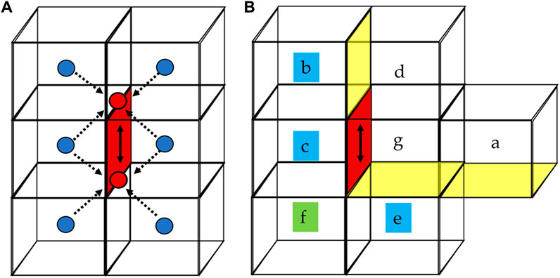
FIGURE 2. (A) Stencil for the in-plane face derivative (at the red face location, along the direction of the black arrow), employing six cell centers (blue dots). Red dots are at the location of the two averages over the four adjacent cell centers. A centered FD scheme is then applied to the red dots to obtain the potential derivative, analogously to the across-face derivatives. (B) Stencil for in-plane face derivatives at domain corner/edge boundary faces. Yellow (and the red) faces show simulation boundary faces. Ghost cells “b,” “c,” and “e” are highlighted in blue. A non-existent cell “f” exists since we are near a domain edge, and its contribution is expressed as a function of the other cells, specifically a trivial linear extrapolation from the location “g” is applied, and the derivatives at “g” along the horizontal and vertical directions are obtained with centered schemes from cells “a–c” and “d–e”, respectively.

Specifically [H] is the matrix relating {j_x, j_y, and j_z} to the physical derivatives of the thermalized potential {∂Φ/∂x, ∂Φ/∂y, and ∂Φ/∂z}. Therefore, it is shaped as

$\left[H\right]=\left[\begin{array}{ccc}\hfill {\left[\mathcal{K}\right]}_1\hfill & \hfill 0\hfill & \hfill 0\hfill \\ \hfill 0\hfill & \hfill {\left[\mathcal{K}\right]}_2\hfill & \hfill 0\hfill \\ \hfill 0\hfill & \hfill 0\hfill & \hfill \dots \hfill \end{array}\right],(14)$

with ${[\mathcal{K}]}_{i=\mathrm{1,2},\dots }$ as the conductivity tensor from Eq. 5 referring to the i^th face center location. The [H] matrix then has three non-zeros per row and three non-zeros per column at maximum.

If {j_n} represents the vector containing, for each face, the electric current density normal to it, then, we can introduce a rectangular matrix [F] of size n_faces × 3n_faces, such that {j_n} = [F]{j}. Introducing this into Eq. 13 yields

$\left\{j_{\text{n}}\right\}=-{\sigma }_{\text{e}}\left[F\right]\left[H\right]\left[\nabla \right]\left\{\mathrm{\Phi }\right\}-\left[F\right]\left[H\right]\left\{{\mathit{j}}_{\text{c}}\right\}+\left[F\right]\left\{{\mathit{j}}_{\text{i}}\right\}.(15)$

At the same time, Eq. 6 and BCs can be easily discretized as

$\left[R\right]\left\{j_{\text{n}}\right\}=\left\{C\right\},(16)$

where {C} contains source/sink terms (at cell centers) or known values of j_n at the boundary cell face centers, and the (n_cells × n_faces) matrix [R] is defined as

$\left[R\right]=\left[\begin{array}{c}\hfill \left[A\right]\hfill \\ \hfill \left[BJ\right]\hfill \end{array}\right],(17)$

where [A] represents the continuity matrix (referred only to plasma cells, excluding the 3D object inner cells touching a plasma cell, and ghost cells beyond the external boundary), and [BJ] groups the BC equations on known normal electric currents at all boundary cell faces (be they external or material boundaries). The continuity equations and BCs are actually interlayered, following the employed cell numbering system, which includes ghost cells. Referring to Figure 1, at the row index corresponding to a ghost cell, the BC relative to the boundary face belonging to that ghost cell is applied. Additional BCs on internal objects, on the other hand, are implemented by substituting the continuity equation of the cell right inside the object (with respect to the considered face) with an explicit BC on j_n. At the edges of internal objects, if the internal cell row has already been used to impose explicitly a normal current density, an external plasma cell continuity equation is modified by bringing to the right-hand side the known current density of the considered face (see dashed circles in Figure 1).

Substituting Eq. 15 into Eq. 16, the linear system

$-{\sigma }_{\text{e}}\left[R\right]\left[F\right]\left[H\right]\left[\nabla \right]\left\{\mathrm{\Phi }\right\}=\left\{C\right\}+\left[R\right]\left[F\right]\left[H\right]\left\{{\mathit{j}}_{\text{c}}\right\}-\left[R\right]\left[F\right]\left\{{\mathit{j}}_{\text{i}}\right\}(18)$

is finally obtained. Thus, the final matrix of the system to be solved is [M] = −σ_e [R] [F] [H] [∇]. This is a square matrix of size n_cells × n_cells, and its maximum rank is obtained by imposing the Dirichlet condition on Φ at one or more cell centers. The BCs on the thermalized potential, contrary to those on the electric current density, are directly applied at the level of this final matrix [M]. For instance, at a cathode injection surface, continuity equations of the cells right inside the cathode surface are substituted with the condition on Φ, expressed as an average potential over internal and external cells.

The developed code first builds the elementary matrices [R], [F], [H], and [∇]; then, it performs their sparse products with the vectors {j_i} and {j_c} at each integration time step and solves for the obtained linear system with a PARDISO [28] direct solver.

Although Φ and j_n are obtained at cell and face centers, respectively, they are later interpolated to mesh nodes for the computation of ϕ and for post-processing purposes.

The maximum number of non-zeros per row of the matrix [M] is equal to 19, which is the same as in the FD scheme. For a given mesh, since the number of non-zero entries and the size of the matrix are the same, the two methods do not show relevant differences in terms of the CPU time.

In the following sections, the aforementioned FV scheme is compared with the previous FD approach for two plume configurations with different physical properties, aiming at testing different aspects of the numerical approach. The comparison between the numerical methods is carried out at the first fluid solution for Φ, in order to avoid propagation, in time, of the solution differences. The considered simulation parameters are summarized in Table 1.

TABLE 1

TABLE 1. Simulation setup parameters and variables for both physical scenarios. The reference electron density n_e0 represent the quasi-neutral density at the reference node for electrons, produced by the injected ion profile.

4 Unmagnetized scenario benchmark

Scenario 1 considers a non-neutral unmagnetized plasma plume that interacts with a S/C; an ion beam is emitted by an ion thruster and neutralized in both the electric charge and current using an external cathode. In this first scenario, taken from [11], a non-linear Poisson solver is employed in non-neutral regions of the domain (i.e., inside the spatially resolved plasma sheaths near the material boundaries) and the considered internal objects are the spacecraft main body, a thruster case with an accelerating grid on top, a cathode keeper, and two solar arrays. Figure 3A shows the employed mesh for both the PIC and electron submodels, including the mentioned 3D material objects. The relevant physical and computational simulation parameters are summarized in the left column of Table 1. Ions are injected from both the thruster and neutralizer exit planes with a Gaussian radial density profile and a mean injection velocity along the +z direction. Although only parameters for Xe⁺ are shown, the simulation features the injection of doubly charged ions from the thruster exit plane; a Xe⁺⁺ mass flow of 0.105 mg/s is injected with a velocity of 55.3 km/s. Moreover, a fraction of 5% of the total neutralizer mass flow is emitted in the form of singly and doubly charged ions from a thermal reservoir at 0.2 and 0.4 eV, respectively, and a neutral mass flow of 0.27 mg/s is injected from the thruster exit plane (corresponding to a thruster mass utilization efficiency equal to 90%).

FIGURE 3

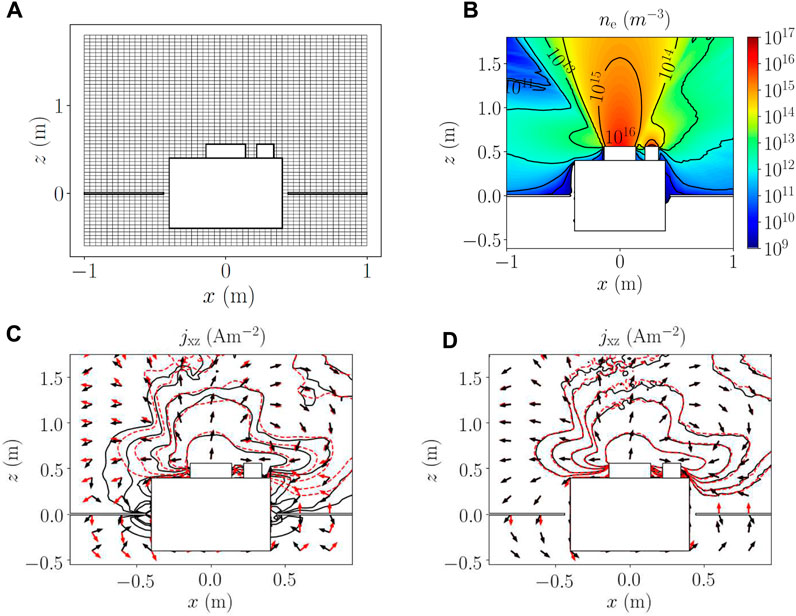
FIGURE 3. Cross sections at y = 0 (through the satellite center) of (A) employed mesh for the unmagnetized scenario 1, (B) electron density steady-state profile, and (C,D) obtained electric current density j_xz isolines and direction (shown by the arrows) for the FD (black solid lines) and FV schemes (red dashed lines), respectively. In all subplots, the S/C body is shown by the large square, while the thruster case and the neutralizer are shown by the large and small rectangles on the top S/C surface, respectively. Thin solar panels are placed on the sides of the S/C body, at z = 0. In subplot (A), one out of every two nodes is shown for the sake of clarity. In subplots (C) and (D), the electric current isolines, from the periphery to the near plume region, refer to values of 0.1, 0.2, 0.5, 1.0, and 5.0 A/m². Electric current plots refer to solutions obtained with (C) coarse (dx, dy, and dz = 4 cm) and (D) fine meshes (dx, dy, and dz = 2 cm).

The satellite ground (including the cubic body, thruster case, and the back face of the solar arrays), the cathode external surface, and the most external grid of the thruster are modeled as conductive objects, while the front face of the solar arrays is modeled as a dielectric object [11]. The external boundaries of the computational domain feature a local current-free condition, j_n = 0. At the surface of material objects, a local condition on j_n is imposed, with a value depending on the surface type; a metallic surface features a locally non-zero electric current density, while a dielectric surface features j_n = 0. On the cathode emission surface, on the other hand, the Dirichlet condition Φ = 0 is applied so that the required cathode current I_C arises automatically from satisfying the global electric current continuity. A spatial smoothing of PIC inputs for the fluid equations over two nodes is also applied, to mitigate the noise.

To illustrate the expansion of this unmagnetized plume, Figure 3B shows the map of n_e at the steady state (from the FV solution with the finest mesh). Insights into the plume physics can be found in [11]. Here, the focus is on the comparison between the two numerical approaches.

The electric current density $j_{\text{xz}}=\sqrt{j_{\text{x}}^2+j_{\text{z}}^2}$ isolines and the direction in the plane x − z (y = 0) obtained with the two numerical schemes are compared in Figures 3C, D, for two different mesh resolutions. The electric current j goes from the thruster exit plane (larger rectangle) to the cathode exit plane (smaller rectangle) and quickly reduces to zero farther downstream. As the mesh becomes fine enough [subplot (d)], the two schemes agree almost perfectly in both the magnitude and current direction. However, in the coarser mesh case [subplot (c)], the FV method seems to perform much better. The FV solution is nearly the same as that obtained with the finer mesh, while the FD solution changes significantly (in both magnitude and direction). This is confirmed in Table 2, which reports, for both numerical schemes and meshes, the electric current through the cathode, I_C, and the corresponding numerical continuity error ${\epsilon }_{\text{I}}={\sum }_k{I}_k/\left|I_{\text{C}}\right|$, where I_k refers to the electric current through a generic object k (including the cathode), which is positive/negative if emitted/absorbed, respectively. The cathode electric current (negative as it “enters” the cathode) barely varies with resolution in the FV approach, while it changes significantly in magnitude (three times as much) in the FD scheme. Regarding ɛ_I, it is lower than 1% in the FV staggered scheme and is actually different from zero due to the spatial smoothing of the PIC inputs, which introduces small inaccuracies in the surface variables. In the FD case, on the other hand, it is significantly larger and decreases with the cell size, as expected.

TABLE 2

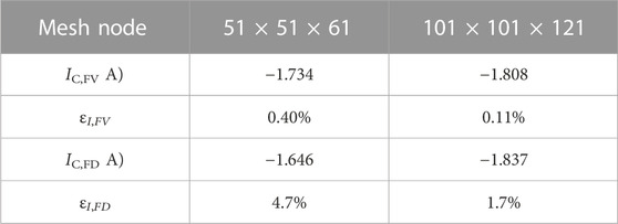
TABLE 2. Electric currents at the cathode and their global error for FV and FD schemes.

The better fluid solution in the FV approach leads to a better coupling with the electric circuit and non-neutral solver models. This is an advantage when it comes to detecting stray currents in objects, as carried out in [29]. Stray currents are relevant as they contribute to S/C charging, an issue of high interest in the field of plasma interaction with the space environment or even in ground facility characterization. These currents are typically small, so if the numerical scheme is affected by a current continuity error, the code is not able to resolve them accurately. In summary, when dealing with objects and even in the absence of magnetic fields, the staggered FV approach, being more natural since it obtains currents at material cell faces rather than at the nodes, is much more robust, and its solution converges much faster with the mesh resolution.

5 Application to a geomagnetic plume expansion scenario

In this section, the new FV scheme is compared against the previous FD approach for a scenario featuring an initially current-free plasma plume expanding in a magnetized environment (scenario 2).

5.1 Simulation settings

In this scenario, taken from [4], the plasma is assumed to be quasi-neutral everywhere, and electron magnetization is due to a background uniform geomagnetic field of 0.5 G along the +x direction (i.e., toward the reader). All relevant physical and computational simulation parameters are summarized in the right column of Table 1, while Figure 4A shows an x = 0 cross section (through the plume centerline) of the employed non-uniform conically expanding mesh for both the PIC and electron submodels. This choice permits us to reduce the statistical noise downstream due to the PIC. Only singly charged ions are injected from the z = 0 cross section with a radial Gaussian density profile and a mean velocity along the z direction. The injection surface is circular, with a maximum radius of 0.20 m, while the 95% ion current radius is assumed to be 0.14 m. For the case of Table 1, the injected Xe⁺ mass flow corresponds to a total ion-injected current I_inj,i = 1.724 A. Since very large values of the Hall parameter still pose problems of numerical convergence [4], a uniform neutral background density n_n is included and is used to limit the maximum Hall parameter in this numerical study.

FIGURE 4

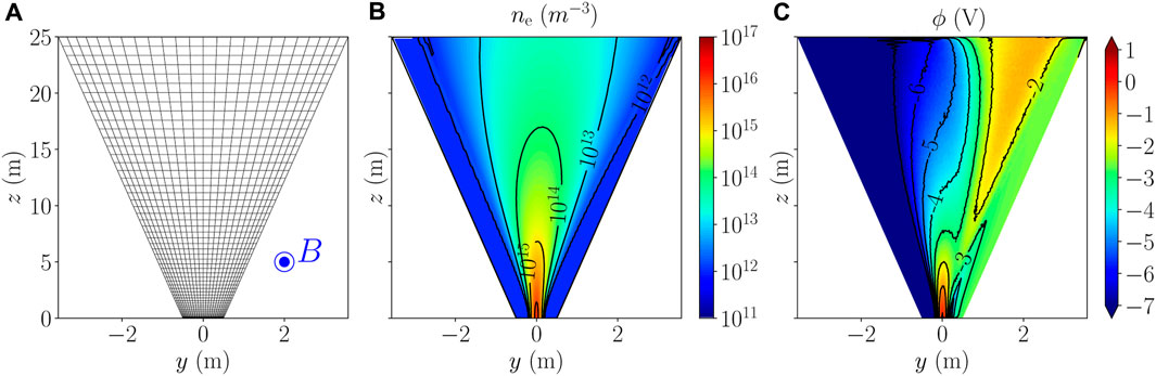
FIGURE 4. Cross sections at x = 0 of the (A) employed mesh for the magnetized scenario 2, with the blue dot representing the +x magnetic field vector coming out of the plane, (B) steady-state electron density, and (C) steady-state electric potential. The results of subplots (B,C) are obtained with the FV staggered scheme using the finest mesh. In subplot (A), one out of every five nodes is shown along both directions.

Regarding BCs, all external boundaries of the computational domain feature a local current-free condition j_n = 0. The Dirichlet condition Φ = 0 is applied only at the reference node for polytropic electron properties, i.e., at x = y = z = 0, where ϕ = 0, T_e = T_e0, and n_e = n_e0. The plume injected into the domain is already locally current-free so that no external neutralizer is included in the simulation.

5.2 Results comparison and discussion

Figures 4B, C show the electron density and electric potential steady-state profiles (from the FV solution with the finest mesh) to illustrate the geometry of the plasma expansion in this physical scenario, respectively. The downstream potential gradient that arises opposes the Lorentz force on ions so that no net plume deflection occurs. The resulting effect is a compression of the plume z cross section along the direction y, which is perpendicular to both the plume centerline (z) and the magnetic field direction (x). Further insights into the involved physics can be found in [4].

Figures 5A–D show a comparison of the electric current density in-plane component magnitude $j_{\text{yz}}=\sqrt{j_{\text{y}}^2+j_{\text{z}}^2}$ in the meridional plane x = 0 obtained with the two numerical schemes, in terms of isolines and direction for a varying maximum Hall parameter χ_max (along each row, increasing from the left to the right) and mesh resolution (along the columns, increasing from top to bottom). Additional intermediate cases in terms of the maximum Hall parameter and mesh resolution can be consulted on demand to authors.

FIGURE 5

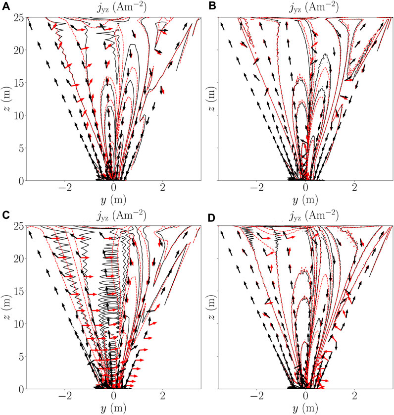
FIGURE 5. Comparison at x = 0 of the electric current density j_yz isolines and direction (shown by arrows) with the FD (black solid lines) and FV methods (red dashed lines) obtained with the (A,C) coarsest and (B,D) finest mesh. (A,B) refer to χ_max = 35, and (C,D) refer to χ_max = 100. The electric current isolines, from the periphery to the plume core and the injection region, assume values of 0.01, 0.1, 0.5, 1.0, and 5.0 A/m².

As explained in [4] and referring to Figure 5, the magnetic field induces an electric current loop in the yz plane, with a positive current tube on the left and a returning negative current tube on the right. In particular, the current flowing in these tubes increases slightly with the Hall parameter (i.e., from the left to the right). Noticeably, larger oscillations appear in the FD approach, and these clearly reduce for finer meshes and lower maximum Hall parameters. Therefore, a mesh resolution that is enough at a low χ_max value might be inappropriate at a larger χ_max value. When this happens, the solution seems to oscillate around an average value. These oscillations are not associated with the global continuity error (i.e., the artificial current rising at the Dirichlet node, whose origin is explained in Supplementary Appendix SB) but are due to the stencil used, and the fact that the unknowns are solved in collocated grids. A non-staggered mesh is what produces these sawtooth “cell-size” chequerboard oscillations, which are still a solution of the discretized equations. The staggered FV scheme, on the other hand, is more robust, but nonetheless, it is still subject to some oscillations in very stiff problems like this, due to both ill-conditioning and the gradient scheme, which involves the contribution of more cells. It should be noted that both numerical schemes are affected by flux discretization errors which depend on the stencils employed and the number of surrounding points contributing to the discretized derivatives. In both cases, higher-order schemes would mitigate these errors but the computational burden would increase. The adopted schemes are considered adequate and are commonly used in these kinds of problems. Moreover, since numerical diffusion is absent in this scenario (with the magnetic field parallel to a mesh axis), errors in flux discretization are expected to be small. The FV and FD methods tend to almost coincide as the mesh resolution increases; this also constitutes the validation of the physical solution of the newly implemented FV approach in EP2PLUS.

The staggered FV approach, thus, converges quicker at coarser meshes, and more importantly, it is not affected by a global continuity error like the FD approach. Table 3 shows the value of the integrated electric current $I_{\text{z}}^{+}$ through the positive electric current tube (where j_z >0) at the z = 10 m cross section for both numerical schemes and for all the maximum Hall parameters and mesh resolutions investigated. The FV method is capable of reproducing this global physical property already with the coarsest mesh (with an underestimation of less than 1%), while the FD results show a much larger dependence on the mesh resolution.

TABLE 3

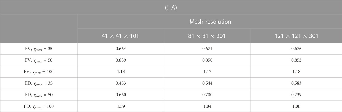
TABLE 3. Comparison of the integrated electric current $I_{\text{z}}^{+}$ flowing through the positive current tube of the diamagnetic loop, obtained with the two numerical schemes, for different values of χ_max and mesh resolutions, in scenario 2.

In the magnetized scenario 2, when using the FD scheme, the Hall parameter must be limited to values not larger than 50–100 in order to maintain an acceptable quality in the solution for reasonable mesh resolutions. As mentioned previously, this is achieved here through an ad hoc neutral density background to increase the minimum electron collisionality. This limitation is mainly due to the non-conservativeness of the FD approach, which does not exactly solve the divergence equation. The overall consequence of the discretization error is that, at the Dirichlet node, the local electric current density in the direction normal to the boundary is not 0, and its integrated value I_Dir (with the surface associated with the node) quantifies the global continuity error. It turns out that it is almost inversely proportional to the square of the number of nodes in each mesh direction, confirming that it is ultimately related to FD truncation errors, as can be seen in Figure 6. Here, ${\epsilon }_{I,FD}=\left|I_{\text{Dir}}\right|/I_{\text{inj,\hspace{0.17em}i}}$, and it represents the relative error (normalized with the total injected ion current) and $\tilde{N}$ represents the number of nodes along each direction normalized with the coarsest mesh case (for which $\tilde{N}=1$). It should be noted that the artificial current can reach values that are even larger than the injected ion current, for the lowest resolution case with the highest maximum Hall parameter. We point out, however, that simulations in [4] had a quite lower global continuity error, in the order of 5%, since they considered a more carefully selected mesh with an increasing resolution close to all boundaries (where physical gradients are the largest), a fact that has not been adopted here since the focus is on highlighting the advantages of the new FV scheme and in showing the origin and consequences of the discretization errors associated with the FD approach.

FIGURE 6

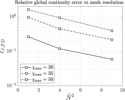
FIGURE 6. Global continuity error in FD simulations for scenario 2, as a function of the square of the normalized number of nodes along one direction, for different maximum Hall parameters.

5.3 Effects of the maximum transport anisotropy on the circulating electric current

The conservativeness of the FV method has enabled an extended analysis (compared to what was carried out in past studies [4]) on the effects of the neutral background on the obtained physical solution. A set of simulations with a varying neutral background density to reproduce a maximum Hall parameter of 20, 35, 50, 100, 250, 400, and 500 have been considered, with the conservative FV scheme and the highest mesh resolution. It should be noted that the previous studies with the FD scheme had been carried out only for χ_max ≤100. Indeed, the FD formulation failed to converge to a solution in the extended range of χ_max values, even with the highest mesh resolution. A higher resolution was needed for the FD scheme to converge (to a smooth solution not affected by oscillations and a low continuity error) and would require excessive computational times. The integrated positive electric current at the z = 10 m cross section, normalized with the total ion-injected current I_inj,i, is computed and plotted as a function of χ_max in Figure 7.

FIGURE 7

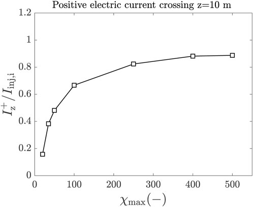
FIGURE 7. Integrated current flowing through the positive current tube (j_z >0) at z = 10 m as a function of the maximum Hall parameter (non-dimensional). Simulations results are obtained with the FV approach and the finest mesh resolution.

As partially predicted in [4], the integrated current tends to clearly saturate with the maximum Hall parameter and tends to a value that is slightly lower than the injected ion current. Figure 8 shows the local effects of the increasing χ_max value on the electric current density, and the shape and magnitude of the diamagnetic loop. Higher magnetization levels, χ, generate a larger electric current flowing in the tubes and, hence, a bigger deformation of the latter in the xy plane. In particular, the asymmetry between the positive and negative current tubes becomes more evident, with the positive current tube getting wider and the negative current tube shrinking. Nevertheless, the general trend of a saturation of such effects, anticipated in [4], is confirmed here for a much larger variation range for χ.

FIGURE 8

FIGURE 8. Comparison of FV solutions at χ_max = 50 (solid black line), χ_max = 100 (dotted blue line), and χ_max = 250 (dashed red line), in terms of (A) electric current density j_yz isolines (0.4, 1.0, 2.0, and 5.0 A/m² from the periphery to the plume core and injection region) at x = 0 m and (B) electric current density absolute value |j_z| isolines (0.1, 0.2, and 0.7 A/m² from the periphery to the inner region of the two current tubes) at z = 12.5 m. In subplot (B), a plus and minus sign give the direction of j_z in the current tubes.

The aforementioned study constitutes a further validation and successful application of the advantages and capabilities of the FV scheme. Due to the conservativeness of the FV scheme, no artificial source of current is present, and the integrated current in the positive current tube (j_z >0) is exactly equal and opposite to the one flowing through the negative current tube (j_z <0) for continuity.

6 Conclusions and future work

This work has presented the upgrade of the numerical scheme for solving an electron magnetized fluid model within the 3D hybrid simulation code EP2PLUS. The new finite volumes scheme has been compared with the original finite differences scheme of the code for two physical scenarios: the plasma environment around a spacecraft created by the plasma plume of an ion thruster [11] and the expansion of a current-free plasma plume affected by the geomagnetic field [4]. The two physically and computationally different scenarios were specifically considered to test many critical points, such as boundary conditions with 3D objects, magnetization effects, non-neutrality effects, or different shapes of the structured meshes (rectangular uniform but also non-uniform and non-rectangular ones). The discretized form of the equations, the final form of the involved matrices, and the considered BCs have been described for the two schemes. They have been benchmarked for varying mesh resolutions and, in the magnetized scenario, for different maximum Hall parameters. Although at a very large mesh resolution, both schemes tend to give the same physical solution, the weaknesses of the FD approach and the practical advantages of the new FV scheme have been highlighted. First, the FV scheme presents a conservative and more natural implementation of the first-order electron fluid equations and their boundary conditions, allowing us to precisely characterize variables as fluxes at their natural physical location, i.e., at the surface boundaries of the domain and internal objects. Second, the use of a staggered mesh is shown to mitigate the chequerboard issue, evident in some FD solutions. Third, it presents less spurious errors (the FD solution is corrupted by a global continuity error that is absent in FV). Fourth, the FV scheme attains a similar quality of the solution with a coarser mesh, thus allowing either a larger saving in the computational time or a more accurate solution with similar computational efforts. Fifth, in the case of a magnetized plume, it can deal with much larger values of the Hall parameter (i.e., higher magnetization), where the FD scheme does not converge. This has permitted the extension to higher Hall parameters of the study in [4], confirming the saturation trend in the electric current circulating inside diamagnetic loops. Nonetheless, the FV approach is still sensitive to the ill-conditioned nature of a 3D magnetized problem. Convergence continues to be problematic at very high electron transport anisotropy, meaning Hall parameters of the order of 100–1000, depending on the particular scenario. Further improvements would be beneficial at domain boundary edges and corners, in order to have more homogeneous schemes and to mitigate any artificial boundary effect. Still on the numerical side, future work must check the absence of numerical diffusion when applying oblique and non-uniform magnetic topologies. This can be carried out by comparing the plasma responses obtained with the Cartesian-type meshes of EP2PLUS and the magnetic field aligned meshes of similar hybrid codes, such as HYPHEN [30]. The use of a Cartesian-type mesh seems mandatory if the induced magnetic field effects are considered relevant, since the total magnetic field is not known a-priori. Once validated, for the new FV scheme, the physical capabilities of EP2PLUS can be improved. First, the extension of the stationary plume model presented here to plumes with low- or mid-frequency dynamics is almost immediate since the PIC formulation of heavy species is already time-dependent, and the electron response is quasi-stationary below megahertz frequencies. Second, and of high practical interest, is the ongoing validation of a new version of EP2PLUS, solving the electron-full energy equation (instead of applying an empirical polytropic closure) [18]. In this new version, the new FV scheme is applied to both the pair of electron continuity and momentum (i.e., Ohm’s) equations, and the pair of energy and heat-flux Fourier equations. All these numerical and physical advances are, for instance, needed to apply EP2PLUS to the study of Hall thruster plumes, with their complex magnetic topologies, current neutralization, and active collisionality [15]. Lastly, the new FV scheme has already been successfully applied to a scenario featuring the expansion of an electrodeless thruster plume within a magnetic nozzle [31] and contributed to gaining physical insight into the governing mechanisms.

Data availability statement

The raw data supporting the conclusion of this article will be made available by the authors, without undue reservation.

Author contributions

AM: conceptualization, methodology, software, and writing—original draft. FC: software, conceptualization, methodology, supervision, and writing—original draft. EA: methodology, supervision, and writing—review and editing.

Funding

The author(s) declare that financial support was received for the research, authorship, and/or publication of this article. The research has been funded by the H2020 CHEOPS MEDIUM POWER project (grant agreement ID: 101004226). The contribution of FC to code development was completed while he was affiliated to Universidad Carlos III de Madrid, while most of his text contribution was completed when he was affiliated to the Institute for Plasma Science and Technology (ISTP-CNR), Bari, Italy.

Acknowledgments

The authors would also like to thank Mario Merino and Jiewei Zhou for support and counsel during the developments of this work.

Conflict of interest

The authors declare that the research was conducted in the absence of any commercial or financial relationships that could be construed as a potential conflict of interest.

Publisher’s note

All claims expressed in this article are solely those of the authors and do not necessarily represent those of their affiliated organizations, or those of the publisher, the editors, and the reviewers. Any product that may be evaluated in this article, or claim that may be made by its manufacturer, is not guaranteed or endorsed by the publisher.

Supplementary material

The Supplementary Material for this article can be found online at: https://www.frontiersin.org/articles/10.3389/fphy.2023.1286345/full#supplementary-material

References

1. Ahedo E. Plasmas for space propulsion. Plasma Phys Controlled Fusion (2011) 53:124037. doi:10.1088/0741-3335/53/12/124037

CrossRef Full Text | Google Scholar

2. Goebel D, Katz I. Fundamentals of electric propulsion: ion and Hall thrusters. Pasadena, CA: Jet Propulsion Laboratory (2008).

Google Scholar

3. Merino M, Ahedo E. Magnetic nozzles for space plasma thrusters. In: JL Shohet, editor. Encyclopedia of plasma technology, 2. Taylor and Francis (2016). p. 1329–51.

Google Scholar

4. Cichocki F, Merino M, Ahedo E. Three-dimensional geomagnetic field effects on a plasma thruster plume expansion. Acta Astronautica (2020) 175:190–203. doi:10.1016/j.actaastro.2020.05.019

CrossRef Full Text | Google Scholar

5. Korsun A, Tverdokhlebova E. Geomagnetic field perturbation by a plasma plume. In: 25th international electric propulsion conference (fairview park, OH. Fairview Park, OH: Electric Rocket Propulsion Society (1997).

Google Scholar

6. Korsun A, Tverdokhlebova E, Gabdullin F. Mathematical model of hypersonic plasma flows expanding in vacuum. Comp Phys Commun (2004) 164:434–41. doi:10.1016/j.cpc.2004.06.078

CrossRef Full Text | Google Scholar

7. Cichocki F, Merino M, Ahedo E. Spacecraft-plasma-debris interaction in an ion beam shepherd mission. Acta Astronautica (2018) 146:216–27. doi:10.1016/j.actaastro.2018.02.030

CrossRef Full Text | Google Scholar

8. Hockney R, Eastwood J. Computer simulation using particles. Boca Ratón, FL: CRC Press (1988).

Google Scholar

9. Wang J, Han D, Hu Y. Kinetic simulations of plasma plume potential in a vacuum chamber. IEEE Trans Plasma Sci (2015) 43:3047–53. doi:10.1109/tps.2015.2457912

CrossRef Full Text | Google Scholar

10. Taccogna F, Minelli P. Three-dimensional particle-in-cell model of hall thruster: The discharge channel. Phys Plasmas (2018) 25:061208. doi:10.1063/1.5023482

CrossRef Full Text | Google Scholar

11. Cichocki F, Domínguez-Vázquez A, Merino M, Ahedo E. Hybrid 3D model for the interaction of plasma thruster plumes with nearby objects. Plasma Sourc Sci Tech (2017) 26:125008. doi:10.1088/1361-6595/aa986e

CrossRef Full Text | Google Scholar

12. Wartelski M, Theroude C, Ardura C, Gengembre E. Self-consistent simulations of interactions between spacecraft and plumes of electric thrusters. In: 33rd International Electric Propulsion Conference (Washington D.C.; October 7-10; Fairview Park, OH. Electric Rocket Propulsion Society (2013). paper 2013-73.

Google Scholar

13. Cheng S, Santi M, Celik M, Martínez-Sánchez M, Peraire J. Hybrid PIC-DSMC simulation of a Hall thruster plume on unstructured grids. Comp Phys Commun (2004) 164:73–9. doi:10.1016/j.cpc.2004.06.010

CrossRef Full Text | Google Scholar

14. Brieda L, Pierru J, Kafafy R, Wang J. Development of the DRACO code for modeling electric propulsion plume interactions. In: 40th joint propulsion conference and exhibit. Reston, VA: American Institute of Aeronautics and Astronautics (2004). paper 2004-3633.

CrossRef Full Text | Google Scholar

15. Cichocki F, Domínguez-Vázquez A, Merino M, Fajardo P, Ahedo E. Three-dimensional neutralizer effects on a Hall-effect thruster near plume. Acta Astronautica (2021) 187:498–510. doi:10.1016/j.actaastro.2021.06.042

CrossRef Full Text | Google Scholar

16. Merino M, Cichocki F, Ahedo E. A collisionless plasma thruster plume expansion model. Plasma Sourc Sci Tech (2015) 24:035006. doi:10.1088/0963-0252/24/3/035006

CrossRef Full Text | Google Scholar

17. Ortega A, Katz I, Mikellides I, Goebel D. Self-consistent model of a high-power Hall thruster plume. IEEE Trans Plasma Sci (2015) 43:2875–86. doi:10.1109/tps.2015.2446411

CrossRef Full Text | Google Scholar

18. Modesti A, Cichocki F, Zhou J, Ahedo E. A 3D electron fluid model with energy balance for plasma plumes. In: Iepc 2022. Boston, Massachusetts, United States: IEPC (2022). June 19-23.

Google Scholar

19. Ahedo E. Using electron fluid models to analyze plasma thruster discharges. J Electric Propulsion (2023) 2:2. doi:10.1007/s44205-022-00035-6

CrossRef Full Text | Google Scholar

20. Araki SJ, Martin RS, Bilyeu D. Current capabilities of afrl’s spacecraft simulation tool. In: Iepc 2022. Boston, Massachusetts, United States: IEPC (2022). June 19-23.

Google Scholar

21. Magarotto M, Melazzi D, Pavarin D. 3d-virtus: Equilibrium condition solver of radio-frequency magnetized plasma discharges for space applications. Comp Phys Commun (2020) 247:106953. doi:10.1016/j.cpc.2019.106953

CrossRef Full Text | Google Scholar

22. LeVeque RJ. Finite volume methods for hyperbolic problems, 31. Cambridge University Press (2002).

Google Scholar

23. Toro EF, Solvers R. Numerical methods for fluid dynamics: a practical introduction. Berlin, Germany: Springer (1999).

Google Scholar

24. Canuto C, Hussaini MY, Quarteroni A, Zang TA. Spectral methods: Evolution to complex geometries and applications to fluid dynamics. Springer Science and Business Media (2007).

Google Scholar

25. Vinokur M. An analysis of finite-difference and finite-volume formulations of conservation laws. J Comput Phys (1989) 81:1–52. doi:10.1016/0021-9991(89)90063-6

CrossRef Full Text | Google Scholar

26. Domínguez-Vázquez A, Cichocki F, Merino M, Fajardo P, Ahedo E. Axisymmetric plasma plume characterization with 2D and 3D particle codes. Plasma Sourc Sci Tech (2018) 27:104009. doi:10.1088/1361-6595/aae702

CrossRef Full Text | Google Scholar

27. Domínguez-Vázquez A, Zhou J, Sevillano-González A, Fajardo P, Ahedo E. Analysis of the electron downstream boundary conditions in a 2D hybrid code for Hall thrusters. In: 37th International Electric Propulsion Conference; June 19-23; Boston, MA. Electric Rocket Propulsion Society (2022). p. 2022–338. IEPC.

Google Scholar

28. Alappat C, Basermann A, Bishop AR, Fehske H, Hager G, Schenk O, et al. A recursive algebraic coloring technique for hardware-efficient symmetric sparse matrix-vector multiplication. ACM Trans Parallel Comput (Topc) (2020) 7:1–37. doi:10.1145/3399732

CrossRef Full Text | Google Scholar

29. Modesti A, Zhou J, Cichocki F, Domínguez-Vázquez A, Ahedo E. Simulation of the expansion within a vacuum chamber of the plume of a hall thruster with a centrally mounted cathode. In: Space Propulsion Conference 2022; May 9-13. Association Aéronautique et Astronautique de France (2022). 00155.

Google Scholar

30. Domínguez-Vázquez A, Zhou J, Fajardo P, Ahedo E. Analysis of the plasma discharge in a Hall thruster via a hybrid 2D code. In: 36th International Electric Propulsion Conference; Vienna, Austria. Electric Rocket Propulsion Society (2019). IEPC-2019-579.

Google Scholar

31. Cichocki F, Navarro-Cavallé J, Modesti A, Ramírez Vázquez G. Magnetic nozzle and RPA simulations vs. experiments for a helicon plasma thruster plume. Front. Phys. (2022) 10:876684. doi:10.3389/fphy.2022.876684

CrossRef Full Text | Google Scholar