Acoustic noise levels and field distribution in 7 T MRI scanners

Acoustic noise production during Magnetic Resonance Imaging is an important source of patient discomfort and leads to verbal communication problems, difficulties in sedation, and hearing impairment. To address these issues, in this paper we present a systematic characterization of the acoustic field distribution in a MRI cavity in a last generation 7 T scanner, in different spatial locations, with and without a phantom head. Analysis and comparison of various MRI sequences like Echo-planar imaging”, “Gradient echo”, “Spin echo” are carried out. Sound pressure levels are measured using standard statistical descriptors ($L_{eq},$ $L_{mean}$, $L_{90}$, and $L_{mode}$) using two prepolarized free-field microphones measuring pressure levels generated inside scanner cavities in a 50 Hz to 10 kHz range. Acoustic eigenmodes of the cavity are derived numerically in finite element simulations and compared to measurements. Equivalent sound pressure levels exceed 85 dB in the range between 500 and 3,000 Hz, and peak levels are consistently above 100 dB, i.e., the noise levels of 7 T scanners are higher than 3T and 1.5 T counterparts. The presence of the phantom head in the MRI scanner leads to increased noise levels (by 5–10 dB) in its vicinity, as a result of reflections occurring between the head and the bore reflective walls. Numerical finite element simulations allow to extrapolate the noise distribution in the entire cavity and to interpret experimental results and indicate that the frequencies at which the highest noise levels occur correspond to azimuthal or radial resonant modes of the MRI cavity, i.e., with a radially and azimuthally varying pressure field. These results can be useful for the design of future acoustic noise mitigation solutions.

1 Introduction

Magnetic Resonance Imaging (MRI) is a non-invasive 3D imaging procedure largely used in the field of medical diagnostics and follow-up. During an MRI session, magnetic field gradient commutations lead to extremely high acoustic noise levels, which can be a source of discomfort and even of harm for patients [1]. Acoustic noise is generated due to Lorentz forces caused by rapid current variations within the magnetic field gradient coils [2], which produce motion or vibration of the coils as they impact against mountings [3]. Aside from its inconvenience, the presence of strong acoustic noise can influence results of functional MRI measurements performed in the auditory [4], visual, and motor cortex [5], interfering with brain function and changing blood oxygenation level dependent signals [6]. The highest levels of acoustic energy for the most used pulse sequences, i.e., spin-echo, gradient-echo, and variant, are predominantly concentrated at low frequencies [7]. The noise spectrum may also vary according to the type of scanners. For example, Ravicz et al. have measured 1 kHz and 1.4 kHz peaks in 1.5 T and 3 T scanners, respectively [8]. They also showed that other noise sources, such as the cooling pump for the permanent magnet and the room air-handling system, may marginally increase the levels of acoustic noise.

Acoustic noise profiles are closely linked to the MRI pulse sequences and the type of scanners. Standard MRI systems may produce Sound Pressure Levels (SPLs) above the recommended 85 dB level on the linear scale [7] using clinically accepted MRI pulse sequences. In addition, larger gradients are expected to produce higher noise levels. An extensive investigation on the acoustic noise levels for various MRI systems with magnetic field intensity ranging from 0.2T to 3 T indicated acoustic noise to be larger for higher magnetic field intensities [9]. The corresponding values ranged from 82.5 dBA to 118.4 dBA. Higher SPL values were reported in the literature for 4 T MRI scanners, reaching values as high as 130 dB [10]. Open MRI scanners usually reduce acoustic noise, which is amplified in tunnel-configuration designs due to reverberation phenomena [11]. Noise levels are slightly increased when patients are present and may vary by 10 dB or more with respect to the longitudinal position in the scanner [12].

Noise measurement studies in MRI scanners are usually aimed at the development of noise reduction strategies to reduce patient discomfort. Possible solutions to reduce acoustic noise levels may include the redesign of the employed gradient coil in MRI scanners [13]. However, this approach would require significant modifications to the currently used equipment [14]. Approaches which do not require the redesign of the equipment include 1) pulse optimization for quieter imaging sequences, 2) Active Noise Control (ANC), and 3) passive noise control techniques [15]. The reshaping of applied MRI pulse sequences can lead to the suppression of selected frequencies and associated higher harmonics [16]. Although new sequence techniques appear promising in terms of noise reduction, image quality may be affected [17], thereby compromising the diagnostic performance [18]. Sequence conversion algorithms employed to optimize arbitrary MRI schemes also appear to be effective, leading to reductions between 14.4 dBA and 16.8 dBA [19]. However, such techniques may require specialized pulse programming or a considerable increase in the scanning time [20]. ANC techniques [21], on the other hand, introduce antiphase noise to create destructive interference and thus reduce the perceived levels of low-frequency noise [22]. Some examples include feedback adaptive ANC systems showing an average noise power reduction of more than 18 dB [23], hybrid control systems with both feedforward and feedback loops, numerically demonstrating a reduction of 20 dB for 4 T MRI scanner systems at the principal frequency component [24]. Such solutions, however, may be costly and therefore financially unfeasible. Passive noise control solutions such as headphones and earplugs [25] can be used as a simple and economical solution, with a noise reduction between 10 and 30 dB (3). However, the noise attenuation is achieved in a non-uniform manner, mostly attenuating high-frequency components, while also hindering the communication with patients.

Among the various passive noise control solutions proposed to address the issue of noise suppression, acoustic metamaterials [26] seem to be a particularly promising alternative, presenting novel properties not commonly found in natural materials, such as frequency ranges which prevent vibration propagation [27]. More specifically, plate-type structures have been demonstrated as exceptional solutions for the isolation of structure- and sound-borne noise [28, 29]. Examples of applications based on structural wave manipulation include systems with periodically distributed resonators able to achieve high sound transmission loss, including thick plates with resonators [30] and thin plates with arrays of attached resonators [31]. Also, bio-inspired plate structures with optimized two-dimensional periodic arrays of resonators have been shown to yield excellent sound transmission loss for selected frequency ranges [32], also reinforcing the preferred use of locally resonant structures to achieve high sound transmission loss values. Airborne sound attenuation solutions have also been proposed [33] and could provide a promising solution. However, to choose the appropriate noise abatement solution or to effectively design metamaterial structures, it is necessary to have a precise characterization of the acoustic field distribution in the scanner at various frequencies.

The use of numerical models may be of great use in this task. Various simulation approaches have been adopted to model the coil vibrations leading to acoustic noise generation in MRI [34] with many of them based on the Finite Element (FE) method [35–37]. Recent contributions have shown that even linear models can be representative of the involved phenomena if proper corrections are considered [38]. These models, however, must be verified and correlated with the actual test configuration, whose system performance specifications can be determined by performing series of tests with established standards [39]. The resulting measurements can then be used to design optimized structures able to alleviate the problem of noise generation in MRI systems.

In this study, we present a systematic acoustic characterization of a 7 T MRI scanner, considering various spatial locations in the bore hole, various pulse sequences and the presence of a phantom simulating the presence of a patient. The experimental measurements are coupled with a 3D FE model simulating the acoustic field distribution in the scanner, allowing to correlate measurements with resonance modes of the structure. The paper is structured as follows: Section 2 illustrates the experimental and numerical procedures, Section 3 presents measurement and simulation results, and Section 4 provides discussion of results and conclusions.

2 Materials and methods

2.1 Acoustic noise measurements

The acoustic noise measurements were performed in 7 T MRI scanners located in the specialized research centre at La Timone Hospital, Marseille. As illustrated in Figure 1, two configurations of microphone positions were used:

- Configuration A used in-line positions along the axis of the bore and aimed to evaluate the variability of noise levels over the longitudinal (z) axis of the bed plane at a height of 15 cm. The spatial intervals of these measurements were every 20 cm starting with a first calibration of the location at the isocenter of each scanner. A height of 24 cm was also tested at the isocenter.

- Configuration B included the presence of a phantom head and the position of the microphones was set at the level of the ear canal, at 3 cm distance and at a height of 9.5 cm.

FIGURE 1

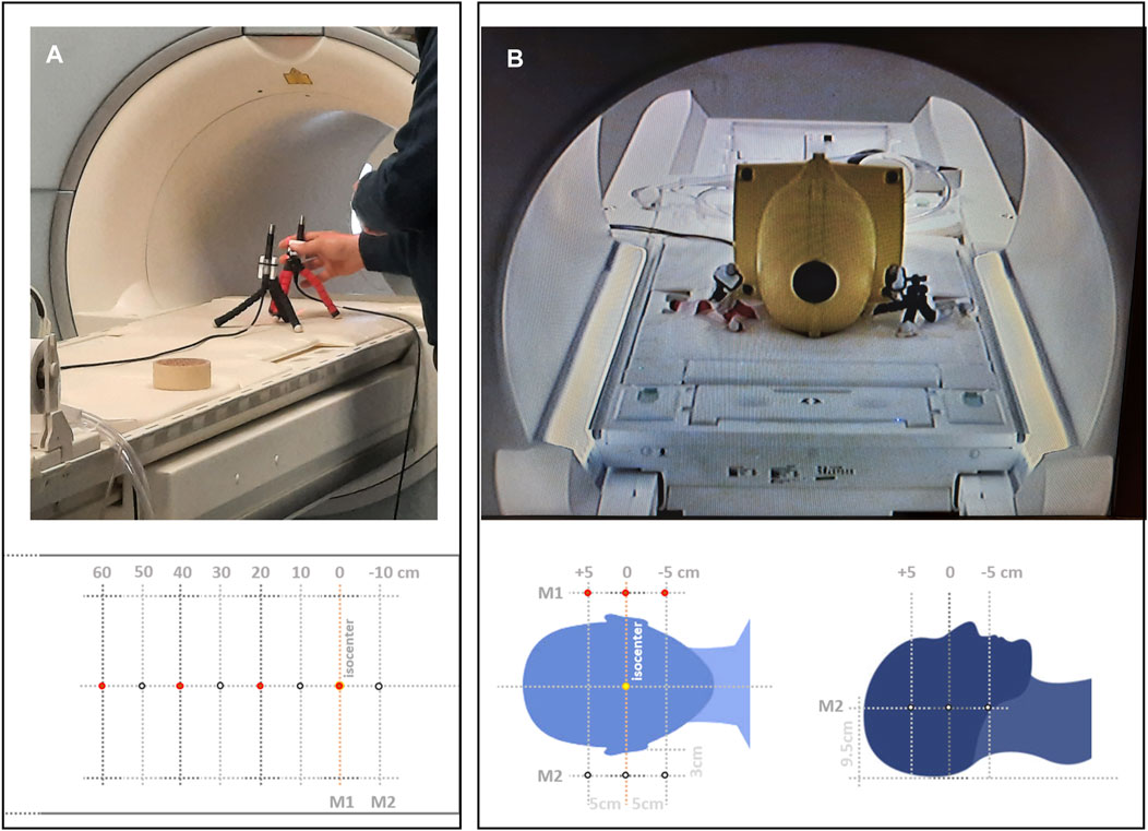
FIGURE 1. Microphone setup with in-line positions (A) and with (B) the phantom head. The microphone positions (M1 and M2) are represented as red and white dots, respectively.

The “Echo-Planar Imaging” (EPI) sequence was used as a reference signal for the comparisons, since it has been associated with the largest noise levels in the literature [3]. However, some comparisons with other sequences, namely, “Gradient Echo” (GRE), and “Spin Echo” (SE), were performed. A summary of all the performed measurements is reported in Table 1, together with the employed sequences. The background noise levels were measured in the MRI scanner room while the scanner was inactive. These measurements were performed to account for the environmental noise levels related to the cooling pump and the room air-conditioning systems.

TABLE 1

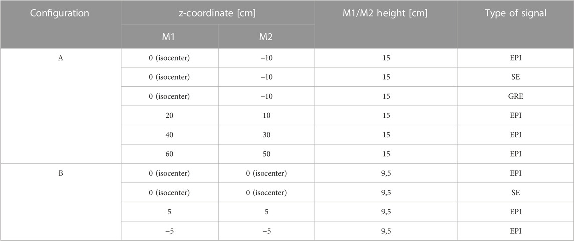
TABLE 1. Summary of the measurements performed in the 7 T MRI scanner. Type of signal sequences are “Echo-planar imaging” (EPI), “Gradient echo sequences” (GRE), and “Spin Echo” (SE).

Two ½″ prepolarized free-field microphones (Type 4189 from B&K) were used for the measurements of the sound pressure levels generated in the MRI scanner. The microphones were equipped with a ZC0032 preamplifier and connected to a two-channel Phonometer (SPL meter, Type 2270 B&K) through AO-0441 cables (Figure 2). The microphones have a high sensitivity over a frequency range of 6.3 Hz–20 kHz. All equipment complies with IEC 61672 class 1. The microphones and cables are compliant with the IEC 61672 class 1 for high precision measurements. This type of setup has also been used in other studies on MRI noise, since it is unaffected by the magnetic field, thanks to appropriate shielding and the absence of any ferrous material [10, 38]. All other instrumentation, except for the microphones and microphone stands, was used in adjacent rooms to that hosting the MRI, due to the high magnetic field and incompatibility with metallic objects.

FIGURE 2

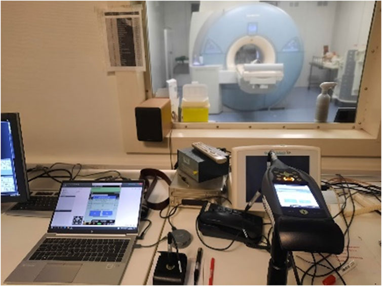
FIGURE 2. Acoustic measurements setup during calibration in the MRI control room.

The measured signals were analysed to determine the L_eq (Equivalent Sound Pressure Level), which is the average sound pressure level during a period of time for each one-third octave band.

2.2 Numerical simulations

Numerical simulations were performed using a FE model representing the acoustic cavity. The cavity consists in a cylindrical bore delimited by a flat bottom on one side. The corresponding diameter and length were specific for each scanner. We show in Figure 3A a schematic of the dimensions for the scanner. The resulting acoustic cavity geometry is shown in Figure 3B, which is henceforth considered as configuration A (model without head phantom). An additional configuration B was also considered, in which the volume of a human head phantom is subtracted from the initial acoustic cavity (Figure 3C). Both models are meshed using linear tetrahedral elements with a typical length of 12 mm, thus yielding at least 6 nodes per wavelength up to 4 kHz. In both FE models, all the boundaries related to the interface between the acoustic cavity and the MRI bore were considered as perfectly rigid, while the edges of the acoustic cavity corresponding to the bore openings were considered as open ends, approximated as zero pressure boundary conditions [40]. Results are presented as relative pressure levels (i.e., atmospheric pressure corresponds to a zero pressure value).

FIGURE 3

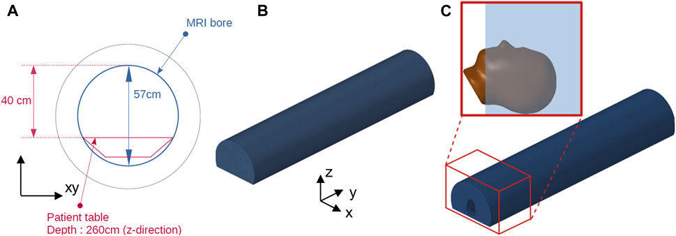
FIGURE 3. (A) Acoustic cavity (bore hole) dimensions for the 7 T scanner. (B) FEM model for the considered acoustic cavity in configuration A (C) FEM model of the cavity in configuration B, obtained by placing the phantom head inside the cavity and subtracting its volume.

3 Results

Before performing the acoustic noise characterization of scanning MRI conditions, the background noise levels were measured and their L_eq were found to be below 75 dB, i.e., mostly negligible (<10 dB) compared to the levels measured subsequently. Further details are provided in the Supplementary Figures SM1, SM2.

3.1 Noise measurements in an empty cavity (configuration A)

Noise levels were first measured for the EPI sequence in the 7 T scanner at a constant height at the isocentre, and varying the position along longitudinal axis. Results are shown in Figure 4, showing the noise levels for each microphone position for the in-line measurements (this is also compared to 1.5 T and 3 T scanners in the Supplementary Figure SM3). In most of the cases, the measured sound level variations with position were below 10 dB, thereby indicating a relatively uniform noise excitation along the whole length of the cavity, and the prevalence of acoustic modes slowly varying along the axis of the cylinder axis, i.e., azimuthal or radial modes, as opposed to longitudinal ones [41]. There is also limited variability in sound levels as a function of microphone height in the cavity (see Supplementary Figure SM4), so that a constant height of 15 cm is chosen for all measurements, given its proximity to mean ear position of patients in the supine position.

FIGURE 4

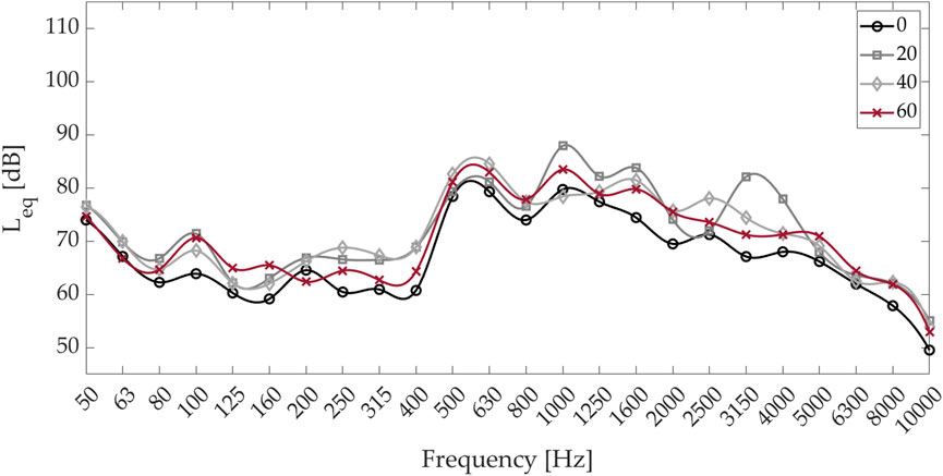
FIGURE 4. EPI sequence sound level variation along the axis of the MRI cavity: L_eq vs. frequency in one-third octave bands, measured at the isocenter for in-line distances of 20, 40, and 60 cm along the z-axis.

In general, equivalent noise levels above 80 dB were mainly reached in the frequency range between 500 Hz and 3 kHz, making this the most critical range to prioritize for noise reduction measures.

A more detailed approach, performed on the basis of a comparative analysis of waveforms, spectrograms and narrow band power density spectra for the three scanners (1.5 T, 3 T, and 7 T) and the corresponding results are reported in the Supplementary Figure SM3.

Three different types of MRI pulse sequences were then compared. These were chosen for their particularly high noise levels. The equivalent sound levels in third-octave bands for EPI, SE, and GRE pulse sequences at the isocenter of the 7 T scanner are shown in Figure 5. A similar trend for the equivalent sound pressure levels has been identified, with the highest levels occurring above 500 Hz. The differences between the three MRI pulse sequences are larger in the range between 80 and 500 Hz. The three MRI pulse sequences display L_peak values above 100 dB. In particular, the EPI and SE sequences showed the same trend.

FIGURE 5

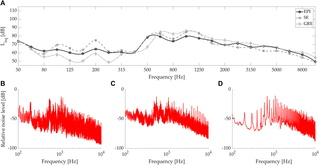
FIGURE 5. Noise level comparison between different MRI pulse sequences, at the isocenter of a 7 T scanner: (A) equivalent sound pressure level in one-third octave bands of EPI, SE, and GRE sequences. Noise level vs. frequency for (B) the SE sequence, (C) the EPI sequence, and (D) the GRE sequence.

3.2 Acoustic simulations in an empty cavity (configuration A)

To gain more insight from experimental results, numerical simulations were performed, as described in Section 2. Since it is impossible to reproduce in simulations the exact experimental boundary conditions, especially in terms of signal generation amplitudes and locations, the numerical study was limited to a modal analysis of the acoustic cavity. This allows to gain a better understanding of typical expected acoustic pressure spatial distributions, and to highlight recurring features, including amplitude maxima locations. An eigenmode analysis was thus first performed for configuration A. Two typical vibration mode types were mainly observed: longitudinal and azimuthal/radial modes. We choose to show, for illustration purposes, a single example of each aforementioned vibration mode, since the same conclusions can be drawn from analogous vibration modes at higher frequencies. Longitudinal-like modes showed constant normalized pressure (p) values for cross-sections in distinct z-coordinate values (Figure 6A), with a noticeable variation in pressure along the z-axis centreline (plotted for a 15 cm height in Figure 6B). Azimuthal or radial modes had opposing phases for the normalized pressure distribution for opposing x or y coordinates (Figure 6C) and a constant normalized pressure value along the cavity centreline (Figure 6D). The insets in Figures 6A, C show, for z between 150 mm and 200 mm, the absolute normalized pressure values (|p|), thus indicating that azimuthal or radial modes were concentrated on higher relative pressure values in the horizontal edges. Since the performed experimental measurements typically illustrated a small variation along the z-coordinate, this indicates that the MRI pulse sequences are mainly exciting azimuthal or radial vibration modes, probably as a result of the rotating operation of MRI scanners, which do not produce in-phase forces along the circumferential direction.

FIGURE 6

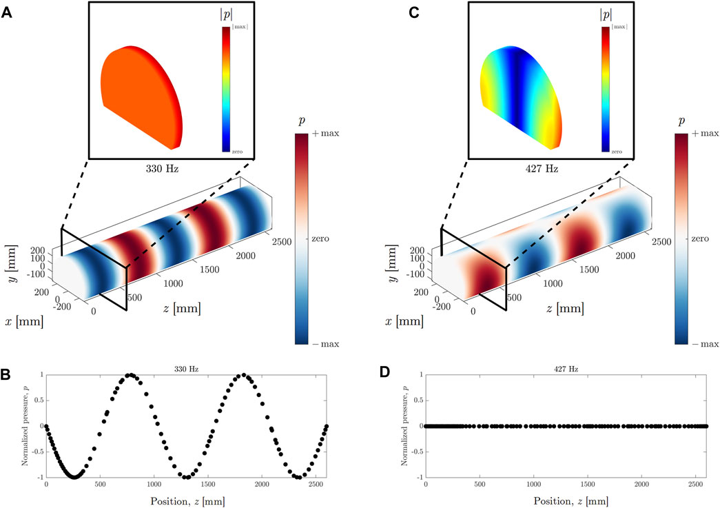
FIGURE 6. Typical simulated vibration modes. (A) Longitudinal-like vibration mode with a constant pressure distribution for each cross-section and (B) variable pressure along the bore centreline. (C) Bending-like (around the y direction) vibration mode with a varying pressure distribution for each cross-section (D) an almost constant pressure along the bore centreline. Insets correspond to z coordinates between 150 mm and 200 mm. Colour bars indicate either normalized (p) or absolute (|p|) pressures.

3.2 Noise measurements with a head phantom (configuration B)

The measurements in the presence of a phantom head show increased sound levels, due to strong reflections from the head towards the microphone positions. As shown in the Supplementary Figure SM5, results illustrate a very limited variability of the sound levels (L_eq) over the area around the ears (±5 cm from the isocentre along x). In the following, only the left ear data (M1) will be shown, given the symmetry of the measurement set-up and the scanner geometry. Figure 7 shows the details of the sound levels measured in the 7 T MRI scanner at the isocenter position (along y) of the left ear microphone for the EPI sequence. The frequency dependence of the noise levels was similar to that shown in Figure 4 (relative to the isocentre position) whereas absolute values were slightly different. The highest noise levels occurred in the 500–700 Hz band, with L_eq values up to 100 dB. Detailed waveform, spectrogram and narrow band power density spectral data are provided in the Supplementary Figure SM5.

FIGURE 7

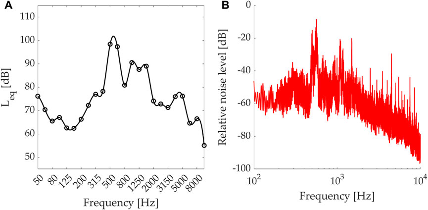
FIGURE 7. Noise measurements with a head phantom: (A) EPI sequence evaluated as equivalent sound pressure level in one-third octave bands, (B) Noise level vs. frequency at the left ear isocenter position (M1).

To further evaluate the impact of the type of MRI pulse sequences, the equivalent sound levels in third-octave bands were compared for the EPI and SE sequences. The values for a 7 T scanner (Figure 8B) are compared to those measured in a 3 T scanner (Figure 8A), for reference. The EPI and SE sequences displayed similar frequency profiles in both scanners, but the corresponding values were larger at 7 T. More specifically, noise levels at 7 T were higher in the mid frequency range, reaching values around 100 dB. A more detailed analysis is provided, based on the comparisons of the waveforms, spectrograms and narrow band power density spectra in the Supplementary Figures SM6, SM7.

FIGURE 8

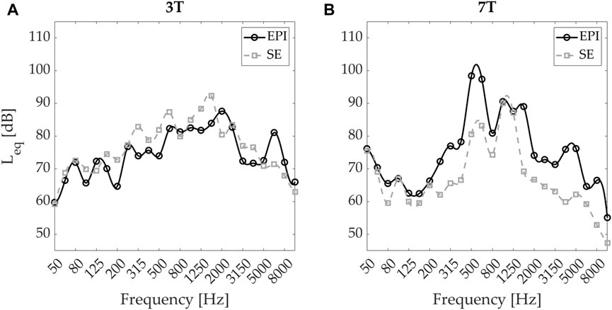
FIGURE 8. Noise Measurements with a head phantom: EPI and SE sequences evaluated as equivalent sound pressure level in one-third octave bands for (A) 3 T and (B) 7 T scanners at the left ear isocenter position.

Finally, a summary of results for the 7 T scanner is reported in Table 2, including all measurements in the two considered configurations, at different locations (isocentre, varying z-coordinates, and heights), for different signal sequences, and using different sound level descriptors: L_eq, L₉₀ (representing the levels that are exceeded for 90 percent of the time, usually used to quantify noise annoyance from industrial sources), L_mean (representing mean of the sound level), L_mode (representing the mode of the sound level).

TABLE 2

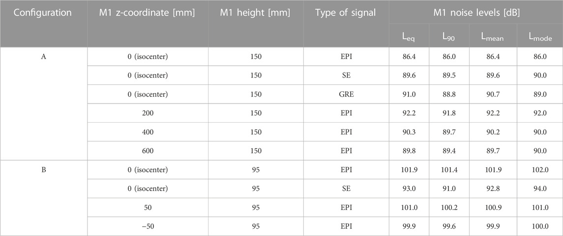
TABLE 2. Summary of M1 measured sound levels in the 7 T scanner, for different configurations (A or B), spatial locations, signal sequence type, and sound level descriptor.

3.3 Experimental-numerical comparison (configuration A)

Once again, these results were compared to those obtained from numerical simulations. In this case, the FE model included the scanner cavity and the phantom head, as shown in Figure 3C. Although the latter should be considered as composed as a soft, attenuative material, the approximation of using a perfectly rigid behaviour should yield very minor differences in the calculated acoustic field (especially in terms of the spatial field distribution) due to the large impedance mismatch with the surrounding fluid. Critical frequencies were considered, i.e., those displaying the most significant equivalent sound pressure levels in experimental measurements, such as 500 Hz and 632 Hz. Figures 9A, B display acoustic modes obtained for configurations A and B at 504 and 503 Hz, respectively, corresponding to azimuthal modes. Pressure concentrations occurred in the bottom and top parts of the cavity. In this case, the presence of the head phantom did not significantly modify the resonant frequency, but slightly modified the acoustic mode cross-section pressure distribution. In other words, a greater pressure was concentrated in the region around the head (see the insets representing z between 150 mm and 200 mm). Figures 9C, D display the results corresponding to 628 Hz and 625 Hz resonant frequencies. In this case, the azimuthal mode displayed pressure concentrations at the right and left parts of the cavity and this distribution was slightly affected by the presence of the head phantom. In both cases, the resonant frequencies were not significantly affected by the presence of the phantom volume. Although the cross-section pressure distribution was slightly modified by the presence of the phantom, the differences in the experimental values of equivalent sound pressure levels were better explained by the different positions of the microphones which shift from the centreline at z = 15 cm (configuration A) to off-centre (close to the phantom head ears) at z = 9 cm (configuration B). Nevertheless, the most significant acoustic modes might lead to a pressure concentration in either the vertical or horizontal directions, the latter being more troublesome due to their proximity to the ear region.

FIGURE 9

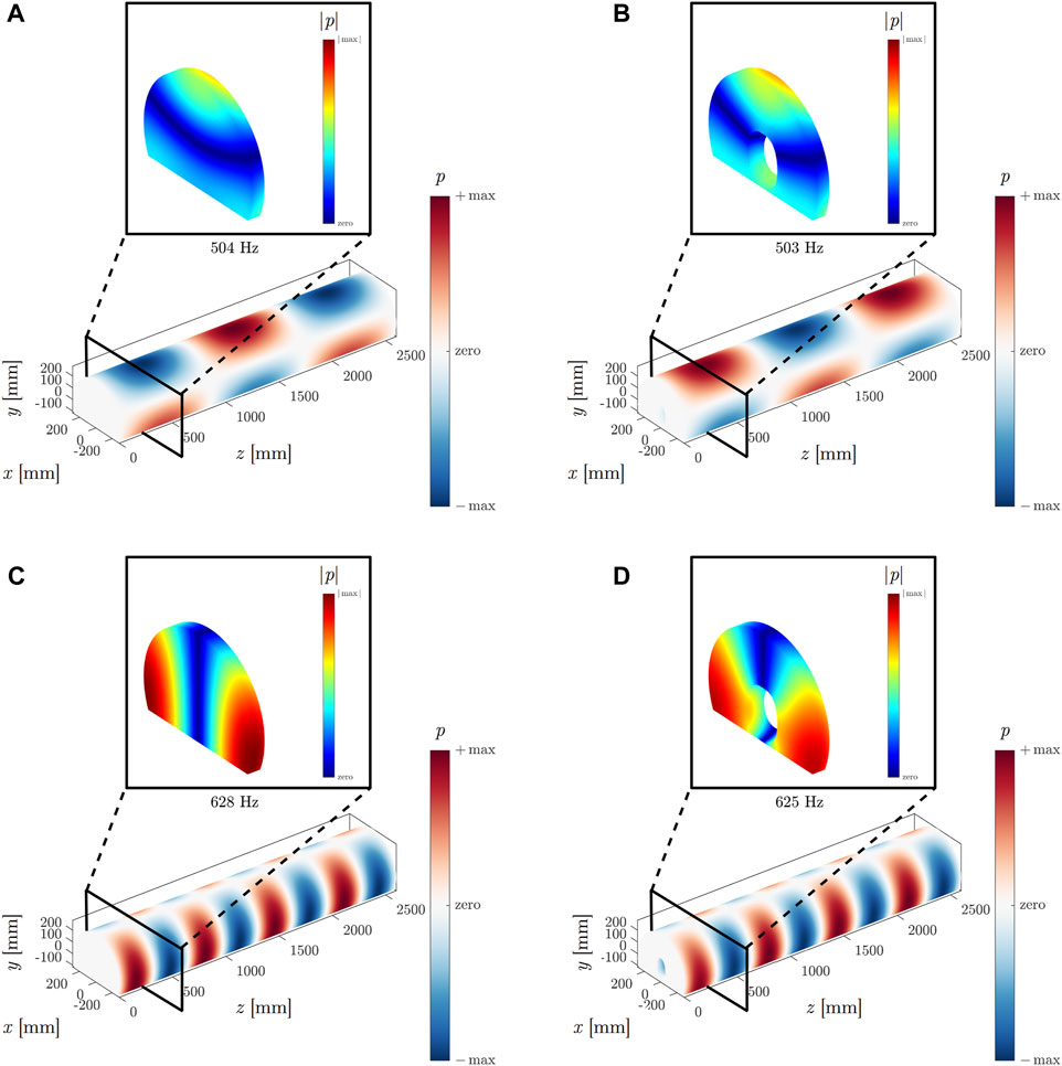
FIGURE 9. Simulated acoustic modes corresponding to frequencies with significant experimental equivalent sound pressure levels. Modes at around 500 Hz for (A) configuration A and (B) configuration B; Modes at around 630 Hz for (C) configuration A and (D) configuration (B). Insets show the sound levels in sections corresponding to z coordinates between 150 mm and 200 mm. Colour bars indicate either normalized (p) or absolute (|p|) pressures.

4 Conclusion

In conclusion, a detailed characterization and comparison of noise levels was performed in the audible frequency range in a 7 T MRI scanner located in the La Timone Hospital research centre, Marseille. The spatial variations were assessed along the central axis of the cavity and at different off-axis positions in the cavity, both with and without the presence of a phantom simulating the presence of a patient’s head. Both equivalent sound levels and peak levels were considered, to characterize exposure to mean and peak sound levels. Measurements were performed using various typical MRI pulse sequences which are known to provide the highest noise levels.

Our results indicate that sound levels are extremely high in this type of scanner, even more so than in widely used 1.5 T and 3 T scanners. Equivalent sound pressure levels were consistently above 70–80 dB (more than 20 dB above background noise), with maximum values around 90 dB in the frequency range around 500–3,000 Hz. Peak levels were consistently above 100 dB. These values were not available in the literature so far for 7 T scanners, due to their relatively recent introduction. The spatial variation of these levels was confined within the whole cavity region (in both axial and radial directions). The presence of a patient in the MRI scanner (simulated by a phantom head) was linked to increased noise levels (by 5–10 dB), as a result of strong reflections occurring between the head and the bore reflective walls and to the spatial variation of the acoustic modes. Numerical simulations confirmed experimental measurements and indicated that mostly azimuthal or radial modes were excited and contributed to the highest noise levels.

Overall, experimental and simulation results confirmed the critical level of noise within 7 T MRI scanners. At present, there is only one CE marked 7 T scanner available on the market, which is the one that we are considering in this study. Therefore, results from this study can be a reference study for further work on MRI technology in the Literature.

The measured noise levels further support the need of alternative solutions aiming at significantly reducing noise levels. Together with standard noise-abatement strategies, metamaterial layers can provide a workable solution for targeted sound absorption in specific frequency ranges. In particular, labyrinthine structures or space-coiling solutions can provide near-perfect absorption in the 500 Hz- 3 kHz range with a limited panel thickness (<1 cm) and unit cell sizes of few cm [42–44]. To extend the working frequency range, “rainbow” solutions can be adopted [45]. Work is in progress on this topic [46]. In any case, given the acoustic levels, optimal solutions can be obtained from the combination of existing strategies with metamaterial-based solutions which can address the most critical frequency ranges.

Acoustic measurements reported in the present study could be supplemented by surface vibration measurements using laser vibrometer. Such a combined analysis could provide information on the contribution of vibrations to the overall noise levels and indicate whether metamaterial solutions could also be used to reduce vibration transmission in the external panels of the MRI apparatus. The present experimental data, which comprises numerous time signals and their spatial variation in the MRI bore, can further be used to calibrate numerical models of the acoustic field generated therein as a function of the adopted signal sequences. Such a tool would be extremely useful for the assessment of different noise reduction strategies for MRI.

Data availability statement

The raw data supporting the conclusion of this article will be made available by the authors, without undue reservation.

Author contributions

LS: Formal Analysis, Investigation, Methodology, Writing–original draft, Writing–review and editing. VP: Investigation, Writing–original draft. CD: Writing–original draft, Investigation. MD: Investigation, Writing–original draft, Methodology. DB: Investigation, Writing–original draft. FN: Investigation, Formal Analysis, Writing–review and editing. MM: Writing–review and editing. NP: Writing–review and editing. FB: Conceptualization, Funding acquisition, Project administration, Supervision, Writing–original draft, Writing–review and editing.

Funding

The authors declare financial support was received for the research, authorship, and/or publication of this article. This work has been performed with the support of the European Commission under the FET Open “Boheme” Grant No. 863179 and FET Launchpad “Silence” Grant No. 101034788 as well as from the Excellence Initiative of Aix-Marseille University—A∗MIDEX, a French “Investissements d’Avenir” programme under the Multiwave chair of Medical Imaging.

Conflict of interest

Author CD was employed by the company Multiwave Technologies, Switzerland. Author MD was employed by Multiwave Imaging, France.

The remaining authors declare that the research was conducted in the absence of any commercial or financial relationships that could be construed as a potential conflict of interest.

Publisher’s note

All claims expressed in this article are solely those of the authors and do not necessarily represent those of their affiliated organizations, or those of the publisher, the editors and the reviewers. Any product that may be evaluated in this article, or claim that may be made by its manufacturer, is not guaranteed or endorsed by the publisher.

Supplementary material

The Supplementary Material for this article can be found online at: https://www.frontiersin.org/articles/10.3389/fphy.2023.1284659/full#supplementary-material

References

1. Mansfield P, Glover P, Bowtell R. Active acoustic screening: design principles for quiet gradient coils in MRI. Meas Sci Tech (1994) 5:1021–5. doi:10.1088/0957-0233/5/8/026

CrossRef Full Text | Google Scholar

2. Mansfield P, Glover PM, Beaumont J. Sound generation in gradient coil structures for MRI. Magn Reson Med (1998) 39:539–50. doi:10.1002/mrm.1910390406

PubMed Abstract | CrossRef Full Text | Google Scholar

3. McJury M, Shellock FG. Auditory noise associated with MR procedures: a review. J Magn Reson Imaging (2000) 12:37–45. doi:10.1002/1522-2586(200007)12:1<37::aid-jmri5>3.0.co;2-i

PubMed Abstract | CrossRef Full Text | Google Scholar

4. Bandettini PA, Jesmanowicz A, van Kylen J, Birn RM, Hyde JS. Functional MRI of brain activation induced by scanner acoustic noise. Magn Reson Med (1998) 39:410–6. doi:10.1002/mrm.1910390311

PubMed Abstract | CrossRef Full Text | Google Scholar

5. Cho ZH, Park SH, Kim JH, Chung S, Chung S, Chung J, et al. Analysis of acoustic noise in MRI. Magn Reson Imaging (1997) 15:815–22. doi:10.1016/s0730-725x(97)00090-8

PubMed Abstract | CrossRef Full Text | Google Scholar

6. Tomasi D, Caparelli EC, Chang L, Ernst T. fMRI-acoustic noise alters brain activation during working memory tasks. Neuroimage (2005) 27:377–86. doi:10.1016/j.neuroimage.2005.04.010

PubMed Abstract | CrossRef Full Text | Google Scholar

7. Counter SA, Olofsson A, Grahn HF, Borg E. MRI acoustic noise: sound pressure and frequency analysis. J Magn Reson Imaging (1997) 7:606–11. doi:10.1002/jmri.1880070327

PubMed Abstract | CrossRef Full Text | Google Scholar

8. Ravicz ME, Melcher JR, Kiang NYS. Acoustic noise during functional magnetic resonance imaging. J Acoust Soc America (2000) 108:1683–96. doi:10.1121/1.1310190

PubMed Abstract | CrossRef Full Text | Google Scholar

9. Price DL, de Wilde JP, Papadaki AM, Curran JS, Kitney RI. Investigation of acoustic noise on 15 MRI scanners from 0.2 T to 3 T. J Magn Reson Imaging (2001) 13:288–93. doi:10.1002/1522-2586(200102)13:2<288::aid-jmri1041>3.0.co;2-p

PubMed Abstract | CrossRef Full Text | Google Scholar

10. More SR, Lim TC, Li M, Holland CK, Boyce SE, Lee JH. Acoustic noise characteristics of a 4 Tesla MRI scanner. J Magn Reson Imaging (2006) 23:388–97. doi:10.1002/jmri.20526

PubMed Abstract | CrossRef Full Text | Google Scholar

11. McJury MJ. Acoustic noise and magnetic resonance imaging: a narrative/descriptive review. J Magn Reson Imaging (2022) 55:337–46. doi:10.1002/jmri.27525

PubMed Abstract | CrossRef Full Text | Google Scholar

12. Hedeen RA, Edelstein WA. Characterization and prediction of gradient acoustic noise in MR imagers. Magn Reson Med (1997) 37:7–10. doi:10.1002/mrm.1910370103

PubMed Abstract | CrossRef Full Text | Google Scholar

13. Nan J, Zong N, Chen Q, Zhang L, Zheng Q, Xia Y. A structure design method for reduction of MRI acoustic noise. Comput Math Methods Med (2017) 2017:6253428. doi:10.1155/2017/6253428

PubMed Abstract | CrossRef Full Text | Google Scholar

14. Edelstein WA, Hedeen RA, Mallozzi RP, El-Hamamsy SA, Ackermann RA, Havens TJ. Making MRI quieter. Magn Reson Imaging (2002) 20:155–63. doi:10.1016/s0730-725x(02)00475-7

PubMed Abstract | CrossRef Full Text | Google Scholar

15. Wyss M. Acoustic noise reduction in MRI based on pulse sequence optimization: analysis of sound characteristics and impact on sequence parameters. In: Proceedings of the Conference: ECR 2018; November 2018; Vienna, Austria (2018). doi:10.1594/ecr2018/C-2186

CrossRef Full Text | Google Scholar

16. Segbers M, Rizzo Sierra Cv., Duifhuis H, Hoogduin JM. Shaping and timing gradient pulses to reduce MRI acoustic noise. Magn Reson Med (2010) 64:546–53. doi:10.1002/mrm.22366

PubMed Abstract | CrossRef Full Text | Google Scholar

17. Yamashiro T, Morita K, Nakajima K. Evaluation of magnetic resonance imaging acoustic noise reduction technology by magnetic gradient waveform control. Magn Reson Imaging (2019) 63:170–7. doi:10.1016/j.mri.2019.08.015

PubMed Abstract | CrossRef Full Text | Google Scholar

18. Alibek S, Vogel M, Sun W, Winkler D, Baker CA, Burke M, et al. Acoustic noise reduction in MRI using Silent Scan: an initial experience. Diagn Interv Radiol (2014) 20:360–3. doi:10.5152/dir.2014.13458

PubMed Abstract | CrossRef Full Text | Google Scholar

19. Heismann B, Ott M, Grodzki D. Sequence-based acoustic noise reduction of clinical MRI scans. Magn Reson Med (2015) 73:1104–9. doi:10.1002/mrm.25229

PubMed Abstract | CrossRef Full Text | Google Scholar

20. Hall DA, Chambers J, Akeroyd MA, Foster JR, Coxon R, Palmer AR. Acoustic, psychophysical, and neuroimaging measurements of the effectiveness of active cancellation during auditory functional magnetic resonance imaging. J Acoust Soc America (2009) 125:347–59. doi:10.1121/1.3021437

PubMed Abstract | CrossRef Full Text | Google Scholar

21. Takkar MS, Kumar Sharma M, Pal R. A review on evolution of acoustic noise reduction in MRI. In: 2017 recent developments in control, automation and power engineering. Noida, India: RDCAPE 2017 (2017). p. 235–40.

CrossRef Full Text | Google Scholar

22. McJury M, Stewart RW, Crawford D, Toma E. The use of active noise control (ANC) to reduce acoustic noise generated during MRI scanning: some initial results. Magn Reson Imaging (1997) 15:319–22. doi:10.1016/s0730-725x(96)00337-2

PubMed Abstract | CrossRef Full Text | Google Scholar

23. Chen CK, Chiueh TD, Chen JH. Active cancellation system of acoustic noise in MR imaging. IEEE Trans Biomed Eng (1999) 46:186–91. doi:10.1109/10.740881

PubMed Abstract | CrossRef Full Text | Google Scholar

24. Li M, Lim TC, Lee JH. Simulation study on active noise control for a 4-T MRI scanner. Magn Resononance Imaging (2008) 26:393–400. doi:10.1016/j.mri.2007.08.003

PubMed Abstract | CrossRef Full Text | Google Scholar

25. Kanal E, Shellock FG. Policies, guidelines, and recommendations for MR imaging safety and patient management. J Magn Reson Imaging (1992) 2:247–8. doi:10.1002/jmri.1880020222

PubMed Abstract | CrossRef Full Text | Google Scholar

26. Craster Rv., Guenneau S. Acoustic metamaterials: negative refraction, imaging, lensing and cloaking. In: Acoustic metamaterials negative refraction, imaging, lensing and cloaking. Dordrecht: Springer (2013).

Google Scholar

27. Liu J, Guo H, Wang T. A review of acoustic metamaterials and phononic crystals. Crystals (Basel) (2020) 10(4):305. doi:10.3390/cryst10040305

CrossRef Full Text | Google Scholar

28. Assouar B, Oudich M, Zhou X. Acoustic metamaterials for sound mitigation. Comptes Rendus Physique (2016) 17:524–32. doi:10.1016/j.crhy.2016.02.002

CrossRef Full Text | Google Scholar

29. Arjunan A, Baroutaji A, Robinson J. Advances in acoustic metamaterials. Encyclopedia Smart Mater (2022) 3:1–10. doi:10.1016/b978-0-12-815732-9.00091-7

CrossRef Full Text | Google Scholar

30. . Oudich M, Zhou X, Badreddine Assouar M. General analytical approach for sound transmission loss analysis through a thick metamaterial plate. J Appl Phys (2014) 116:193509. doi:10.1063/1.4901997

CrossRef Full Text | Google Scholar

31. Xiao Y, Wen J, Wen X. Sound transmission loss of metamaterial-based thin plates with multiple subwavelength arrays of attached resonators. J Sound Vibrations (2012) 331:5408–23. doi:10.1016/j.jsv.2012.07.016

CrossRef Full Text | Google Scholar

32. Dal Poggetto VF, NicolaPugno JR de MFA, Arruda JRF. Bioinspired periodic panels optimized for acoustic insulation. Philosophical Trans R Soc A (2022) 380:2237. doi:10.1098/rsta.2021.0389

CrossRef Full Text | Google Scholar

33. Ghaffarivardavagh R, Nikolajczyk J, Anderson S, Zhang X. Ultra-open acoustic metamaterial silencer based on Fano-like interference. Phys Rev B (2019) 99:024302. doi:10.1103/physrevb.99.024302

CrossRef Full Text | Google Scholar

34. Sakhr J, Chronik BA. Parametric modeling of steady-state gradient coil vibration: resonance dynamics under variations in cylinder geometry. Magn Reson Imaging (2021) 82:91–103. doi:10.1016/j.mri.2021.06.007

PubMed Abstract | CrossRef Full Text | Google Scholar

35. Yao GZ, Mechefske CK, Rutt BK. Acoustic noise simulation and measurement of a gradient insert in a 4 T MRI. Appl Acoust (2005) 66:957–73. doi:10.1016/j.apacoust.2004.11.006

CrossRef Full Text | Google Scholar

36. Yao GZ, Mechefske CK, Rutt BK. Vibration analysis and measurement of a gradient coil insert in a 4 T MRI. J Sound Vibrations (2005) 285:743–58. doi:10.1016/j.jsv.2004.10.045

CrossRef Full Text | Google Scholar

37. Mechefske CK. MRI scanner vibration and acoustic noise. Proc ASME Int Des Eng Tech Conferences Comput Inf Eng Conf - DETC2005 (2008) 1:2575–85. doi:10.1115/DETC2005-84246

CrossRef Full Text | Google Scholar

38. Wu Z, Kim YC, Khoo MCK, Nayak KS. Evaluation of an independent linear model for acoustic noise on a conventional MRI scanner and implications for acoustic noise reduction. Magn Reson Med (2014) 71:1613–20. doi:10.1002/mrm.24798

PubMed Abstract | CrossRef Full Text | Google Scholar

39. NEMA. Standards publication MS 4-2010: acoustic noise measurement procedure for diagnosing magnetic resonance imaging devices (2010). Available at: https://www.nema.org/standards/view/Acoustic-Noise-Measurement-Procedure-for-Diagnostic-Magnetic-Resonance-Imaging-Devices.

Google Scholar

40. Fahy F, Gardonio P. Sound and structural vibration: radiation, transmission and response. Cambridge, Massachusetts: Academic Press (2007).

Google Scholar

41. Meeker T, Ah M. Guided wave propagation in elongated cylinders and plates. Phys Acoust (1964) 111–67. doi:10.1016/B978-1-4832-2857-0.50008-3

CrossRef Full Text | Google Scholar

42. Xie Y, Konneker A, Popa BI, Cummer SA. Tapered labyrinthine acoustic metamaterials for broadband impedance matching. Appl Phys Lett (2013) 103:201906. doi:10.1063/1.4831770

CrossRef Full Text | Google Scholar

43. Jiménez N, Huang W, Romero-García V, Pagneux V, Groby JP. Ultra-thin metamaterial for perfect and quasi-omnidirectional sound absorption. Appl Phys Lett (2016) 109:121902. doi:10.1063/1.4962328

CrossRef Full Text | Google Scholar

44. Boulvert J, Costa-Baptista J, Cavalieri T, Romero-García V, Gabard G, Fotsing ER, et al. Folded metaporous material for sub-wavelength and broadband perfect sound absorption. Appl Phys Lett (2020) 117:251902. doi:10.1063/5.0032809

CrossRef Full Text | Google Scholar

45. Jiménez N, Romero-García V, Pagneux V, Groby JP. Rainbow-trapping absorbers: broadband, perfect and asymmetric sound absorption by subwavelength panels for transmission problems. Scientific Rep (2017) 7:13595. doi:10.1038/s41598-017-13706-4

CrossRef Full Text | Google Scholar

46. Kamrul VH, Bettini L, Musso E, Nistri F, Piciucco D, Zemello M, et al. Proof of concept for a lightweight panel with enhanced sound absorption exploiting rainbow labyrinthine metamaterials (2021). Available at: https://arxiv.org/abs/2110.05026.

Google Scholar