Fractional derivative of demand and supply functions in the cobweb economics model and Markov process

This paper presents a more general cobweb model that incorporates the Hilfer fractional derivative in either the demand or supply function or Markov process. The main contributions of this study include deriving the analytical solution for the general model, analyzing the stability of the solution, introducing the equilibrium position using Mittag–Leffler functions, and providing detailed graphical illustrations to validate the effectiveness of the proposed model. The outcomes generalize some known results.

1 Introduction

In 1695, L’Hospital raised the question “dⁿy/dxⁿ if n = 1/2”? That is, “What if n is a fraction”? “This is an apparent paradox from which, one day, useful consequences will be drawn,” Leibniz replied [1]. Since then, the study of fractional derivatives gradually increased. Because the differential operator and the integral operator are inverse to each other, the fractional integral comes in. In short, the fractional integral is the extension of the ordinary integral, which changes the integral order into any real or complex order [2–4],. In the past decades, a large number of facts have proved that the fractional integral can be better prepared than the ordinary integral to simulate real-world phenomena, such as in physics [5–8] and in fluids mechanics[9,10], and more and more researchers like to use fractional integration for mathematical modeling [11–13, 14].

Fractional differential equations can simulate real-life situations better than ordinary differential equations [15]. There exist many different forms of fractional derivatives, namely, the Riemann–Liouville (R–L) fractional derivative[16,17], the Atangana–Baleanu fractional derivative[11,18,19], the Caputo–Fabrizio fractional derivative [20], the Caputo–Liouville (C–L) fractional derivative[16,17], the conformable fractional derivative[21,22], and so on. In the various types of fractional derivatives mentioned previously, the notation of the R–L fractional integral with order μ(0 < μ < 1) is fundamental [3,23–29].

Fractional derivatives play a significant role in economic modeling by providing a more accurate representation of real-world economic phenomena. Unlike traditional integer-order derivatives, fractional derivatives allow for the incorporation of memory effects and long-range dependencies, which are often observed in economic time series data [30–32]. Fractional derivatives capture these characteristics by accounting for the non-Markovian nature of economic processes, where past events and interactions can have a lasting impact on future outcomes. This is particularly relevant in financial markets, where the memory of past price movements and trading behaviors can influence future market dynamics [33–35]. One of the most significant models in economic dynamics, the cobweb economic model, defines the equilibrium price between supply and demand in a market over time [21,36,37]. In the case of pork, for instance, fewer people raised pigs last season due to some factor (such as the epidemic of disease or the increase in the price of pig feed), so this season’s pork production is bound to be low while the market demand remains the same. As a result, the market price of pork is bound to increase. After seeing increasing pork prices this season, more people decided to start raising pigs, which resulted in a substantially bigger supply of pork the following year. When supply outpaces demand and market demand stays the same, pork prices fall as a direct result. The farmers suffer from lower pork prices. As a result, fewer people raised pigs last season. Farmers are frequently powerless in the face of this, and the list goes on. Kaldor [38] examined this phenomenon and discovered that the prices of pork fluctuate like a spider’s web. He then provided a theoretical explanation of this economic event and used the term “cobweb theorem” to describe all economic occurrences that share this characteristic. The “cobweb theorem” was improved and expanded further in [39]. Later, Gandolfo [37] integrated the findings of earlier studies with his own to create a monograph that has since been the standard reference for scientists working on dynamical models.

Following closely in the footsteps of [40], this work deals with a more general cobweb economic model while taking the Hilfer fractional derivative into consideration. We provide the general model’s analytical solution and evaluate its stability. The present outcomes generalize the results of [41] and [40].

The remainder of this work is structured as follows: In Sections 2, 3, some fundamental concepts and theorems on the fractional derivative and cobweb theory are provided. The solution to this model is presented in Section 4, after which its stability is examined and the equilibrium point is calculated. One numerical example and comprehensive descriptions of graphical representations based on the concept are given in Section 5. Some findings are provided in Section 6.

2 Preliminaries on fractional derivatives

We recall the basic definitions and properties of the fractional integrals and the fractional derivatives which will be needed in the following.

Definition 2.1. [2,3,42,43] Let $\mu \in \mathbb{C},\mathfrak{R}(\mu )=[\mu ]+1$, $g:(a,b)\to \mathbb{R}$ be an integrable or differentiable function.

The right R–L fractional integral of order μ (0 < μ < 1) has the following form:

$\left({}^{RL}I_{a+}^{u}g\right)\left(x\right)=\frac{1}{\mathrm{\Gamma }\left(u\right)}{\int }_a^x{\left(x-t\right)}^{u-1}g\left(t\right)dt.(1)$

The right R–L fractional derivative of order μ $(\mu \in \mathbb{C})$ has the following form:

$\left({}^{RL}D_{a+}^{u}g\right)\left(x\right)=\left(D^n{D}^{\mu -n}g\right)\left(x\right)={\left(\frac{d}{dx}\right)}^n\left(I_{a+}^{n-u}g\right)\left(x\right)=\left\{\begin{array}{cc}\hfill & \frac{1}{\mathrm{\Gamma }\left(n-u\right)}{\left(\frac{d}{dx}\right)}^n{\int }_a^x{\left(x-t\right)}^{n-u-1}g\left(t\right)dt,\hfill \\ \hfill & if\mu \notin \mathbb{N},n=\mathfrak{R}\left(u\right),\hfill \\ \hfill & g^{\left(n\right)}\left(x\right),if\mu =n\in \mathbb{N}.\hfill \end{array}\right.(2)$

The right C–L fractional derivative of order μ $(\mu \in \mathbb{C})$ takes the following form:

$\left({}^{CL}D_{a+}^{u}g\right)\left(x\right)=\left(D^{\mu -n}{D}^{n}g\right)\left(x\right)=\left(I_{a+}^{n-u}{g}^{\left(n\right)}\right)\left(x\right)=\left\{\begin{array}{cc}\hfill & \frac{1}{\mathrm{\Gamma }\left(n-u\right)}{\int }_a^x{\left(x-t\right)}^{n-u-1}{g}^{\left(n\right)}\left(t\right)dt,\hfill \\ \hfill & if\mu \notin \mathbb{N},n=\mathfrak{R}\left(u\right),\hfill \\ \hfill & g^{\left(n\right)}\left(x\right),if\mu =n\in \mathbb{N}.\hfill \end{array}\right)(3)$

where [μ] denotes the largest integer that do not exceed μ, so $\mathfrak{R}(\mu )=[\mu ]+1$ means the smallest integer greater than μ, and Γ(⋅) denotes the Gamma function.

Definition 2.2. [2,3,42,43] Let $\mu \in \mathbb{C}$, $\mathfrak{R}(\mu )>0$, $g:(a,b)\to \mathbb{R}$ be an integrable or differentiable function.

The left R–L fractional integral of order μ (0 < μ < 1) has the following form:

$\left({}^{RL}I_{b-}^{u}g\right)\left(x\right)=\frac{1}{\mathrm{\Gamma }\left(u\right)}{\int }_x^b{\left(t-x\right)}^{u-1}g\left(t\right)dt.(4)$

The left R–L fractional derivative of order μ $(\mu \in \mathbb{C})$ has the following form:

$\left({}^{RL}D_{b-}^{u}g\right)\left(x\right)={\left(-\frac{d}{dx}\right)}^n\left(I_{b-}^{n-u}g\right)\left(x\right)=\left\{\begin{array}{cc}\hfill & \frac{1}{\mathrm{\Gamma }\left(n-u\right)}{\left(-1\right)}^n{\left(\frac{d}{dx}\right)}^n{\int }_x^b{\left(t-x\right)}^{n-u-1}g\left(t\right)dt,\hfill \\ \hfill & if\mu \notin \mathbb{N},n=\mathfrak{R}\left(\mu \right),\hfill \\ \hfill & g^{\left(n\right)}\left(x\right),if\mu =n\in \mathbb{N}.\hfill \end{array}\right.(5)$

The left C–L fractional derivative of order μ $(\mu \in \mathbb{C})$ takes the following form:

$\left({}^{CL}D_{b-}^{u}g\right)\left(x\right)=\left(I_{b-}^{n-u}{\left(-1\right)}^n{g}^{\left(n\right)}\right)\left(x\right)=\left\{\begin{array}{cc}\hfill & \frac{1}{\mathrm{\Gamma }\left(n-u\right)}{\int }_x^b{\left(t-x\right)}^{n-u-1}{\left(-1\right)}^n{g}^{\left(n\right)}\left(t\right)dt,\hfill \\ \hfill & if\mu \notin \mathbb{N},n=\mathfrak{R}\left(\mu \right),\hfill \\ \hfill & g^{\left(n\right)}\left(x\right),if\mu =n\in \mathbb{N}.\hfill \end{array}\right.(6)$

The generalized R–L fractional derivative, also called the Hilfer fractional derivative [1,40], is defined as follows:

Definition 2.3. [1,15,44] $D_{a+}^{\mu ,\nu }$ and $D_{a-}^{\mu ,\nu }$ of order μ (0 < μ < 1) and type ν (0 ≤ ν ≤ 1) with respect to x defined by, respectively,

$\left(D_{a+}^{\mu ,\nu }g\right)\left(x\right)=\left({}^{RL}I_{a+}^{\nu \left(1-\mu \right)}\frac{d}{dx}\left({}^{RL}I_{a+}^{\left(1-\nu \right)\left(1-\mu \right)}g\right)\right)\left(x\right)=\left({}^{RL}I_{a+}^{\nu \left(1-\mu \right)}\left(D_{a+}^{\mu +\nu -\mu \nu }g\right)\right)\left(x\right)(7)$

and

$\left(D_{a-}^{\mu ,\nu }g\right)\left(x\right)=\left(-{}^{RL}I_{a-}^{\nu \left(1-\mu \right)}\frac{d}{dx}\left({}^{RL}I_{a-}^{\left(1-\nu \right)\left(1-\mu \right)}g\right)\right)\left(x\right)=\left(-{}^{RL}I_{a-}^{\nu \left(1-\mu \right)}\left(D_{a-}^{\mu +\nu -\mu \nu }g\right)\right)\left(x\right)(8)$

are called the right-sided and left-sided Hilfer fractional derivatives, where $({}^{RL}I_{a\pm }^{(1-\nu )(1-\mu )}g)(x)$ is the R–L fractional integral of function g(x) of the order (1 − ν)(1 − μ), given by (1) and (4).

From Definition 2.3, we can find that if ν = 0,

$\left(D_{a\pm }^{\mu ,0}g\right)(x)=\left(\pm {}^{RL}I_{a\pm }^0\frac{d}{dx}\left({}^{RL}I_{a\pm }^{(1-\mu )}g\right)\right)(x)=\pm \frac{d}{dx}\left({}^{RL}I_{a\pm }^{(1-\mu )}g\right)(x),$

and it turns into the R–L fractional derivative of order μ [(2) and (5)].

Moreover, if ν = 1,

$\left(D_{a\pm }^{\mu ,1}g\right)(x)=\left(\pm {}^{RL}I_{a\pm }^{(1-\mu )}\frac{d}{dx}\left({}^{RL}I_{a\pm }^{0}g\right)\right)(x)=\pm \left({}^{RL}I_{a\pm }^{(1-\mu )}{g}^{\prime }\right)(x),$

and it turns into the C–L fractional derivative of order μ [ (3) and (6)]. More applications of $D_{a\pm }^{\mu ,\nu }$ could be found in the work of Hilfer [45].

In order to obtain the analytical solution of the model with the Hilfer fractional derivative, we use the Mittag–Leffler function given by Definition 2.4.

Definition 2.4. [3,40,42,46] The Mittag–Leffler functions E_α(z) and E_α,β(z) are given as follows:

$E_{\alpha }\left(z\right)={\displaystyle \sum _{k=0}^{\infty }}\frac{z^k}{\mathrm{\Gamma }\left(\alpha k+1\right)}{E}_{\alpha ,\beta }\left(z\right)={\displaystyle \sum _{k=0}^{\infty }}\frac{z^k}{\mathrm{\Gamma }\left(\alpha k+\beta \right)}\left(z,\alpha ,\beta \in \mathbb{C};\mathfrak{R}\left(\alpha \right)>0\right).(9)$

Hence, $E_{\alpha ,1}(z)=E_{\alpha }(z),E_{\mathrm{1,1}}(z)=\sum _{k=0}^{\infty }\frac{z^k}{\mathrm{\Gamma }(k+1)}=e^z$, and furthermore,

$\begin{array}{ll}\hfill E_1(z)& =e^z,E_2(z^2)=\cosh z,E_2(-z^2)=\cos z,\hfill \\ \hfill E_{\mathrm{0,1}}(z)& =\frac{1}{1-z},E_{\mathrm{1,2}}(z)=\frac{e^z-1}{z},E_{\mathrm{2,1}}(z)=\cosh (\sqrt{z}),\hfill \\ \hfill E_{\mathrm{2,2}}(z)& =\frac{\sinh z}{z}.\hfill \end{array}$

Next, we present some properties of Mittag–Leffler functions proved in some existing literature.

Lemma 2.1. [47] Let $0<\alpha <2,\frac{\pi \alpha }{2}<\theta <\min \{\pi ,\alpha \pi \}$, ∀ h ∈ Z⁺ (Z is the integer set); there exists

$E_{\alpha }(z)=-{\displaystyle \sum _{k=1}^h}\frac{z^{-k}}{\mathrm{\Gamma }(1-\alpha k)}+O(|z{|}^{-1-h})\left(|z|\to \infty ,\theta \le |\arg (z)|\le \pi \right).$

Lemma 2.2. [48] If 0 < α, β < 2, αβ < 2 and $\frac{\pi \alpha \beta }{2}<\theta <\min \{\pi ,\alpha \beta \pi \}$, then ∀ h ∈ Z⁺,

$E_{\alpha ,\beta }(z)=-{\displaystyle \sum _{k=1}^h}\frac{z^{-k}}{\mathrm{\Gamma }(\beta -\alpha k)}+O(|z{|}^{-1-h})\left(|z|\to \infty ,\theta \le |\arg (z)|\le \pi \right).$

Lemma 2.3. [40] When z → ∞, then the results of Lemma 2.1 and Lemma 2.2 reduce to 0; that is,

${\displaystyle \underset{z\to \infty }{\lim }}{E}_{\alpha }(-z)={\displaystyle \underset{z\to \infty }{\lim }}\left(-{\displaystyle \sum _{k=1}^h}\frac{{(-z)}^{-k}}{\mathrm{\Gamma }(1-\alpha k)}+O(|-z{|}^{-1-h})\right)\to 0$

and

${\displaystyle \underset{z\to \infty }{\lim }}{E}_{\alpha ,\beta }(-z)={\displaystyle \underset{z\to \infty }{\lim }}\left(-{\displaystyle \sum _{k=1}^h}\frac{{(-z)}^{-k}}{\mathrm{\Gamma }(\beta -\alpha k)}+O(|-z{|}^{-1-h})\right)\to 0,$

Lemma 2.4. [1,3,44] The Laplace transform of the Hilfer fractional derivative of g(t) satisfies

$\mathcal{L}\left\{\left(D_{0+}^{\mu ,\nu }g\right)\left(t\right):s\right\}=s^{\mu }\mathcal{L}\left\{g\left(t\right):s\right\}-s^{\nu \left(\mu -1\right)}\left({}^{RL}I_{0+}^{\left(1-\nu \right)\left(1-\mu \right)}g\right)\left(0+\right),(10)$

where $\mathcal{L}$ of Laplace transform is

$\mathcal{L}\{g(t):s\}≔{\int }_0^{\infty }{e}^{-st}g(t)dt≕G(s)$

and

$\left({}^{RL}I_{0+}^{(1-\nu )(1-\mu )}g\right)(0+)≔{\left.\left({}^{RL}I_{0+}^{(1-\nu )(1-\mu )}g\right)(t)\right|}_{t\to 0+}$

and

$\mathcal{L}\left\{t^{\beta -1}{E}_{\alpha ,\beta }\left(\lambda t^{\alpha }\right):s\right\}=\frac{s^{\alpha -\beta }}{s^{\alpha }-\lambda },(11)$

$\mathcal{L}\left\{1-E_{\alpha }\left(\lambda t^{\alpha }\right):s\right\}=\frac{-\lambda }{s\left(s^{\alpha }-\lambda \right)},(12)$

with $\mathfrak{R}(s)>0,\mathfrak{R}(\alpha )>0,\lambda \in \mathbb{C}$ and |λs^−α| < 1.

3 Cobweb economic model

In this section, we give some definitions and theorems of cobweb models.

Gandolfo [37] studied the cobweb models with (13) and (14) (see also in [41,49]).

$\left\{\begin{array}{cc}\hfill D\left(t\right)& =a+bp\left(t+1\right),\text{demand}\hfill \\ \hfill S\left(t\right)& =a_1+b_{1}p\left(t\right),\text{supply}\hfill \\ \hfill D\left(t\right)& =S\left(t\right).\text{market\hspace{0.17em}clearing}\hfill \end{array}\right.(13)$

where p(t) is the market price at time t and p (t + 1) is the market price at time t + 1. D(t), S(t) is the market demand and market supply at time t, respectively.

$\left\{\begin{array}{cc}\hfill D\left(t\right)& =a+bp\left(t\right),\text{demand}\hfill \\ \hfill S\left(t\right)& =a_1+b_1\left(p\left(t\right)+c{p}^{\prime }\left(t\right)\right),\text{supply}\hfill \\ \hfill D\left(t\right)& =S\left(t\right),\text{market\hspace{0.17em}clearing}\hfill \end{array}\right.(14)$

where p(t) + cp′t) denotes the expected price at time t; that is, the price that producers anticipate will remain stable after output is realized at the time of production is initiated. The commonly used form of p(t) + cp′t) is p(t) + c (p (t + 1) − p(t)) [49], and c > 0 measures the consumer’s price sensitivity to the price difference. The implications behind (13) and (14) are described as follows. In the demand function, a is the market potential and b is the consumer’s price sensitivity coefficient. The larger b means the more sensitive consumers, and a small piece price drop may attract a large portion of consumers to make the consumption. To make the analysis realistic, we assume that a > 0, b < 0. In reality, as prices increase, supply increases throughout the supply curve, and as prices decline, supply decreases along the supply curve, so we set a₁ > 0, b₁ > 0 in the supply function to make the analysis realistic. Both functions (13) and (14) are linear; the output from the beginning of the period appears at the conclusion of each period, and the market sets its price. When production manifests after a period, the price used to determine it is undoubtedly the price from the previous period. Supply responds to price with a one-period lag, whereas demand is dependent on the current price. In each period, the price is set by the market so that demand consumes exactly the amount that is supplied, leaving no producer with unsold product and no consumer with unmet need (i.e., D(t) = S(t)).

Based on (13), Gandolfo [37] improved the model by taking the following form:

$\left\{\begin{array}{cc}\hfill D\left(t\right)& =a+b\left(p\left(t\right)+p^{\prime }\left(t\right)\right),\hfill \\ \hfill S\left(t\right)& =a_1+b_{1}p\left(t\right),\hfill \\ \hfill D\left(t\right)& =S\left(t\right).\hfill \end{array}\right.(15)$

Lemma 3.1. [40,41]The solutions of (13), (14), and (15) are

$\begin{array}{ccc}\hfill p\left(t\right)& =\hfill & \left(p_0-p_e\right){\left(\frac{b_1}{b}\right)}^t+p_e;\hfill \\ \hfill p\left(t\right)& =\hfill & \left(p_0-p_e\right)e^{\left(\frac{b-b_1}{b_{1}c}\right)t}+p_e;\hfill \\ \hfill p\left(t\right)& =\hfill & \left(p_0-p_e\right)e^{\left(\frac{b_1-b}{b}\right)t}+p_e,\hfill \end{array}$

respectively, where $p_0\in \mathbb{R}$ is the initial price of p(t) and $p_e=\frac{a_1-a}{b-b_1}$ is called the equilibrium value.

It can be verified that only when $|\frac{b_1}{b}|<1,|\frac{b-b_1}{b_{1}c}|<1,|\frac{b_1-b}{b}|<1$, the solutions of (13), (14), and (15) converge to the equilibrium value p_e. Since b < 0 and b₁ > 0, they are divergent if $\frac{b_1}{b}<-1$; steady if $\frac{b_1}{b}=-1$; and damped if $-1<\frac{b_1}{b}\le 0$. Figure 1 plots the solutions when $-1<\frac{b_1}{b}\le 0,-1<\frac{b-b_1}{b_{1}c}\le 0$ and $-1<\frac{b_1-b}{b}\le 0$.

FIGURE 1

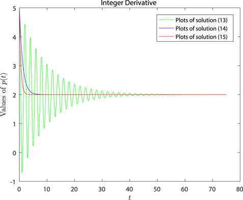
FIGURE 1. Basic cobweb model with an integer derivative.

Chen et al. [41] considered the basic cobweb model [(14) and (15)] with the C–L fractional derivative as follows:

$\begin{array}{lll}\hfill & \left\{\begin{array}{cc}\hfill D\left(t\right)& =a+bp\left(t\right),\hfill \\ \hfill S\left(t\right)& =a_1+b_1\left(p\left(t\right)+c{\cdot }^{CL}{D}_{0+}^{\mu }p\left(t\right)\right),\hfill \\ \hfill D\left(t\right)& =S\left(t\right).\hfill \end{array}\right.\hfill & \hfill \left\{\begin{array}{cc}\hfill D\left(t\right)& =a+b\left(p\left(t\right){+}^{CL}{D}_{0+}^{\mu }p\left(t\right)\right),\hfill \\ \hfill S\left(t\right)& =a_1+b_{1}p\left(t\right),\hfill \\ \hfill D\left(t\right)& =S\left(t\right).\hfill \end{array}\right.\end{array}(16)$

where $0<\mu \le 1,a,b,a_1,b_1,c\in \mathbb{R},b\ne 0,b\ne b_1$ and ${}^{CL}D_{0+}^{\mu }p(t)$ are given in (3).

Chen et al. [41] obtained the main results of (16) and studied the stability of the solution. Srivastava et al. [40] generalized Chen et al.’s [41] conclusion, and they considered the fractional derivatives as follows:

$\begin{array}{lll}\hfill & \left\{\begin{array}{cc}\hfill D\left(t\right)& =a+b\left(p\left(t\right)+D_{0+}^{\mu ,\nu }p\left(t\right)\right),\hfill \\ \hfill S\left(t\right)& =a_1+b_{1}p\left(t\right),\hfill \\ \hfill D\left(t\right)& =S\left(t\right).\hfill \end{array}\right.\hfill & \hfill \left\{\begin{array}{cc}\hfill D\left(t\right)& =a+bp\left(t\right),\hfill \\ \hfill S\left(t\right)& =a_1+b_1\left(p\left(t\right)+c\cdot D_{0+}^{\mu ,\nu }p\left(t\right)\right),\hfill \\ \hfill D\left(t\right)& =S\left(t\right).\hfill \end{array}\right.\end{array}(17)$

where $D_{0+}^{\mu ,\nu }p(t)$ is the Hilfer fractional derivative given by (7), $a,b,a_1,b_1,c\in \mathbb{R},b\ne 0,b\ne b_1,0<\mu \le 1$, and 0 ≤ ν ≤ 1.

In this paper, we consider the cobweb model (17) with the Hilfer fractional derivative $D_{a+}^{\mu ,\nu }$ in the supply function and in the demand function together as the following form:

$\left\{\begin{array}{cc}\hfill D\left(t\right)& =a+b\left(p\left(t\right)+\theta \cdot D_{0+}^{\mu ,\nu }p\left(t\right)\right),\hfill \\ \hfill S\left(t\right)& =a_1+b_1\left(p\left(t\right)+{\theta }_1\cdot D_{0+}^{\mu ,\nu }p\left(t\right)\right),\hfill \\ \hfill D\left(t\right)& =S\left(t\right).\hfill \end{array}\right.,(18)$

where $D_{0+}^{\mu ,\nu }p(t)$ is the Hilfer fractional derivative given by (7). We set $a>0,b<0,a_1>0,b_1>0;\theta ,{\theta }_1\in \mathbb{R}$; 0 < μ ≤ 1; and 0 ≤ ν ≤ 1.

Our model generalizes some known models such as those in [41] and [40]. Specifically, when θ = 0, ν = 1, (18) reduces to the first half of (16); when θ₁ = 0, ν = 1, (18) reduces to the last half of (16); when θ₁ = 0, θ = 1, (18) turns into the first half of (17); and when θ = 0, (18) turns into the last half of (17).

4 Cobweb model with the Hilfer fractional derivative

In this section, we calculate the solution of the cobweb model (18) and study the stability of the solution.

Theorem 4.1. The following equation solves the cobweb model (18):

$p\left(t\right)=C_0{t}^{\gamma -1}{E}_{\mu ,\gamma }\left(\lambda t^{\mu }\right)-\frac{\xi }{\lambda }+\frac{\xi }{\lambda }{E}_{\mu }\left(\lambda t^{\mu }\right),(19)$

where

$\gamma =\mu +\nu -\mu \nu ,\lambda =\frac{b_1-b}{b\theta -b_1{\theta }_1},\xi =\frac{a_1-a}{b\theta -b_1{\theta }_1},$

and $C_0\in \mathbb{R}$ satisfies

$C_0=\left({}^{RL}I_{0+}^{\left(1-\nu \right)\left(1-\mu \right)}p\right)\left(0+\right)={\left.\left({}^{RL}I_{0+}^{\left(1-\nu \right)\left(1-\mu \right)}p\right)\left(t\right)\right|}_{t\to 0+}.$

Proof: By simplifying the model (18), we obtain

$a+b\left(p\left(t\right)+\theta \cdot \left(D_{0+}^{\mu ,\nu }p\right)\left(t\right)\right)=a_1+b_1\left(p\left(t\right)+{\theta }_1\cdot \left(D_{0+}^{\mu ,\nu }p\right)\left(t\right)\right),$

so

$\left(b\theta -b_1{\theta }_1\right)\left(D_{0+}^{\mu ,\nu }p\right)\left(t\right)=\left(a_1-a\right)+\left(b_1-b\right)p\left(t\right).$

If bθ − b₁θ₁ ≠ 0, we have

$\left(D_{0+}^{\mu ,\nu }p\right)\left(t\right)=\frac{a_1-a}{b\theta -b_1{\theta }_1}+\frac{b_1-b}{b\theta -b_1{\theta }_1}p\left(t\right).$

Letting $\xi =\frac{a_1-a}{b\theta -b_1{\theta }_1}$ and $\lambda =\frac{b_1-b}{b\theta -b_1{\theta }_1}$, we have

$\left(D_{0+}^{\mu ,\nu }p\right)\left(t\right)=\lambda p\left(t\right)+\xi .(20)$

Taking the Laplace transform of (20), we have

$\mathcal{L}\left\{D_{0+}^{\mu ,\nu }\left(p\right)\left(t\right):s\right\}=\lambda \mathcal{L}\left\{p\left(t\right):s\right\}+\mathcal{L}\left\{\xi :s\right\}.$

Using the Laplace transform formula (10) for the Hilfer fractional derivative, we have

$s^{\mu }\mathcal{L}\left\{p\left(t\right):s\right\}-s^{\nu \left(\mu -1\right)}\left({}^{RL}I_{0+}^{\left(1-\nu \right)\left(1-\mu \right)}p\right)\left(0+\right)=\lambda \mathcal{L}\left\{p\left(t\right):s\right\}+\frac{\xi }{s}.$

Merging items of the same type, we have

$s^{\mu }\mathcal{L}\left\{p\left(t\right):s\right\}-\lambda \mathcal{L}\left\{p\left(t\right):s\right\}=s^{\nu \left(\mu -1\right)}\left({}^{RL}I_{0+}^{\left(1-\nu \right)\left(1-\mu \right)}p\right)\left(0+\right)+\frac{\xi }{s},$

and then,

$\mathcal{L}\left\{p\left(t\right):s\right\}=\frac{s^{\nu \left(\mu -1\right)}\left({}^{RL}I_{0+}^{\left(1-\nu \right)\left(1-\mu \right)}p\right)\left(0+\right)}{s^{\mu }-\lambda }+\frac{\xi }{s\left(s^{\mu }-\lambda \right)}.$

Setting $({}^{RL}I_{0+}^{(1-\nu )(1-\mu )}p)(0+)=C_0$, we have

$\mathcal{L}\left\{p\left(t\right):s\right\}=\frac{C_0\cdot s^{\nu \left(\mu -1\right)}}{s^{\mu }-\lambda }+\frac{\xi }{s\left(s^{\mu }-\lambda \right)}.$

Using the application of Eqs (11), (12), we have

$\frac{\xi }{s\left(s^{\mu }-\lambda \right)}=\frac{\xi }{-\lambda }\cdot \frac{-\lambda }{s\left(s^{\mu }-\lambda \right)}=-\frac{\xi }{\lambda }\cdot L\left\{1-E_{\mu }\left(\lambda t^u\right):s\right\}$

and

$\frac{s^{\nu \left(\mu -1\right)}}{s^{\mu }-\lambda }=\frac{s^{\mu -\gamma }}{s^{\mu }-\lambda }=L\left\{t^{\gamma -1}{E}_{\mu ,\gamma }\left(\lambda t^u\right):s\right\},$

where μ − γ = ν(μ − 1), so γ = μ + ν − μν, and we arrive at

$\mathcal{L}\left\{p\left(t\right):s\right\}=C_0\mathcal{L}\left\{t^{\gamma -1}{E}_{\mu ,\gamma }\left(\lambda t^u\right):s\right\}-\frac{\xi }{\lambda }\mathcal{L}\left\{1-E_{\mu }\left(\lambda t^u\right):s\right\}.(21)$

Finally, by employing the inverse Laplace transform of (21), it can be found that

$p\left(t\right)=C_0{t}^{\gamma -1}{E}_{\mu ,\gamma }\left(\lambda t^u\right)-\frac{\xi }{\lambda }+\frac{\xi }{\lambda }{E}_{\mu }\left(\lambda t^u\right),$

where γ = μ + ν − μν.

Theorem 4.2. When θ > 0, θ₁ > 0, the solution of (18) converges to the equilibrium value p_e, which satisfies

$p_e=\frac{a_1-a}{b-b_1}.$

Proof: In model (18), we assume a > 0, b < 0, a₁ > 0, b₁ > 0 to make our analysis in line with reality. From Theorem 4.1, we know that $\lambda =\frac{b_1-b}{b\theta -b_1{\theta }_1}$ and $\xi =\frac{a_1-a}{b\theta -b_1{\theta }_1}$.

When θ > 0, θ₁ > 0, then λ < 0. Since 0 < μ ≤ 1, λt^μ → −∞ (t → ∞), and in light of Lemma 2.3, when λt^u → −∞, we have

$\underset{t\to \infty }{\lim }{E}_{\mu }\left(\lambda t^{\mu }\right)=0.$

Hence

$\underset{t\to \infty }{\lim }p\left(t\right)=\underset{t\to \infty }{\lim }\left(C_0{t}^{\gamma -1}{E}_{\mu ,\gamma }\left(\lambda t^{\mu }\right)-\frac{\xi }{\lambda }\right).(22)$

Since γ = −(1 − μ)(1 − ν) + 1, γ ∈ (0, 1], and we make the analysis from two aspects:

i) When γ = 1, from (22), we have

$\underset{t\to \infty }{\lim }{C}_0{t}^0{E}_{\mu ,1}(\lambda t^{\mu })=\underset{t\to \infty }{\lim }{C}_0{E}_{\mu }(\lambda t^{\mu })=0.$

Hence, we obtain

$\underset{t\to \infty }{\lim }p(t)=-\frac{\xi }{\lambda }.$

ii) When 0 < γ < 1, t^γ−1 → 0 (t → ∞) and λt^μ → −∞ (t → ∞). In light of Lemma 2.3,

$\underset{t\to \infty }{\lim }{C}_0{t}^{\gamma -1}{E}_{\mu ,\gamma }(\lambda t^{\mu })\to 0.$

Hence, we obtain

$\underset{t\to \infty }{\lim }p(t)=-\frac{\xi }{\lambda }.$

Overall,

$\underset{t\to \infty }{\lim }p(t)=-\frac{\xi }{\lambda }=\frac{a_1-a}{b-b_1}=p_e,$

which completes the proof of Theorem 2.2.

The stability conditions θ > 0 and θ₁ > 0 play a crucial role in determining the stability of the equilibrium price (p_e) in a market. We provide the explanation as follows.

First, the condition θ > 0 is related to the price elasticity of demand. It indicates that the demand function is negatively sloped, meaning that as the price increases, the quantity demanded decreases. This condition ensures that the market is responsive to changes in price, and it reflects the typical behavior observed in most markets. When θ > 0, it implies that an increase in price will lead to a decrease in demand, which helps maintain stability in the market. If θ were to be negative, it would imply an upward-sloping demand curve, which could lead to instability and oscillations in the market. Second, the condition θ₁ > 0 is associated with the price elasticity of supply. It signifies that the supply function is positively sloped, indicating that as the price increases, the quantity supplied also increases. This condition ensures that suppliers are willing to increase their production in response to higher prices, maintaining stability in the market. If θ₁ were negative, it would imply a downward-sloping supply curve, which could lead to instability and fluctuations in the market.

In terms of market stability, when both θ > 0 and θ₁ > 0 hold, the market tends to reach a stable equilibrium price where demand and supply are balanced. In this scenario, any temporary imbalances between demand and supply will be corrected through price adjustments, ensuring market stability.

To compare the difference between integer derivatives and fractional derivatives, we consider the basic cobweb model with integer derivatives in supply and demand function together as the following form:

$\left\{\begin{array}{cc}\hfill D\left(t\right)& =a+b\left(p\left(t\right)+\theta \cdot p^{\prime }\left(t\right)\right),\hfill \\ \hfill S\left(t\right)& =a_1+b_1\left(p\left(t\right)+{\theta }_1\cdot p^{\prime }\left(t\right)\right),\hfill \\ \hfill D\left(t\right)& =S\left(t\right).\hfill \end{array}\right.(23)$

where $a,b,a_1,b_1,\theta ,{\theta }_1\in \mathbb{R},b\ne 0,b\ne b_1$.

Theorem 4.3. assume that $p_e=\frac{a_1-a}{b-b_1}$ is the equilibrium price with bθ − b₁θ₁ ≠ 0. Then, the solution of (23) is

$p(t)=(p_0-p_e)e^{(\frac{b_1-b}{b\theta -b_1{\theta }_1})t}+p_e,$

where $p_0\in \mathbb{R}$ is the initial price of p(t).

Proof: By simplifying (23), we obtain

$a+b\left(p\left(t\right)+\theta \cdot p^{\prime }\left(t\right)\right)=a_1+b_1\left(p\left(t\right)+{\theta }_1\cdot p^{\prime }\left(t\right)\right),$

and then,

$\left(b\theta -b_1{\theta }_1\right)p^{\prime }\left(t\right)=\left(a_1-a\right)+\left(b_1-b\right)p\left(t\right).$

If bθ − b₁θ₁ ≠ 0, we have

$p^{\prime }\left(t\right)=\frac{a_1-a}{b\theta -b_1{\theta }_1}+\frac{b_1-b}{b\theta -b_1{\theta }_1}p\left(t\right),$

and letting $\xi =\frac{a_1-a}{b\theta -b_1{\theta }_1}$ and $\lambda =\frac{b_1-b}{b\theta -b_1{\theta }_1}$, we have

$p^{\prime }\left(t\right)=\lambda p\left(t\right)+\xi ,(24)$

and for ordinary differential equation p′t) = λp(t), we have p(t) = he^λt, where h is a constant. Applying the constant variation method, the solution of (24) is

$p\left(t\right)=\left(h_1-\frac{\xi }{\lambda }{e}^{-\lambda t}\right)e^{\lambda t},$

where h₁ is a constant.

Taking initial condition p (0) = p₀ into account, we obtain $h_1=p_0+\frac{\xi }{\lambda }$; then,

$p\left(t\right)=\left(p_0+\frac{\xi }{\lambda }\right)e^{\lambda t}-\frac{\xi }{\lambda }.$

Letting $p_e=-\frac{\xi }{\lambda }=\frac{a_1-a}{b-b_1}$, the solution of model (23) is

$p(t)=(p_0-p_e)e^{(\frac{b_1-b}{b\theta -b_1{\theta }_1})t}+p_e.$

5 Numerical analysis

In this section, we make the numerical analysis to implement the aforementioned outcomes.

Example 1. We consider the following cobweb model:

$\left\{\begin{array}{cc}\hfill D\left(t\right)& =40-10\left[p\left(t\right)+2.5\cdot D_{0+}^{\mu ,\nu }p\left(t\right)\right],\hfill \\ \hfill S\left(t\right)& =2+9\left[p\left(t\right)+3.3\cdot D_{0+}^{\mu ,\nu }p\left(t\right)\right],\hfill \\ \hfill D\left(t\right)& =S\left(t\right).\hfill \end{array}\right.$

where $p_0\in \mathbb{R}$.

To solve Example 1, we apply the outcomes of Theorem 4.3. In the line with [41] and [40], we set a = 40, b = −10, θ = 2.5, a₁ = 2, b₁ = 9, θ₁ = 3.3 in model (23), and we obtain

$\lambda =-\frac{19}{54.7},\xi =\frac{38}{54.7}.$

It is clear that the stability condition θ > 0, θ₁ > 0 is satisfied, so $p_e=-\frac{\xi }{\lambda }=2$. To simplify the calculation, we set δ = (1 − μ)(1 − ν), so γ − 1 = −δ and

$p(t)=C_0{t}^{-\delta }{E}_{\mu ,\gamma }(\lambda t^{\mu })-\frac{\xi }{\lambda }+\frac{\xi }{\lambda }{E}_{\mu }(\lambda t^{\mu }),$

where

$C_0=\left({}^{RL}I_{0+}^{(1-\mu )(1-\nu )}p\right)(0+)=\left({}^{RL}I_{0+}^{\delta }p\right)(0+)=\underset{x\to 0+}{\lim }\frac{1}{\mathrm{\Gamma }(\delta )}{\int }_0^x{(x-t)}^{\delta -1}p(t)dt.$

Srivastava et al. [40] examined how different types of fractional derivatives of the same order affected p(t). As a supplement, we look into how various fractional derivative types affect the cobweb model. Additionally, we take into account how the initial price p₀ may have an impact on the outcomes.

Because of the arbitrariness of $p_0\in \mathbb{R}$, we can obtain C₀ = C₀ (p₀) > p_e or C₀ < p_e by setting the appropriate value of p₀. Therefore, we will discuss the two cases in the following for the purpose of checking how (19) converges to p_e.

Case 1: Let ν be the fixed type of fractional derivative in this case. We discuss different fractional orders μ of p(t) by means of Figure 2 and Figure 3 to explicate C₀ > p_e and C₀ < p_e, respectively.

FIGURE 2

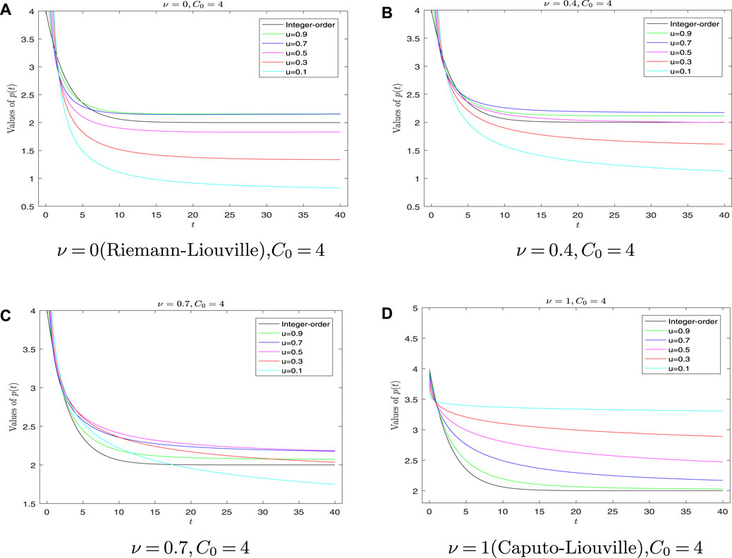
FIGURE 2. Graph of p(t) for different values of fractional-order μ with C₀> p_e. (A) Graph of p(t) with v = 0 (Riemann-Liouville), C₀ = 4. (B) Graph of p(t) with v = 0.4, C₀ = 4. (C) Graph of p(t) with v = 0.7, C₀ = 4. (D) Graph of p(t) with v = 1 (Caputo-Liouville), C₀ = 4.

FIGURE 3

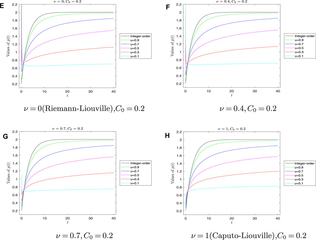
FIGURE 3. Graph of p(t) for different values of fractional-order μ with C₀< p_e. (E) Graph of p(t) with v = 0 (Riemann-Liouville), C₀ = 0.2. (F) Graph of p(t) with v = 0.4, C₀ = 0.2. (G) Graph of p(t) with v = 0.7, C₀ = 0.2. (H) Graph of p(t) with v = 1 (Caputo-Liouville), C₀ = 0.2.

After some calculation, it can be verified that when C₀ > p_e, p(t) has the memoryless property or Markov property. First, the graphs in Figure 2 concerning the R–L fractional derivative (ν = 0) and the families of Hilfer fractional derivative with types ν for which 0 < ν < 1 are divergent and unstable at the beginning t₀ by observing Figure 2 and Figure 3. Under the condition of C₀ > p_e, the curve of p(t) goes down very fast at the initial time t₀ and then p(t) becomes stable along with the increase in t; finally, p(t) converges to the equilibrium point p_e decreasingly. On the other hand, the value of p(t) drops rapidly in the case of C₀ < p_e in a very short period of time near t₀. However, the curve of p(t) increases again and becomes stable with the increase in t. In the end, it converges to the equilibrium p_e increasingly. Second, the smaller the μ of the fractional order is, the slower the p(t) converges to p_e. Third, the image of the C–L fractional derivative (ν = 1) is different from that of the R–L fractional derivative (ν = 0) and the families of Hilfer fractional derivative with types 0 < ν < 1, which seems to be more consistent with the derivative of integral order.

Case 2: This case discusses different types of fractional derivatives of p(t). We let the fractional-order μ be fixed first, such as setting μ = 0.1, 0.4, 0.7, 1 and C₀ = 4, 0.2 remain unchanged as previously mentioned. The case of C₀ = 4 > p_e is shown in Figure 4. The case of C₀ = 0.2 < p_e is shown in Figure 5.

FIGURE 4

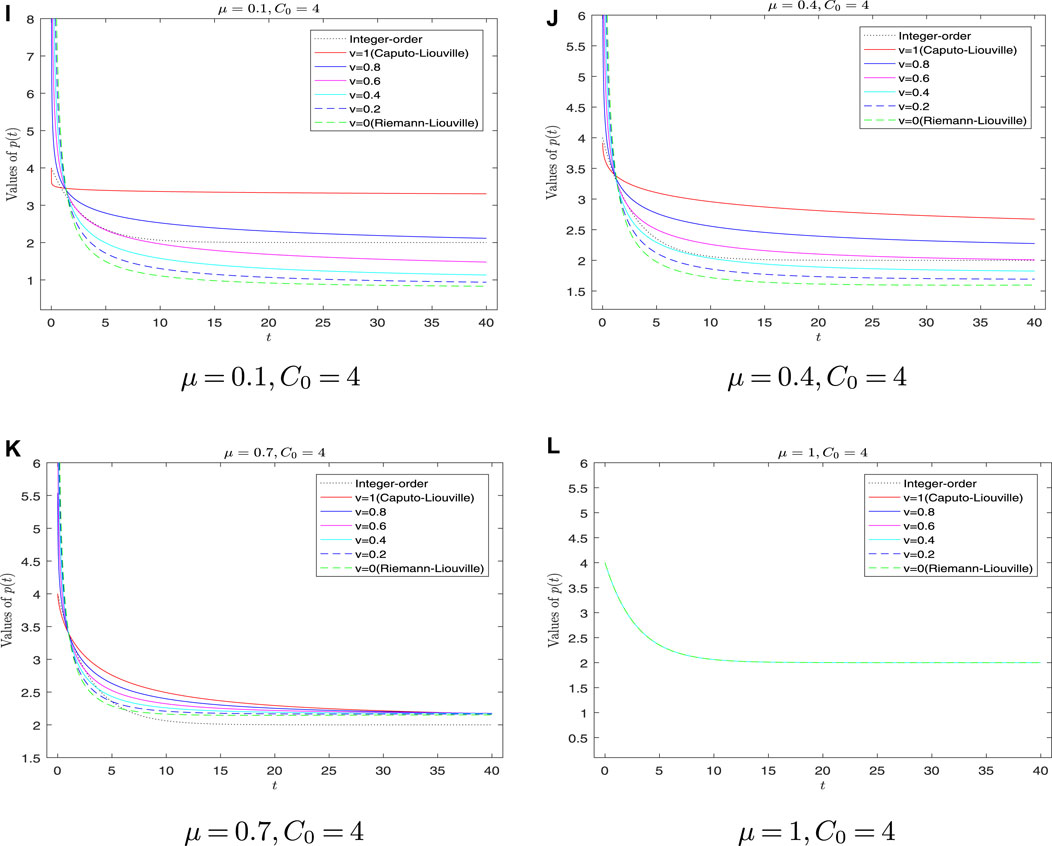
FIGURE 4. Graph of p(t) for different types of fractional derivatives with C₀> p_e. (I) Graph of p(t) with μ = 0.1, C₀ = 4. (J) Graph of p(t) with μ = 0.4, C₀ = 4. (K) Graph of p(t) with μ = 0.7, C₀ = 4. (L) Graph of p(t) with μ = 1, C₀ = 4.

FIGURE 5

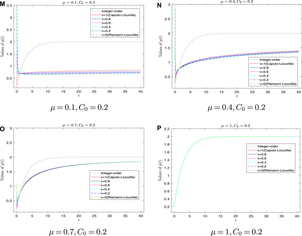
FIGURE 5. Graph of p(t) for different types of fractional derivatives with C₀< p_e. (M) Graph of p(t) with μ = 0.1, C₀ = 0.2. (N) Graph of p(t) with μ = 0.4, C₀ = 0.2. (O) Graph of p(t) with μ = 0.7, C₀ = 0.2. (P) Graph of p(t) with μ = 1, C₀ = 0.2.

Before the discussion, we give two forms of $\left(D_{a\pm }^{\mu ,\nu }p\right)(x)$ when μ = 0 and μ = 1. According to (7) and (8), we have

$\left(D_{a\pm }^{\mu ,\nu }p\right)\left(x\right)=\left\{\begin{array}{cc}\hfill & \left(\pm {}^{RL}I_{a\pm }^{\nu }\frac{d}{dx}\left({}^{RL}I_{a\pm }^{\left(1-\nu \right)}p\right)\right)\left(x\right)=p\left(x\right),\mu =0,\hfill \\ \hfill & \left(\pm {}^{RL}I_{a\pm }^0\frac{d}{dx}\left({}^{RL}I_{a\pm }^{0}p\right)\right)\left(x\right)=p^{\prime }\left(x\right),\mu =1.\hfill \end{array}\right.$

If μ = 0, model (18) turns into

$\left\{\begin{array}{cc}\hfill D\left(t\right)& =a+cp\left(t\right),\hfill \\ \hfill S\left(t\right)& =a_1+c_{1}p\left(t\right),\hfill \\ \hfill D\left(t\right)& =S\left(t\right).\hfill \end{array}\right.(25)$

It can be found that $p(t)=\frac{a_1-a}{c-c_1}$ is the solution of (25) with c ≠ c₁.

From Figure 4 and Figure 5, we can find that, as μ decreases (μ → 0), the curves of p(t) with C–L fractional derivative become more vertical, which is consistent with model (25). Second, if μ = 1, the fractional derivative turns into the ordinary derivative, so the curves (integer-order and types ν for which ν = 0, 0.2, 0.4, 0.6, 0.8, 1) in Figure 4 and Figure 5D coincide with each other, which ensures the compatibility of our model. Third, Figures 4B, C, and Figures 5B, C show that the higher the fractional derivative order μ, the faster the p(t) converges to p_e. Finally, we can also verify Case 1 from Figure 5A of Case 2.

6 Conclusion

This study focuses on exploring the solution of the cobweb economic model by integrating the Hilfer fractional derivative $D_{a+}^{\mu ,\nu }$ into both the demand and supply functions and the Markov process. By manipulating the parameters present in the model, a range of cobweb models can be created, each associated with different types of fractional derivatives and fractional orders. To obtain analytical solutions for these cobweb models, we use the Laplace transform method. Additionally, we conduct a thorough stability analysis of these solutions and compute the equilibrium points. For this purpose, we can gain a better understanding of the dynamics of the cobweb economic model under different conditions and parameters, which can be useful for policymakers and economists in making informed decisions.

The results of our investigation demonstrate that the C–L fractional derivative, when compared to the R–L fractional derivative and the families of Hilfer fractional derivatives with types 0 < ν < 1, displays a high level of practical robustness and retains a significant number of desirable properties that are characteristic of integer derivatives. As a result, the C–L fractional derivative emerges as a more appropriate choice for effectively modeling and analyzing the cobweb economic model. Our findings suggest that the C–L fractional derivative can provide more accurate and reliable results, making it a valuable tool for economists and policymakers in understanding the dynamics of economic systems. The outcomes contribute to the ongoing development of fractional calculus and its applications in economic modeling, providing insights into the behavior of complex economic systems.

Overall, this study has made substantial contributions to the field by examining the behavior of the cobweb economic model when influenced by the Hilfer fractional derivative in both the demand and supply functions. The analytical solutions obtained, along with the stability analysis and computation of equilibrium points, have yielded valuable insights into the dynamic nature of the model. Moreover, our findings highlight the numerous advantages offered by the C–L fractional derivative, further emphasizing its practical significance and its ability to preserve key properties commonly associated with traditional, integer derivatives. These findings have important implications for economic modeling and analysis, as they provide economists and policymakers with a more accurate and reliable tool for understanding and predicting the behavior of economic systems. By shedding light on the benefits of the C–L fractional derivative, this study contributes to the advancement of fractional calculus and its applications in the field of economics.

Data availability statement

The original contributions presented in the study are included in the article/Supplementary Material; further inquiries can be directed to the corresponding author.

Author contributions

XQ: conceptualization, data curation, methodology, resources, and writing–original draft. ZR: conceptualization, data curation, formal analysis, funding acquisition, visualization, and writing–review and editing. WP: conceptualization, data curation, methodology, supervision, and writing–review and editing.

Funding

The authors declare financial support was received for the research, authorship, and/or publication of this article. This research was funded by the university Key Project of Natural Science Foundation of Anhui Province grants 2023AH052106, KJ2021A1032, KJ2019A0683, and KJ2021A1031, Key Project of Natural Science Foundation of Chaohu University grant XLZ-202201, Key Construction Discipline of Chaohu University grants kj22zdjsxk01,kj22yjzx05, and kj22xjzz01.

Conflict of interest

The authors declare that the research was conducted in the absence of any commercial or financial relationships that could be construed as a potential conflict of interest.

Publisher’s note

All claims expressed in this article are solely those of the authors and do not necessarily represent those of their affiliated organizations, or those of the publisher, the editors, and the reviewers. Any product that may be evaluated in this article, or claim that may be made by its manufacturer, is not guaranteed or endorsed by the publisher.

Supplementary material

The Supplementary Material for this article can be found online at: https://www.frontiersin.org/articles/10.3389/fphy.2023.1266860/full#supplementary-material

References

1. Hilfer R. Applications of fractional calculus in physics. Singapore: World Scientific (2000).

Google Scholar

2. Samko SG, Kilbas AA, Oleg IM. Fractional integrals and derivatives: theory and applications. Switzerland: Gordon and breach science publishers, Yverdon Yverdon-les-Bains (1993).

Google Scholar

3. Kilbas AA, Srivastava HM, Trujillo JJ. Theory and applications of fractional differential equations. Amsterdam, Netherlands: Elsevier (2006).

Google Scholar

4. Almeida R, da Cruz AB, Martins N, Monteiro MTT. An epidemiological mseir model described by the caputo fractional derivative. Int J Dyn Control (2019) 7(2):776–84. doi:10.1007/s40435-018-0492-1

CrossRef Full Text | Google Scholar

5. Hashemi MS, Dumitru B, Parto-Haghighi M, Darvishi E. Solving the time-fractional diffusion equation using a lie group integrator (2015). doi:10.2298/TSCI15S1S77H

CrossRef Full Text | Google Scholar

6. Hristov J. Transient heat diffusion with a non-singular fading memory: From the cattaneo constitutive equation with jeffrey kernel to the caputo-fabrizio time-fractional derivative. Therm Sci (2016) 20(2):757–62. doi:10.2298/TSCI160112019H

CrossRef Full Text | Google Scholar

7. Hristov J. Fourth-order fractional diffusion model of thermal grooving: Integral approach to approximate closed form solution of the mullins model. Math Model Nat Phenomena (2018) 13(1):6. doi:10.1051/mmnp/2017080

CrossRef Full Text | Google Scholar

8. Traore A, Sene N. Model of economic growth in the context of fractional derivative. Alexandria Eng J (2020) 59(6):4843–50. doi:10.1016/j.aej.2020.08.047

CrossRef Full Text | Google Scholar

9. Sene N. Integral balance methods for Stokes’ first equation described by the left generalized fractional derivative. Physics (2019) 1(1):154–66. doi:10.3390/physics1010015

CrossRef Full Text | Google Scholar

10. Sene N. Second-grade fluid model with caputo–liouville generalized fractional derivative. Chaos, Solitons and Fractals (2020) 133:109631. doi:10.1016/j.chaos.2020.109631

CrossRef Full Text | Google Scholar

11. Sene N. Stokes’ first problem for heated flat plate with atangana–baleanu fractional derivative. Chaos, Solitons and Fractals (2018) 117:68–75. doi:10.1016/j.chaos.2018.10.014

CrossRef Full Text | Google Scholar

12. Avci D, Ozdemir N, Yavuz M. Fractional optimal control of diffusive transport acting on a spherical region. In: Methods of mathematical modelling. Boca Raton, Florida, CRC Press (2019). p. 63–82.

CrossRef Full Text | Google Scholar

13. Asjad MI, Ullah N, Rehman HU, Gia TN. Novel soliton solutions to the atangana-baleanu fractional system of equations for the isalws. Open Phys (2021) 19(1):770–9. doi:10.1515/phys-2021-0085

CrossRef Full Text | Google Scholar

14. Jan R, Shah Z, Deebani W, Alzahrani E. Analysis and dynamical behavior of a novel dengue model via fractional calculus. Int J Biomathematics (2022) 15(06):2250036. doi:10.1142/S179352452250036X

CrossRef Full Text | Google Scholar

15. Hilfer R, Luchko Y, Tomovski Z. Operational method for the solution of fractional differential equations with generalized riemann-liouville fractional derivatives. Fract Calc Appl Anal (2009) 12(3):299–318.

Google Scholar

16. Sene N. Exponential form for lyapunov function and stability analysis of the fractional differential equations. J Math Comput Sci (2018) 18(4):388–97. doi:10.22436/jmcs.018.04.01

CrossRef Full Text | Google Scholar

17. Priyadharsini S. Stability of fractional neutral and integrodifferential systems. J Fract Calc Appl (2016) 7(1):87–102. doi:10.21608/jfca.2016.308374

CrossRef Full Text | Google Scholar

18. Owolabi KM, Hammouch Z. Mathematical modeling and analysis of two-variable system with noninteger-order derivative. Chaos: Interdiscip J Nonlinear Sci (2019) 29(1):013145. doi:10.1063/1.5086909

PubMed Abstract | CrossRef Full Text | Google Scholar

19. Sene N. Analytical solutions of hristov diffusion equations with non-singular fractional derivatives. Chaos: Interdiscip J Nonlinear Sci (2019) 29(2):023112. doi:10.1063/1.5082645

PubMed Abstract | CrossRef Full Text | Google Scholar

20. Abdeljawad T, Mert R, Peterson A. Sturm liouville equations in the frame of fractional operators with exponential kernels and their discrete versions. Quaestiones Mathematicae (2019) 42(9):1271–89. doi:10.2989/16073606.2018.1514540

CrossRef Full Text | Google Scholar

21. Bohner M, Hatipoğlu VF. Cobweb model with conformable fractional derivatives. Math Methods Appl Sci (2018) 41(18):9010–7. doi:10.1002/mma.4846

CrossRef Full Text | Google Scholar

22. Bohner M, Hatipoğlu VF. Dynamic cobweb models with conformable fractional derivatives. Nonlinear Anal Hybrid Syst (2019) 32:157–67. doi:10.1016/j.nahs.2018.09.004

CrossRef Full Text | Google Scholar

23. Bagley RL. On the fractional order initial value problem and its engineering applications. In: International conference proceedings. Tokyo: Mdpi (1990). p. 12–20.

Google Scholar

24. Beyer H, Kempfle S. Definition of physically consistent damping laws with fractional derivatives. ZAMM-Journal Appl Maths Mechanics/Zeitschrift für Angew Mathematik Mechanik (1995) 75(8):623–35. doi:10.1002/zamm.19950750820

CrossRef Full Text | Google Scholar

25. Miller KS, Ross B. An introduction to the fractional calculus and fractional differential equations. Hoboken, New Jersey: Wiley (1993).

Google Scholar

26. Younis M, Hamood UR, Syed Tahir RR, Syed Amer M. Dark and singular optical solitons perturbation with fractional temporal evolution. Superlattices and Microstructures (2017) 104:525–31. doi:10.1016/j.spmi.2017.03.006

CrossRef Full Text | Google Scholar

27. Jan A, Jan R, Khan H, Zobaer MS, Shah R. Fractional-order dynamics of rift valley fever in ruminant host with vaccination. Commun Math Biol Neurosci (2020).

Google Scholar

28. Ur Rehman H, Imran MA, Ullah N, Ali A. On solutions of the newell-whitehead-segel equation and zeldovich equation. Math Methods Appl Sci (2021) 44(8):7134–49. doi:10.1002/mma.7249

CrossRef Full Text | Google Scholar

29. Rehman HU, Mustafa I, Muhammad IA, Azka H, Qamar M. New soliton solutions for the space-time fractional modified third order korteweg–de vries equation. J Ocean Eng Sci (2022). doi:10.1016/j.joes.2022.05.032

CrossRef Full Text | Google Scholar

30. Acay B, Bas E, Abdeljawad T. Fractional economic models based on market equilibrium in the frame of different type kernels. Chaos, Solitons and Fractals (2020) 130:109438. doi:10.1016/j.chaos.2019.109438

CrossRef Full Text | Google Scholar

31. Lin Z, Wang H. Modeling and application of fractional-order economic growth model with time delay. Fractal and Fractional (2021) 5(3):74. doi:10.3390/fractalfract5030074

CrossRef Full Text | Google Scholar

32. Shah Z, Bonyah E, Alzahrani E, Jan R, Alreshidi NA. Chaotic phenomena and oscillations in dynamical behaviour of financial system via fractional calculus. Complexity (2022) 2022. doi:10.1155/2022/8113760

CrossRef Full Text | Google Scholar

33. Luchko Y. Operational method in fractional calculus. Fract Calc Appl Anal (1999) 2(4):463–88.

Google Scholar

34. Tang T-Q, Shah Z, Jan R, Alzahrani E. Modeling the dynamics of tumor-immune cells interactions via fractional calculus. The Eur Phys J Plus (2022) 137(3):367. doi:10.1140/epjp/s13360-022-02591-0

CrossRef Full Text | Google Scholar

35. Yousefpour A, Jahanshahi H, Castillo O. Application of variable-order fractional calculus in neural networks: Where do we stand? Eur Phys J Spec Top (2022) 231(10):1753–6. doi:10.1140/epjs/s11734-022-00625-3

CrossRef Full Text | Google Scholar

36. Fulford G, Forrester P, Forrester PJ, Jones A. Modelling with differential and difference equations. Cambridge: Cambridge University Press (1997).

Google Scholar

37. Gandolfo G. Economic dynamics: Methods and models. Elsevier (1971).

Google Scholar

38. Kaldor N. A classificatory note on the determinateness of equilibrium. Rev Econ Stud (1934) 1(2):122–36. doi:10.2307/2967618

CrossRef Full Text | Google Scholar

39. Ezekiel M. The cobweb theorem. Q J Econ (1938) 52(2):255–80. doi:10.2307/1881734

CrossRef Full Text | Google Scholar

40. Srivastava HM, Raghavan D, Nagarajan S. A comparative study of the stability of some fractional-order cobweb economic models. Revista de La Real Academia de Ciencias Exactas, Físicas y Naturales Serie A Matemáticas (2022) 116(3):1–20. doi:10.1007/s13398-022-01239-z

CrossRef Full Text | Google Scholar

41. Chen C, Bohner M, Jia B. Caputo fractional continuous cobweb models. J Comput Appl Maths (2020) 374:112734. doi:10.1016/j.cam.2020.112734

CrossRef Full Text | Google Scholar

42. Sar EY, Giresunlu IB. Fractional differential equations. Pramana–j Phys (2016) 87:17.

Google Scholar

43. Jarad F, Abdeljawad T. A modified laplace transform for certain generalized fractional operators. Results Nonlinear Anal (2018) 1(2):88–98.

Google Scholar

44. Tomovski Ž, Hilfer R, Srivastava HM. Fractional and operational calculus with generalized fractional derivative operators and mittag–leffler type functions. Integral Transforms Spec Functions (2010) 21(11):797–814. doi:10.1080/10652461003675737

CrossRef Full Text | Google Scholar

45. Hilfer R. Experimental evidence for fractional time evolution in glass forming materials. Chem Phys (2002) 284(1-2):399–408. doi:10.1016/S0301-0104(02)00670-5

CrossRef Full Text | Google Scholar

46. Wright EM. The asymptotic expansion of integral functions defined by taylor series. Philos Trans R Soc Lond Ser A, Math Phys Sci (1940) 238(795):423–51.

Google Scholar

47. Gorenflo R, Kilbas AA, Mainardi F, Sergei VR. Mittag-Leffler functions, related topics and applications. Berlin, Germany: Springer (2020).

Google Scholar

48. Lavault C. Integral representations and asymptotic behaviour of a mittag-leffler type function of two variables. Adv Operator Theor (2018) 3(2):365–73. doi:10.15352/APT.1705-1167

CrossRef Full Text | Google Scholar

49. Bohner M, Jonnalagadda JM. Discrete fractional cobweb models. Chaos, Solitons and Fractals (2022) 162:112451. doi:10.1016/j.chaos.2022.112451

CrossRef Full Text | Google Scholar