High-energy X-ray spectrum reconstruction: solving the inverse problem from optimized multi-material transmission measurements

Reconstructing the unknown spectrum of a given X-ray source is a common problem in a wide range of X-ray imaging tasks. For high-energy sources, transmission measurements are mostly used to recover the X-ray spectrum, as a solution to an inverse problem. While this inverse problem is usually under-determined, ill-posedness can be reduced by improving the choice of transmission measurements. A recently proposed approach optimizes custom thicknesses of calibration materials used to generate transmission measurements, employing a genetic algorithm to minimize the condition number of the system matrix before inversion. In this paper, we generalize the proposed approach to multiple calibration materials and show a much larger decrease of the condition number of the system matrix than thickness-only optimization. Additionally, the spectrum reconstruction pipeline is tested in a simulation study with a challenging high-energy Bremsstrahlung X-ray source encountered in Linear Induction Accelerators with strong scatter noise. Using this approach, a realistic noise level is obtained on measurements. A generic anti-scatter grid is designed to reduce noise to an acceptable -yet still high-noise range. A novel noise-robust reconstruction method is then presented, which shows much less sensitive to initialization than common expectation-maximization approaches, enables a precise choice of spectrum resolution and a controlled injection of prior knowledge of the X-ray spectrum.

1 Introduction

The reconstruction of the unknown spectrum of a given X-ray source is a common problem in a wide range of X-ray imaging tasks [1, 2]. If the source flux is low, spectrometers are usually preferred to estimate the spectrum. If a very precise modeling of the source is available, a good knowledge of the X-ray spectrum can be obtained, provided that the model input parameters, such as voltage, are measured precisely enough during the pulse [3]. When none of the two previous conditions are met, transmission measurements are most frequently used to recover the X-ray spectrum, as a solution to an inverse problem [4–7].

This inverse problem is usually under-determined, because a high resolution of the reconstructed spectrum is required. It is also ill-conditioned, making the spectral estimation unstable and very sensitive to noise. The ill-posedness of this inverse problem can be reduced using a parametric model of the reconstructed spectrum [8, 9]. However, these model-based methods restrict, by design, the space of possible solutions, thus requiring a fine and general enough physical modelling of the spectrum prior to reconstruction.

Another way to reduce ill-posedness is to improve the quality of the set of transmission measurements. In particular, the recent approach described in [10] proposed to compute custom thicknesses of calibration materials used to generate transmission measurements, by optimizing on the condition number of the system matrix used for inversion. Using a genetic algorithm, the interest of optimized measurements to reconstruct spectra was demonstrated, in comparison with common linear slab phantoms.

While the approach proved to be very efficient for the configurations tested in [10], their simulation study was restricted to unrealistically small amounts of Poisson noise, and relatively low-energy spectra. In this work, a challenging high-energy Schiff spectrum [11] is used to simulate transmission measurements using the Monte-Carlo N-Particle code (MCNP4C) with realistic noise levels. The Schiff spectrum is a typical model for thin-target Bremsstrahlung spectra encountered in radiographic sources based on Linear Induction Accelerators (LIA), used to perform high-energy flash X-ray imaging [12]. We show that the method presented in [10] is not readily applicable to this real-world reconstruction problem. Three improvements are thus proposed to obtain a robust spectrum reconstruction. Firstly, the transmission measurement optimization, reduced to variations of material thicknesses in [10], is extended to multiple materials by modifying the genetic algorithm. We show that using multiple materials yields a much larger decrease of the condition number of the system matrix than thickness-only optimization. Secondly, instead of a generic Poisson noise, a realistic simulated scatter noise is used to evaluate the ability to recover the spectrum. Using this approach, we observe a much higher noise level on measurements, which makes the design of a noise reduction setup mandatory. As such, an anti-scatter grid is proposed, reducing noise to an acceptable range for spectrum reconstruction, but still much higher than noise levels encountered in [10]. Thirdly, once measurements are optimized and the experimental setup is fixed, a novel reconstruction method is presented, which shows much less sensitive to initialization than expectation-maximization approaches [10], enables a precise choice of spectrum resolution and a controlled injection of prior knowledge of the X-ray spectrum.

2 Methods

2.1 Transmission measurement model

As illustrated in Figure 1, two types of transmission measurements are considered, which correspond to the two experimental configurations tested in this study. In a given experiment, the setup is made of M slabs illuminated by the X-ray source. Behind each slab, a detector is placed to measure the fluence (the detector response function is ideal), which gives us M measurements from which we can infer the X-ray source spectrum. Each slab can be made of K layers of different materials (left side of Figure 1) or just one material (right side of Figure 1).

FIGURE 1

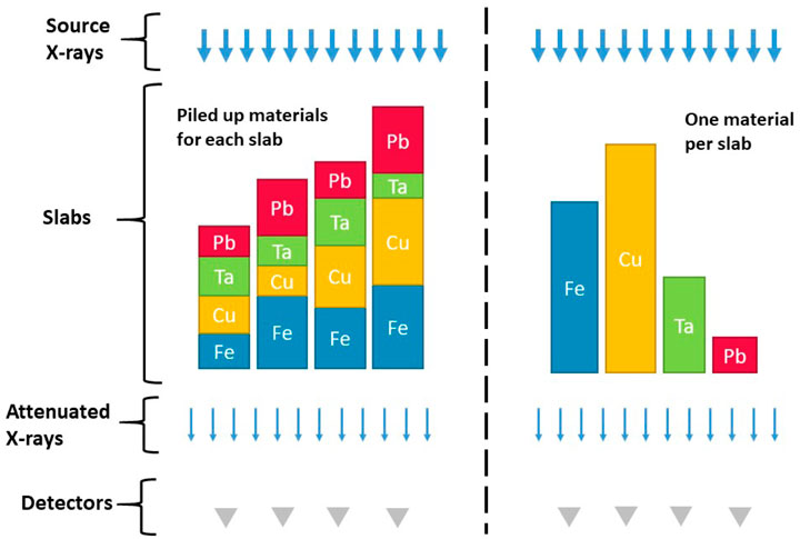
FIGURE 1. Illustration of the two configurations considered for 4 measurement slabs. A detector is placed behind each slab to measure the attenuated signal.

In what follows, the detector spectral response D(E) is not accounted for and taken as unity. For each measurement, the forward transmission model is given by the Beer-Lambert law. Given an X-ray source with spectrum S(E), the transmitted intensity I of a measurement writes

$I={\int }_{E}S\left(E\right)D\left(E\right)e^{-l\mu \left(E\right)}dE(1)$

where l is the thickness and μ(E) the linear attenuation coefficient (taken from the NIST database [13]) of the material used for this measurement.

2.1.1 One material per measurement

This configuration corresponds to the right side of Figure 1. For M measurements y_i and with an even discretization of the spectrum into N bins, the forward problem can be cast into a set of linear equations

$y_i=\sum _{j=1}^N{e}^{-l_i{\mu }_{i,j}}{s}_j,i\in \left[\left[1,M\right]\right],j\in \left[\left[1,N\right]\right](2)$

where l_i is the thickness of the ith measurement and μ_i,j is the linear attenuation coefficient value for the ith measurement at the discrete energy level j.

Eq. 2 is conveniently put in the matrix form as

$\mathbf{y}=A\times \mathbf{s}(3)$

with $\mathbf{y}=(y_i)\in {\mathbb{R}}^M$ the vector of transmission measurements, $\mathbf{s}=(s_j)\in {\mathbb{R}}^N$ the vector of the discretized spectrum and $A=(e^{-l_i{\mu }_{i,j}})\in {\mathbb{R}}^{M\times N}$ the forward system matrix.

2.1.2 Multiple materials per measurement

This configuration is illustrated at the left side of Figure 1. Each measurement contains K layers of distinct materials. Without any loss of generality, we consider that each measurement contains the same number of layers with the same material order. Only the thickness of each material layer is changed, and can be set to zero. With this assumption, the attenuation coefficient no longer depends on the measurement number i. The transmitted intensity y_i for the ith measurement thus writes

$y_i=\sum _{j=1}^N\prod _{k=1}^K{e}^{-l_{i,k}{\mu }_{k,j}}{s}_j,i\in \left[\left[1,M\right]\right],j\in \left[\left[1,N\right]\right],k\in \left[\left[1,K\right]\right](4)$

where l_i,k is the thickness of the kth layer of the ith measurement and μ_k,j(E) is the linear attenuation coefficient of the material k at energy level j. The forward system matrix in Eq. 3 is modified as $A=(e^{-{\sum }_k{l}_{i,k}{\mu }_{k,j}})\in {\mathbb{R}}^{M\times N}$.

2.2 Multi-material thickness optimization

First, let us summarize the methodology and main results in [10]. The authors worked with one material per slab, as illustrated by the right side of Figure 1, and used a genetic algorithm to optimize the matrix condition number with respect to the thickness and material of each slab. They found that the matrix condition number tend to increase with the number of measurements and that the optimal thickness arrangement follows an exponential sequence. In particular, these findings show that what is usually done (i.e., thickness follows a linear sequence and a great number of measurements is used) tend to increase the matrix condition number by orders of magnitude. An expectation-maximization (EM) algorithm is then used to invert the system and find the spectrum. Moreover, this method was tested to be robust against relatively low levels of Poisson noise. However, much higher noise levels are routinely encountered in experiments. At such noise levels, we believe that a new method is needed.

Using multiple materials in transmission measurements implies some modifications to the thickness optimization genetic algorithm described in [10]. Two optimizations with slightly different implementations, corresponding to the two types of transmission measurements discussed above, are here considered and tested.

2.2.1 Multiple materials per measurement

When multiple piled up materials are allowed for each measurement, the genetic algorithm optimizes on two-dimensional matrices of size M × K instead of one-dimensional vectors in the single material case. Each cell of the matrices contains the current thickness of the column’s corresponding material for the line’s corresponding measurement. In comparison with [10], the main steps of the genetic optimization are modified as follows.

• Initialization: N_pop matrices are initialized with a randomly chosen value in each cell, such that the sum on each row (i.e., the total thickness of the corresponding measurement slab) remains in a chosen interval [l_min, l_max]

• Crossover: the crossover formula used in [10] is applied similarly to the rows of the system matrix

• Mutation: instead of simply modifying the value of the mutated cell as in [10], the sum of values on the row, corresponding to the total thickness, is modified as well as the proportion of materials

2.2.2 One material per measurement

When only one material is allowed per measurement, two-dimensional M × K matrices are also used but with only one non-zero value per row, at the column corresponding to the employed material. The main steps of the genetic optimization are modified as follows.

• Initialization: N_pop matrices are initialized with a randomly chosen value in only 1 cell per row, and the other cells are initialized to zero

• Crossover: If the two parents are using the same material, the situation refers to the case of [10]. Otherwise, the two children receive one material each, with thickness values crossed with the same formula

• Mutation: Each mutation on a row also has a probability of changing the material used for the corresponding measurement

2.3 Geometry design and simulation

A basic MCNP4C geometry was built for each set of measurements. Transmission measurement phantoms were represented as cylinders of known thicknesses and radii. Cylinders axes are aiming at the photon source, which is modeled as a point source located 180 cm away from the phantoms. A Schiff spectrum, corresponding to a maximum electron energy of 20 MeV, incident on a 1.2 mm thick tantalum target, is used. The photons are emitted within a cone with a constant angular distribution, chosen in order to cover all the measurement devices. Both photon and electron interactions are modeled, so as to accurately account for scattering. The filling medium is air. All these parameters were chosen to be as close as possible to reality.

The detectors in the simulation are modeled as simple fluence tallies, placed behind each measurement slab. Consistent modeling of detectors in the simulation and accounting for their spectral responses in the optimization process, is left to future work.

As mentioned earlier, the MCNP4C simulation accounts for the presence of scatter noise in the measurements, produced during the passage of X-rays through materials. A specific simulation setup was designed to reduce this scatter noise and obtain clean enough measurements for the spectrum reconstruction.

The proximity between measurement slabs leads to an increase in scatter noise due to cross-talk effects. As such, the first approach employed to decrease scatter noise was to optimize the placement of the measurement slabs within the experimental setup and space them out in order to reduce the interaction between particles coming through the materials. The differential evolution algorithm [14] was used to compute the optimal placement of M points constrained in a circle by minimizing the electrostatic potential between them.

To further reduce this noise, a specific anti-scatter grid was designed. This grid consists of a 20 cm deep lead layer between the measurement slabs and the dose sensors. Cylinders of small radius are carved in the lead behind each measurement slab in order to absorb all particles except source photons, yielding the expected signal.

2.4 Reconstruction algorithm

2.4.1 Adaptive resampling based on a typical spectrum

Prior to the reconstruction algorithm itself, a preliminary step of dimension reduction is realized on a typical spectrum presenting roughly the same characteristics as the unknown spectrum. As shown in Figure 2, by sampling uniformly from the cumulative integral of this typical spectrum’s derivative, an approximately optimal choice of the N energy bins is obtained, allowing an efficient spectrum representation, later employed during the optimization process of the reconstruction.

FIGURE 2

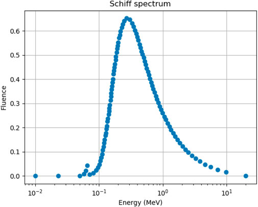
FIGURE 2. Typical Schiff spectrum optimally discretized to N =100 energy points. The spectrum is normalized to unity.

2.4.2 Spectrum reconstruction as an interpolation

The spectrum is reconstructed on the optimal energy sampling presented above, using experimental or simulated measurements y. A candidate spectrum s_cand is initialized and then modified during the optimization process. The measurements computed through the forward model y_cand = A ×s_cand are expected to be as close to y as possible.

The optimization problem for the spectrum reconstruction thus writes:

$\underset{{\mathbf{s}}_{\mathit{cand}}}{\mathrm{argmin}}\Vert \mathbf{y}-A\times {\mathbf{s}}_{\mathit{cand}}{\Vert }^2(5)$

A straightforward method would consist in performing a spectrum discretization over the optimal energy sampling values E₁, …, E_N where N is usually large to obtain a good resolution of the spectrum. However, a large N increases the degrees of freedom and makes the optimization process harder. It is therefore necessary to reduce the number of parameters used to describe the spectrum. The method chosen here is to sample the spectrum with a small number P of interpolation points. This requires the spectrum to be continuous and deprived of high variation peaks, which is a general feature of high-energy Bremsstrahlung spectra.

As shown in Figure 3, the spectrum is thus fully described by P interpolation points, which coordinates can evolve both in energy and magnitude (e.g., 2P degrees of freedom). At each optimization step, the points are interpolated by a piecewise cubic polynomial function [15], then projected over the N energy intervals. y_cand is then computed and new values of coordinates for the interpolation points can be determined.

FIGURE 3

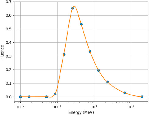
FIGURE 3. Schiff spectrum interpolated by P = 12 interpolation points distributed in the energy interval.

2.4.3 Reconstruction algorithm

A trust-region algorithm for constrained optimization [16] is used to compute the interpolation points corresponding to the approximated spectrum. Minimum and maximum energy levels are enforced, based on a known low energy cut-off and the maximum energy of electrons. The spectrum magnitude is constrained using a simple step function. In addition to this restriction, the spectrum is normalized by its integral during each step of the optimization process.

For this algorithm, the P abscissa of the interpolation points are fixed, which improves optimization performances and decreases execution time. However, other algorithms might be more efficient with the abscissa taken as additional degrees of freedom. In the case of this study, these abscissa values are taken as evenly spaced inside the energy interval, in logarithmic scale. The optimization algorithm is then applied to the P magnitudes of the interpolation points, with a fixed number of iterations.

3 Results

3.1 Impact of multiple materials

A comparison between our multi-material genetic algorithm and the version implemented in [10] was performed using the same setup. A number of M = 8 measurements was fixed, N = 100 energy bins and K = 4 materials (iron, copper, tantalum and lead) were used. For a fair comparison, all other hyper-parameters, including the number of generations, the population size, the crossover and mutation probabilities, the target distribution mean and the best fitness boosting factor, were kept identical to [10].

3.1.1 Algorithms performance

The work done in [10] led to a great reduction in orders of magnitude of the forward matrix condition number, and highlighted an exponential distribution of thicknesses for the optimal measurement set using one material. Using this one-material genetic algorithm, the optimal arrangement of thicknesses plotted on Figure 4A was obtained, with a condition number of 1.8 × 10⁶.

FIGURE 4

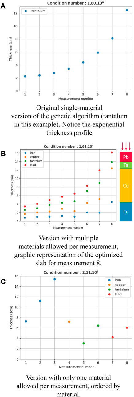
FIGURE 4. Optimal arrangement of thicknesses and achieved condition number for the different versions of the genetic algorithm.

Figure 4B displays the results obtained using the first type of transmission measurements with several materials, described in Section 2.2.1. When multiple piled up materials are allowed per measurement, a significant improvement of the previous results is observed, with a further reduced condition number of 1.61 × 10⁴.

Figure 4C shows the results obtained using a single material per measurement. With this second version of the algorithm presented in 2.2.2, an even greater improvement is observed with a highly reduced condition number of 2.11 × 10³.

3.1.2 Stability of the optimization

Regardless of the performance of the different algorithms, another main goal of the proposed algorithms is to ensure a good stability of the optimized measurements. To compare the stability of the multi-material algorithms developed in this study, both were executed several times with the same parameters. The set of materials obtained for each optimization was then plotted.

Results are shown in Figure 5. In Figure 5A where multiple materials per measurement are allowed, the mean thickness value and the standard deviation of each piled up material for each measurement are plotted. However, in Figure 5B where only one material is allowed per measurement, the plots have to be separated because a given measurement can correspond to different materials for different optimizations.

FIGURE 5

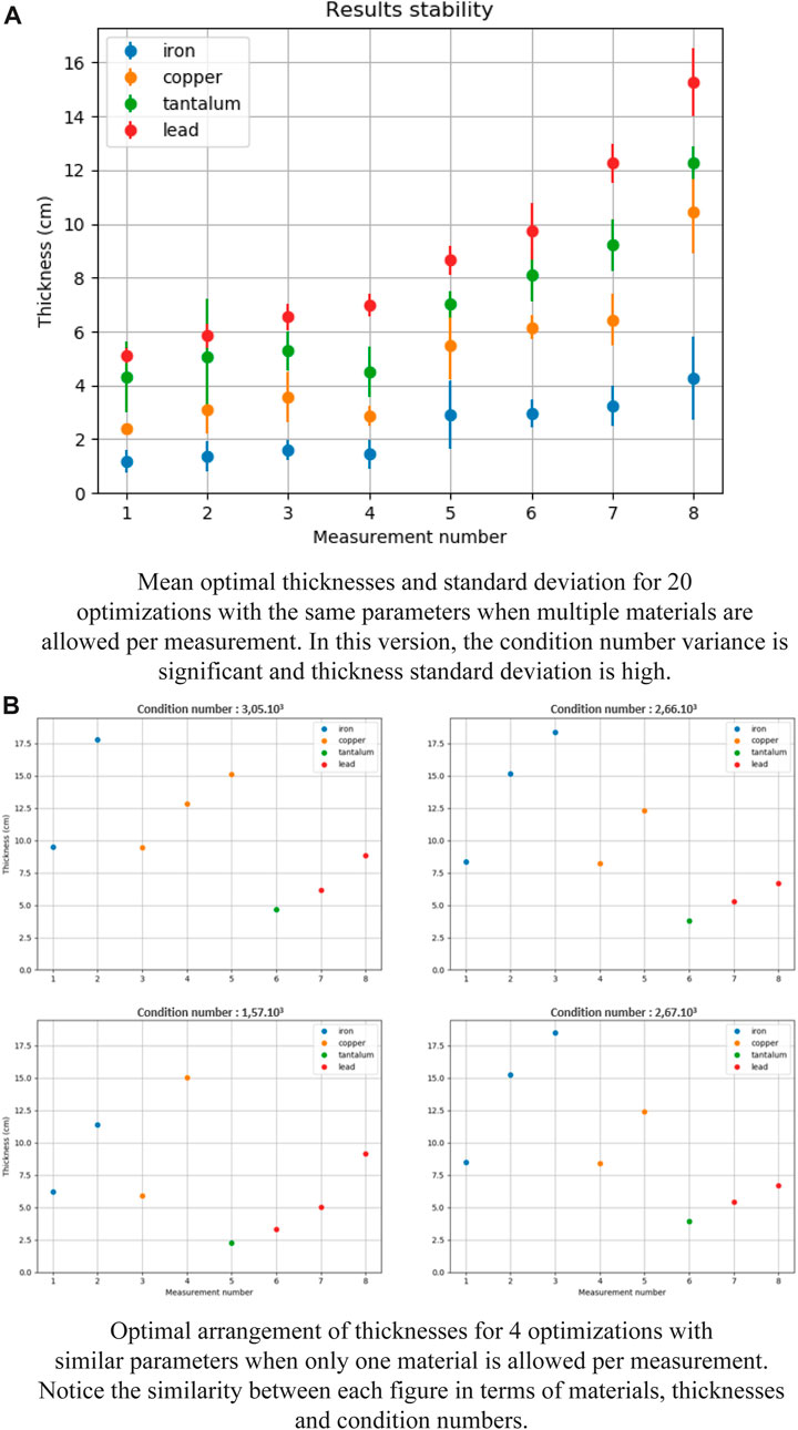
FIGURE 5. Stability study for both versions of the multi-material genetic algorithm. The version when only one material is allowed per measurement (B) is more stable and is hence preferred.

The result of the stability comparison is clear. As illustrated on Figure 5A, the algorithm version with piled up materials is quite unstable, with a significant standard deviation on material thicknesses between experiments and a strong variance on the condition number. Conversely, for the algorithm with only one material per measurement, the stability is satisfying. As shown in Figure 5B, each measurement is attributed almost always the same material with the same thickness across experiments. The reduction of the research space size thus plays a key role in the stability improvement.

3.2 Reduction of scatter noise

Different geometric configurations have been tested in MCNP4C to reduce scatter noise while keeping an easy-to-design setup. For each of them, a simulation was run using the measurement slabs returned by the one-material-per-measurement version of the genetic algorithm for M = 12 measurements. In this study we consider that scattered rays represent the entire measurement noise, which is a reasonable approximation. The Monte-Carlo simulation code allows the calculation of the theoretical unscattered rays along with the measurement of total (unscattered and scattered) rays. The objective is to design a configuration in which the measured total rays are as close to the theoretical direct rays as possible. Total and unscattered rays have been measured for each simulation and are plotted in Figure 6.

FIGURE 6

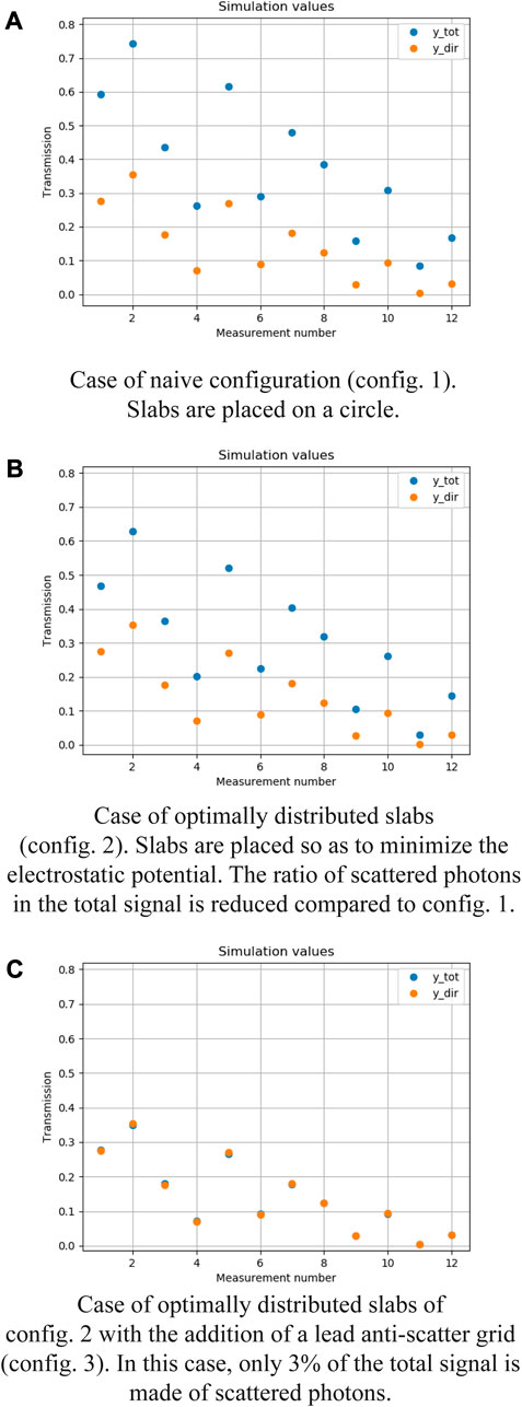
FIGURE 6. Total (y_tot) and direct (y_dir) measured rays for the 3 tested experimental configurations. Best results are obtained with configuration 3, using an anti-scatter grid.

Three configurations were tested: a straightforward design where measurement slabs were placed on the edge of a circle of given radius (config. 1, Figure 6A), a reworked configuration in which slabs were optimally distributed in a circle by minimizing the electrostatic potential between them (config. 2, Figure 6B), and a last design where a thick lead anti-scatter grid was added between the measurement slabs and the sensors of configuration 2 (config. 3, Figure 6C).

With configuration 2, the scatter noise was reduced by half compared to configuration 1. While significant, this reduction is not sufficient to exploit transmission measurements for spectrum reconstruction. Using an anti-scatter grid (configuration 3) reduces the scatter noise to an exploitable amount of around 3%, allowing the measurements to be used for the spectrum reconstruction.

3.3 Schiff spectrum reconstruction

3.3.1 Nominal configuration

In this study, the nominal configuration for the spectrum reconstruction consists in: M = 12 measurements, N = 100 energy intervals, K = 4 different materials (iron, copper, tantalum and lead), only one material allowed per measurement in the genetic measurement set optimization (hyperparameters: 500 generations, 1000 in population size), config. Three for the simulation configuration, and p = 10 interpolation points for the reconstruction algorithm.

For this nominal configuration, the reconstruction algorithm has been applied multiple times. Reconstructed spectrums (dotted lines) are plotted on Figure 7, along with the objective theoretical spectrum (solid black line).

FIGURE 7

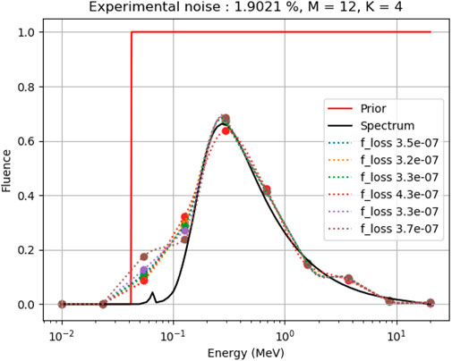
FIGURE 7. Spectrum reconstruction in the nominal configuration: prior function (red), source spectrum (black) and reconstructed spectrums (dotted lines). Values under 40 keV are not reconstructed and set to 0. The overall noise, ratio of scattered to unscattered photons, was about 1.9%. Reconstructed spectrums are in very good agreement with the source spectrum despite a high level of noise.

3.3.2 Ablation studies

Finally, ablation studies were performed to evaluate the influence of every part of the spectrum estimation pipeline on the reconstruction accuracy. Figure 8 highlights the relative improvements obtained with each major step of the reconstruction method.

FIGURE 8

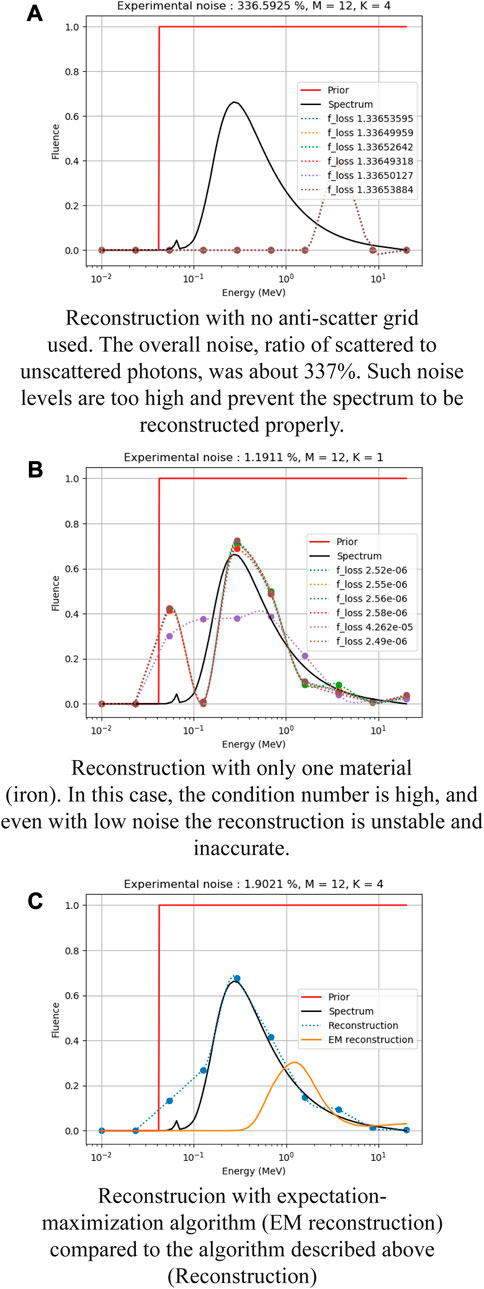
FIGURE 8. Ablation study of the spectrum reconstruction in nominal configuration: prior (solid red), source spectrum (solid black) and reconstructions (dotted lines).

More precisely, reconstructions have been performed independently in the nominal configuration in the cases where:

• No anti-scatter grid was used for the measurements (Figure 8A)

• Only one material (iron) was used for the experimental slabs (Figure 8B)

• The expectation-maximization (EM) algorithm was used for the reconstruction instead of the algorithm proposed in this study (Figure 8C)

4 Discussion

4.1 Impact of multiple materials

The work done in [10] led to a great reduction in orders of magnitude of the forward matrix condition number, and highlighted an exponential distribution of thicknesses for the optimal measurement set using one material. Results shown in Section 3.1 illustrate the impact of using multiple materials on the condition number, with two distinct cases.

Using multiple piled up materials is beneficial in comparison to the previous setup from [10]. This can be explained by the much larger size of the research space when multiple materials are allowed, leading to a better optimum than the single material algorithm. However, as shown in Figure 5A, the expected drawback of this larger research space is a worse stability. The reduction of the research space size thus plays a key role in the stability improvement.

With the second version of our algorithm presented in 1, where only one material is allowed per measurement, an even greater improvement of results is observed with a highly reduced condition number and a good stability, shown in Figure 4C and Figure 5B. Even though the research space is smaller than in the previous version of the algorithm (which theoretically includes this one’s particular case), the relevant constraints put on the optimizer allow a more thorough exploration, leading to the discovery of a better optimum.

4.2 Reduction of scatter noise

Reduction of the measurement scatter noise has proven to be necessary when a challenging high-energy spectrum is reconstructed. Indeed, even though the ill-posedness of the inverse problem is reduced by the search of optimal measurement sets, the condition number remains significant enough to disturb the reconstruction when the measurement noise is too high.

As displayed in Figure 6A, when a naive simulation configuration is used (config. 1) the scatter noise tends to become as large as 100%, leading to measurements unusable for reconstruction.

When the measurement slabs are optimally distributed within the experimental circle (config. 2), Figure 6B shows a substantial reduction of scattering, with unscattered rays noised by an amount of 50%. This scatter noise is however still way too high for the inversion.

Lastly, when a thick lead anti-scatter grid is added behind the measurement slabs (config. 3), the scatter noise is reduced to a negligible amount of around 3% as shown in Figure 6C. The lead layer allows the absorption of almost every scattered ray and the detection of the unscattered rays that pass through material slabs parallel to its axis. The scatter noise obtained with this last configuration appears to be small enough for the measurements to be used to solve the inverse problem and reconstruct the spectrum.

4.3 Schiff spectrum reconstruction

4.3.1 Nominal configuration

As shown in Figure 7, the overall reconstruction accuracy is satisfying in the nominal configuration, but two areas can be distinguished. For high energy (E > 40 keV) there is no restriction as the constraint step function is set to unity, and the reconstruction shows great accuracy even for as few as 12 interpolation points. However, in the low energy range, the points are constrained to 0 and are thus not optimized. In practice, this is necessary because of the much lower contribution of low energies in the transmission measurements. Indeed, when dense materials are subjected to an X-ray beam of given spectrum, most of the low-energy photons are absorbed and are not detected at the end. The difficulty to reconstruct the low energy part of spectra is thus an intrinsic issue for the inverse problem at hand.

4.3.2 Ablation studies

Figure 8A emphasizes the substantial impact of the presence of an anti-scatter grid in the experimental setup on the reconstruction accuracy. When nothing is done to reduce the scattered rays, the measurements are very noisy, leading inevitably to an inaccurate reconstruction.

Similarly, the influence of using multiple materials is illustrated in Figure 8B. Because only iron is allowed in the first optimization problem, the genetic algorithm cannot converge to a satisfying minimum of the condition number of the system. Thus, even with low noise, the reconstruction is unstable and inaccurate.

Finally, the interest of using the “trust-constr” algorithm for the second optimization problem formulated above is clearly highlighted in Figure 8C. When the expectation-maximization algorithm is used instead, as it has usually been done in other studies [10], the quality of the reconstruction is very poor for low and medium energy ranges, and the spectrum peak is not retrieved at the expected energy level.

5 Conclusion

In this article, a full spectrum reconstruction pipeline for high-energy X-ray sources was presented. Building on prior work which introduced the optimization of transmission measurements, the present work generalizes this approach to multiple calibration materials, enabling to reach better performance than thickness-only optimization. This work also demonstrated the importance of noise reduction to perform spectrum reconstruction in realistic experimental setups. As such, it showed that the design of an adapted anti-scatter grid is a precious asset to solve the inverse problem and obtain faithful spectrum estimations. Finally, a novel noise-robust reconstruction method was shown to outperform common expectation-maximization approaches, enabling a precise choice of spectrum resolution and a controlled injection of prior knowledge of the X-ray spectrum.

Data availability statement

The original contributions presented in the study are included in the article/Supplementary Material, further inquiries can be directed to the corresponding author.

Author contributions

KG and AF lead the research. AW wrote the code and conducted numerical experiments. AW, KG, and AF wrote the article. All authors contributed to the article and approved the submitted version.

Funding

The author(s) declare that no financial support was received for the research, authorship, and/or publication of this article.

Conflict of interest

The authors declare that the research was conducted in the absence of any commercial or financial relationships that could be construed as a potential conflict of interest.

Publisher’s note

All claims expressed in this article are solely those of the authors and do not necessarily represent those of their affiliated organizations, or those of the publisher, the editors and the reviewers. Any product that may be evaluated in this article, or claim that may be made by its manufacturer, is not guaranteed or endorsed by the publisher.

References

1. Sidky EY, Yu L, Pan X. Application of expectation maximization to x-ray spectrum estimation for medical accelerators from transmission data. San Diego, CA: SPIE Digital Library (2004). p. 856. doi:10.1117/12.535989

CrossRef Full Text | Google Scholar

2. Duan X, Wang J, Yu L, Leng S, McCollough CH. CT scanner x-ray spectrum estimation from transmission measurements. Med Phys (2011) 38:993–7. doi:10.1118/1.3547718

PubMed Abstract | CrossRef Full Text | Google Scholar

3. Wood WM. Shot-by-shot spectrum model for rod-pinch, pulsed radiography machines. AIP Adv (2018) 8:025105. doi:10.1063/1.5016299

CrossRef Full Text | Google Scholar

4. Waggener RG, Blough MM, Terry JA, Chen D, Lee NE, Zhang S, et al. X-ray spectra estimation using attenuation measurements from 25 kVp to 18 MV. Med Phys (1999) 26:1269–78. doi:10.1118/1.598622

PubMed Abstract | CrossRef Full Text | Google Scholar

5. Armbruster B, Hamilton RJ, Kuehl AK. Spectrum reconstruction from dose measurements as a linear inverse problem. Phys Med Biol (2004) 49:5087–99. doi:10.1088/0031-9155/49/22/005

PubMed Abstract | CrossRef Full Text | Google Scholar

6. Paniak LD, Charland PM. Enhanced bremsstrahlung spectrum reconstruction from depth–dose gradients. Phys Med Biol (2005) 50:3245–61. doi:10.1088/0031-9155/50/14/004

PubMed Abstract | CrossRef Full Text | Google Scholar

7. Sidky EY, Yu L, Pan X, Zou Y, Vannier M. A robust method of x-ray source spectrum estimation from transmission measurements: Demonstrated on computer simulated, scatter-free transmission data. J Appl Phys (2005) 97. doi:10.1063/1.1928312

CrossRef Full Text | Google Scholar

8. Zhao W, Niu K, Schafer S, Royalty K. An indirect transmission measurement-based spectrum estimation method for computed tomography. Phys Med Biol (2015) 60:339–57. doi:10.1088/0031-9155/60/1/339

PubMed Abstract | CrossRef Full Text | Google Scholar

9. FitzGerald P, Araujo S, Wu M, De Man B. Semiempirical, parameterized spectrum estimation for x-ray computed tomography. Med Phys (2021) 48:2199–213. doi:10.1002/mp.14715

PubMed Abstract | CrossRef Full Text | Google Scholar

10. Li M, Fan F-L, Cong W, Wang G. EM estimation of the X-ray spectrum with a genetically optimized step-wedge phantom. Front Phys (2021) 9:678171. doi:10.3389/fphy.2021.678171

CrossRef Full Text | Google Scholar

11. Schiff LI. Energy-angle distribution of thin target bremsstrahlung. Phys Rev (1951) 83:252–3. doi:10.1103/PhysRev.83.252

CrossRef Full Text | Google Scholar

12. Estre N, Eck D, Pettier J-L, Payan E, Roure C, Simon E. High-energy X-ray imaging applied to non destructive characterization of large nuclear waste drums. In: 2013 3rd International Conference on Advancements in Nuclear Instrumentation, Measurement Methods and their Applications (ANIMMA); 23-27 June 2013; Marseille, France (2013). 1–6. doi:10.1109/ANIMMA.2013.6727987

CrossRef Full Text | Google Scholar

13. Hubbell JH, Seltzer SM. Tables of X-ray mass attenuation coefficients and mass energy-absorption coefficients from 1 keV to 20 MeV for elements Z = 1 to 92 and 48 additional substances of dosimetric interest (2004). Available at: https://www.nist.gov/pml/x-ray-mass-attenuation-coefficients. doi:10.18434/T4D01F

CrossRef Full Text | Google Scholar

14. Storn R, Price K. Differential evolution–a simple and efficient heuristic for global optimization over continuous spaces. J Glob optimization (1997) 11:341–59. doi:10.1023/a:1008202821328

CrossRef Full Text | Google Scholar

15. Akima H. A new method of interpolation and smooth curve fitting based on local procedures. J ACM (JACM) (1970) 17:589–602. doi:10.1145/321607.321609

CrossRef Full Text | Google Scholar

16. Conn AR, Gould NI, Toint PL. Trust region methods (SIAM). Numer Optimization (2000) 2000:66.

Google Scholar