Planarity in cubic intuitionistic graphs and their application to control air traffic on a runway

Fuzzy modeling plays a pivotal role in various fields, including science, engineering, and medicine. In comparison to conventional models, fuzzy models offer enhanced accuracy, adaptability, and resemblance to real-world systems and help researchers to always make the best choice in complex problems. A type of fuzzy graph that is widely used in medical and psychological sciences is the cubic intuitionistic fuzzy graph, which plays an important role in various fields such as computer science, psychology, medicine, and political sciences. It is also used to find effective people in an organization or social institution. In this research endeavor, we embark upon elucidating the innovative notion of a cubic intuitionistic planar graph, delving into its intricate properties and attributes. Additionally, we unveil the novel concept of a cubic intuitionistic dual graph, thus enriching the realm of graph theory with further profundity. Furthermore, our exploration encompasses the elucidation of other pertinent terminologies, such as cubic intuitionistic multi-graphs, along with the categorization of edges into the distinct classifications of strong and weak edges. Moreover, we discern the concept of the degree of planarity within the context of CIPG and unveil the notion of strong and weak faces. Additionally, we delve into the construction of cubic intuitionistic dual graphs, which can be realized in cases where the initial graph is planar or possesses a degree of planarity $\ge 0.67$. Notably, we furnish the exposition with a comprehensive discussion on noteworthy findings and substantial results pertaining to these captivating topics, contributing valuable insights on the field of graph theory. Last, we shall endeavor to exemplify the practical relevance and importance of our research by presenting an illuminating real-world application, thus demonstrating the tangible impact and significance of our endeavors in this research article.

1 Introduction

Graph theory has significantly grown in importance as a field of study due to its widespread applications. The significance of graph theory has escalated, owing to its versatile uses. For instance, it plays a crucial role in calculating the shortest path between two nodes in services like Google Maps. Graph theory finds applications in various domains, such as computer networks, image processing, electric circuits, and road networks. For applications of graph theory in chemistry, refer to [1–4].

In certain graph networks, intersections between edges give rise to problems, such as planning issues for electrical circuits, metros, and utility corridors. The elimination of crossings between electric wires might be feasible, but avoiding such crossings in a road network is often more complex. In road networks, nodes represent specific locations and edges symbolize highways. Hence, it becomes critical to determine the necessity of road crossings. The solution of this problem may involve the construction of underpasses or flyovers, but this may result in higher costs. However, this approach effectively resolves numerous issues, including road accidents and traffic jams that arise in congested areas. It is important to note that the term “congested” is a linguistic expression without precise boundaries. Various degrees of congestion, such as “very highly congested,” “very congested,” “congested,” “low congested,” and “very low congested,” can be employed. Additionally, these linguistic terms are associated with membership values, allowing for a more nuanced representation of congestion levels.

Strong and weak routes are distinguished by their congestion levels, with strong routes being congested and weak routes remaining non-congested. When developing a city road network, intersections between two weak routes hold significance, while intersections between two strong routes can be inconvenient. These problems can be effectively addressed using a fuzzy planar graph. In 1964, Zadeh [5] recognized the lack of clarity and ambiguity in real-world problems, leading to the introduction of fuzzy sets. This advancement has transformed the landscape of science and technology, especially when dealing with partial information or inaccessible data, leading to the emergence of fuzzy theories.

The concept of fuzzy graph theory was introduced by Rosenfeld [6], marking the beginning of fuzzy research. Kaufmann [7] introduced the theory of fuzzy graphs (FGs) based on fuzzy relations. Mordeson and Nair [8] introduced the FG complement and its associated operations. Shannon and Atanassov [9] introduced the intuitionistic fuzzy relation (IFR) and intuitionistic fuzzy graph (IFG) as its foundation. Parvathi et al. [10] introduced various operations on IFGs, such as union and join. The study of intuitionistic fuzzy cycles related to IFGs was conducted in [11]. Jabbar et al. [12] introduced the concept of fuzzy dual graphs, while Samanta and Pal [13] introduced fuzzy planar graphs. Alshehri and Akram [14], and Akram et al. [15] introduced intuitionistic and Pythagorean fuzzy planar graphs. Nirmal and Dhanabal [16] discussed specific fuzzy planar graphs in non-deterministic polynomial time. Pal et al. [17] examined planarity in FGs and proposed an alternative approach without restricting edge crossings. For various applications of fuzzy graphs, refer to [18–35].

Zadeh [36] presented interval-valued fuzzy sets (IVFS) as extension of fuzzy sets. Akram and Dudek [37] described the basic concepts of the interval-valued fuzzy graph (IVFG). These IVFGs were further studied in [38]. The notion of the IVFG is perhaps more generalized and flexible than a fuzzy graph because the membership degrees of vertices and edges are in the form of intervals. The interval-valued intuitionistic fuzzy graphs were discussed in [39]. In [40], interval-valued intuitionistic fuzzy competition graphs are investigated. Pramanik et al. [41] proposed interval-valued planar graphs. On the other hand, the cubic set proposed by Jun et al. [42] is a blending of ideas of IVFS and a fuzzy set. During recent 5 years, a lot of research work has been performed in the domain of the cubic set. Rashid et al. [43] presented the basic theory of cubic graphs. Khan et al. [44] investigated cubic intuitionistic FGs. The cubic planar graphs have been studied by Muhiuddin et al. [45]. They also applied the planarity of cubic graphs in a road network problem. In [46], the cubic Pythagorean FGs were investigated. The vertex regularity for cubic fuzzy graph structures is investigated in [47].

1.1 Motivation

Cubic sets serve as a primary motivation for this study as they can effectively handle two types of processes simultaneously: one continuous and the other specific. Although a discrete process may demonstrate a present value, a continuous process can provide future or past estimates. Previous research has extensively explored cubic sets, but there has been relatively less focus on cubic graphs. In this study, we aim to integrate the planarity of both graphs, namely, IVFG and FG, into a single structure. The concept of a cubic planar graph also serves as a motivating factor for our research.

The following work on cubic intuitionistic planar graphs is discussed and coordinated as follows:

Section 2 provides several basic terms related to CIMS and CIMG. The concepts of strong and weak edges are defined for cubic intuitionistic graphs. Section 3 discusses the planarity of CIPG and other essential results. We define strong and weak faces and use them to define the cubic intuitionistic dual graph of a CIPG. Section 5 contains an application of a CIPG related to an airline route system. We also compare our result with cubic planar graphs.

2 Preliminaries

Definition 2.1. [5, 7]. Consider a non-empty set $\mathfrak{S}$ and the mapping $\mathfrak{J}:\mathfrak{S}\to [\mathrm{0,1}]$. Subsequently, a fuzzy set can be defined as

$\mathbb{Q}=\left\{\left(f,\mathfrak{J}\left(f\right)\right):f\in \mathfrak{S}\right\}.$

In addition, with a mapping $\mathfrak{H}:\mathfrak{S}\times \mathfrak{S}\to [\mathrm{0,1}]$, a fuzzy relation is defined as

$\mathbb{W}=\left\{⟨\left(f,t\right),\mathfrak{H}\left(f,t\right)⟩:f,t\in \mathfrak{S}\right\}.$

A pair $\mathbb{G}=(\mathbb{Q},\mathbb{W})$ is a fuzzy graph where a fuzzy set is denoted by $\mathbb{Q}$ and a fuzzy relation is denoted by $\mathbb{W}$ on $\mathfrak{S}$ such that

$\mathfrak{H}\left(f,t\right)\le \min \left\{\mathfrak{J}\left(f\right),\mathfrak{J}\left(t\right)\right\},$

for all $f,t\in \mathfrak{S}$, where $\mathfrak{H}(f,t)$ and $\mathfrak{J}(f)$ indicate the edge (f, t) membership value and the vertex f membership value, respectively. If a graph’s vertex f does not have any loops, then $\mathfrak{H}(f,f)=0$ and a graph with a loop at the vertex f, then $\mathfrak{H}(f,f)\ne 0$.

Definition 2.2. [48]. Consider a non-empty set $\mathfrak{S}$ and the mapping $\mathfrak{J}:\mathfrak{S}\to [\mathrm{0,1}]$. Subsequently, a fuzzy multi-set is defined over $\mathfrak{S}$ as $\mathbb{R}=\{f,{\mathfrak{J}}_p(f):f\in \mathfrak{S}\}$, for all p = 0, 1, 2, … , q_f, where $q_f=\max \{p:{\mathfrak{J}}_p\ne 0\}$.Taking a non-empty set $\mathfrak{S}$ along with the mapping $\mathfrak{J}:\mathfrak{S}\to [\mathrm{0,1}]$, $\mathfrak{H}:\mathfrak{S}\times \mathfrak{S}\to [\mathrm{0,1}]$. A fuzzy multi graph is defined as

$\mathbb{G}=\left\{⟨\left(f,t\right),{\mathfrak{H}}_p\left(f,t\right),p=\mathrm{1,2},\dots ,q_{ft}:\left(f,t\right)\in \mathfrak{S}\times \mathfrak{S}⟩\right\},$

such that ${\mathfrak{H}}_p(f,t)\le \min \{\mathfrak{J}(f),\mathfrak{J}(t)\}$, where $q_{ft}=\max \{(f,t):{\mathfrak{H}}_p(f,t)\ne 0\}$ and ${\mathfrak{H}}_p(f,t)$ and $\mathfrak{J}(f)$ indicate, respectively, the membership value of the fuzzy multi-edge and fuzzy vertex.

Definition 2.3. [49]. Consider a mapping ${\mathfrak{J}}^{+}:\mathfrak{S}\to [\mathrm{0,1}]$ and ${\mathfrak{J}}^{-}:\mathfrak{S}\to [\mathrm{0,1}]$. Following that, an interval-valued fuzzy set (IVFS) is defined as

${\mathbb{T}}^{\prime }=\left\{\left[{\mathfrak{J}}^{-}\left(f\right),{\mathfrak{J}}^{+}\left(f\right)\right]:f\in \mathfrak{S}\right\},$

where $0\le {\mathfrak{J}}^{-}\le {\mathfrak{J}}^{+}\le 1$. The IVFG is described by $\mathbb{G}=({\mathbb{T}}^{\prime },{\mathbb{Y}}^{\prime })$ such that ${\mathbb{T}}^{\prime }$ is an IVFS on $\mathfrak{S}$ and ${\mathbb{Y}}^{\prime }$ is on $\mathfrak{S}\times \mathfrak{S}$, satisfying

$\begin{array}{ccc}\hfill {\mathfrak{H}}^{-}\left(f,t\right)& \le \hfill & \min \left\{{\mathfrak{J}}^{-}\left(f\right),{\mathfrak{J}}^{-}\left(t\right)\right\},\hfill \\ \hfill {\mathfrak{H}}^{+}\left(f,t\right)& \le \hfill & \min \left\{{\mathfrak{J}}^{+}\left(f\right),{\mathfrak{J}}^{+}\left(t\right)\right\},\hfill \end{array}$

for all $f,t\in \mathfrak{S}$.Let ${\mathfrak{J}}_p^{+}:\mathfrak{S}\to [\mathrm{0,1}]$ and ${\mathfrak{J}}_p^{-}:\mathfrak{S}\to [\mathrm{0,1}]$ be the mappings such that ${\mathfrak{J}}_p^{-}\le {\mathfrak{J}}_p^{+}\forall f\in \mathfrak{S}$ and $p=\mathrm{0,1},\dots ,{\dot{q}}_f$, where ${\dot{q}}_f=\max \{p,\mathfrak{J}(f)\ne 0\}$. IVFMS, or the interval-valued fuzzy multiset, on $\mathfrak{S}$ can be defined as

$\mathbb{T}=\left(\mathfrak{S},\left[{\mathfrak{J}}_p^{-},{\mathfrak{J}}_p^{+}\right]\right)=\left\{f,\left[{\mathfrak{J}}_p^{-},{\mathfrak{J}}_p^{+}\right]|f\in \mathfrak{S},p=\mathrm{0,1},\dots ,{\dot{q}}_f\right\}.(1)$

Consider the mappings ${\mathfrak{H}}_v^{-}:\mathfrak{S}\times \mathfrak{S}\to [\mathrm{0,1}]$ and ${\mathfrak{H}}_v^{+}:\mathfrak{S}\times \mathfrak{S}\to [\mathrm{0,1}]$. Subsequently, the interval-valued fuzzy multi graph (IVFMG) on $\mathfrak{S}\times \mathfrak{S}$ is described by $(\mathbb{T},\mathbb{U})$ such that $\mathbb{T}$ provided in (1) and $\mathbb{U}$ are given as follows:

$\mathbb{U}=\left(\mathfrak{S}\times \mathfrak{S},\left[{\mathfrak{H}}_v^{-},{\mathfrak{H}}_v^{+}\right],v=\mathrm{0,1},\dots ,{\dot{q}}_f\right\},$

such that ${\mathfrak{H}}_v^{-}(f,t)\le \min \{{\mathfrak{J}}_p^{-}(f),{\mathfrak{J}}_p^{-}(t)\}$ and ${\mathfrak{H}}_v^{+}(f,t)\le \min \{{\mathfrak{J}}_p^{+}(f),{\mathfrak{J}}_p^{+}(t)\}$, where p = 0, 1, 2, … , q_f, v = 0, 1, 2, … , q_f, $q_f=\max \{p:{\mathfrak{J}}_p\ne 0\}$, and $q_{ft}=\max \{(f,t):{\mathfrak{H}}_v(f,t)\ne 0\}$.

Definition 2.4. A cubic multi-set is a combination of IVFMS and FMS expressed as

$\mathbb{O}=\left\{⟨\left[{\mathfrak{J}}_p^{-},{\mathfrak{J}}_p^{+}\right],{\mathfrak{J}}_p^{*}⟩|p=\mathrm{0,1},\dots ,{\dot{q}}_f\right\},$

where ${\dot{q}}_f=\max \{p,\mathfrak{J}(f)\ne 0\}$.

Definition 2.5. [50]. Take the mappings $\mathfrak{J}:\mathfrak{S}\to [\mathrm{0,1}]$ and $\mathfrak{A}:\mathfrak{S}\to [\mathrm{0,1}]$ to define the intuitionistic fuzzy set (IFS) as

$\mathbb{B}=\left\{f,\mathfrak{J}\left(f\right),\mathfrak{A}\left(f\right)|f\in \mathfrak{S}\right\},$

where $\mathfrak{J}(f)$ and $\mathfrak{A}(f)$ are the membership value and non-membership value, respectively, satisfying $\mathfrak{J}(f)+\mathfrak{A}(f)\le 1$. In the universe of discourse, an intuitionistic fuzzy relation (IFR) $\mathfrak{S}\times \mathfrak{S}$ along with the mappings $\mathfrak{H}:\mathfrak{S}\times \mathfrak{S}\to [\mathrm{0,1}]$ and $\mathfrak{L}:\mathfrak{S}\times \mathfrak{S}\to [\mathrm{0,1}]$ is also described as an IFS, which is

$\mathbb{P}=\left\{\left(f,t\right),\mathfrak{H}\left(f,t\right),\mathfrak{L}\left(f,t\right)|\left(f,t\right)\in \mathfrak{S}\times \mathfrak{S}\right\},$

along with $\mathfrak{H}(f,t)+\mathfrak{L}(f,t)\le 1$. Consider a graph $\mathbb{G}$ with a pair of IFS and IFR, i.e., $\mathbb{G}=(\mathbb{B},\mathbb{P})$. Then, $\mathbb{G}$ is known as intuitionistic FG if the following conditions hold:

$\mathfrak{H}\left(f,t\right)\le \min \left\{\mathfrak{J}\left(t\right),\mathfrak{J}\left(t\right)\right\}$

and

$\mathfrak{L}\left(f,t\right)\le \max \left\{\mathfrak{A}\left(t\right),\mathfrak{A}\left(t\right)\right\},$

such that $0\le \mathfrak{H}(f,t)+\mathfrak{L}(f,t)\le 1$.

Definition 2.6. A count membership function and a count non-membership function define an intuitionistic fuzzy multi-set (IFMS) and is described as $C{M}_{\mathbb{B}}:\mathfrak{S}\to \mathbb{Q}$ and $C{N}_{\mathbb{B}}:\mathfrak{S}\to \mathbb{Q}$, where $\mathbb{B}$ is a function and a crisp multiset chosen from [0,1] is $\mathbb{Q}$. If $f\in \mathfrak{S}$ then $C{M}_{\mathbb{B}}(t)$ and $C{N}_{\mathbb{B}}(t)$ are the crisp multisets. Additionally, the sequence of the membership is specified in the descending order, although the non-membership sequence may not be in that order. The IFMS is described as

${\mathbb{I}}^{\prime }=\left\{t,{\mathfrak{J}}^a\left(t\right),{\mathfrak{A}}^a\left(t\right)|t\in \mathfrak{S}\right\},$

where a = 1, 2, … , q_t and $q_t=\max \{a:{\mathfrak{J}}^a\ne 0\}$.

Definition 2.7. [51]. Consider the mappings ${\mathfrak{J}}^{-}:\mathfrak{S}\to [\mathrm{0,1}]$, ${\mathfrak{J}}^{+}:\mathfrak{S}\to [\mathrm{0,1}]$, ${\mathfrak{A}}^{+}:\mathfrak{S}\to [\mathrm{0,1}]$, and ${\mathfrak{A}}^{-}:\mathfrak{S}\to [\mathrm{0,1}]$. A definition of the interval-valued intuitionistic fuzzy set (IVIFS) is given as

$\mathbb{V}=\left\{\left(f,t\right),\left[{\mathfrak{J}}^{-},{\mathfrak{J}}^{+}\right],\left[{\mathfrak{A}}^{-},{\mathfrak{A}}^{+}\right]:\left(f,t\right)\in \mathfrak{S}\right\}$

such that $0\le [{\mathfrak{J}}^{-},{\mathfrak{J}}^{+}]+[{\mathfrak{A}}^{-},{\mathfrak{A}}^{+}]\le 1$, which is observable as $0\le {\mathfrak{J}}^{-}+{\mathfrak{A}}^{-}\le 1$ and $0\le {\mathfrak{J}}^{+}+{\mathfrak{A}}^{+}\le 1$. Similarly, the interval-valued intuitionistic fuzzy relation (IVIFR) is expressed as

$\mathbb{D}=\left\{\left(f,t\right),\left[{\mathfrak{H}}^{-},{\mathfrak{H}}^{+}\right],\left[{\mathfrak{L}}^{-},{\mathfrak{L}}^{+}\right]:\left(f,t\right)\in \mathfrak{S}\times \mathfrak{S}\right\}$

along with the mappings ${\mathfrak{H}}^{-}:\mathfrak{S}\times \mathfrak{S}\to [\mathrm{0,1}]$, ${\mathfrak{H}}^{+}:\mathfrak{S}\times \mathfrak{S}\to [\mathrm{0,1}]$, ${\mathfrak{L}}^{+}:\mathfrak{S}\times \mathfrak{S}\to [\mathrm{0,1}]$, and ${\mathfrak{L}}^{-}:\mathfrak{S}\times \mathfrak{S}\to [\mathrm{0,1}]$, fulfilling the requirements $0\le [{\mathfrak{H}}^{-},{\mathfrak{H}}^{+}]+[{\mathfrak{L}}^{-},{\mathfrak{L}}^{+}]\le 1$. Take a graph $\mathbb{G}$ with pairs of IVIFS and IVIFR such as $\mathbb{G}=(\mathbb{V},\mathbb{D})$, then $\mathbb{G}$ is referred to as an intuitionistic interval-valued fuzzy graph (IIVFG) if it met the following criteria:

${\mathfrak{H}}^{-}\left(f,t\right)\le \min \left\{{\mathfrak{J}}^{-}\left(f\right),{\mathfrak{J}}^{-}\left(t\right)\right\},$

${\mathfrak{H}}^{+}\left(f,t\right)\le \min \left\{{\mathfrak{J}}^{+}\left(f\right),{\mathfrak{J}}^{+}\left(t\right)\right\},$

${\mathfrak{L}}^{-}\left(f,t\right)\le \max \left\{{\mathfrak{A}}^{-}\left(f\right),{\mathfrak{A}}^{-}\left(t\right)\right\},$

${\mathfrak{L}}^{+}\left(f,t\right)\le \max \left\{{\mathfrak{A}}^{+}\left(f\right),{\mathfrak{A}}^{+}\left(t\right)\right\},$

for all $f,t\in \mathfrak{S}$.

Definition 2.8. A count membership function $C{M}_H:\mathfrak{S}\to \mathbb{Q}$ and count non-membership function $C{N}_H:\mathfrak{S}\to \mathbb{Q}$ defined an intuitionistic interval-valued fuzzy multi-set (IIVFMS), and $\mathbb{Q}$ denotes the crisp  multiset obtained from [0,1]. If $(f,t)\in \mathfrak{S}$, then CM_H(f, t) and CN_H(f, t) are the crisp multisets. Additionally, the non-membership sequence is not necessarily in the decreasing order, while the membership sequence  is defined in the decreasing order. The IVIFMS can also be described as

$\mathbb{H}=\left\{\left(f,t\right),{\mathfrak{J}}^a\left(f,t\right),{\mathfrak{A}}^a\left(f,t\right)|\left(f,t\right)\in \mathfrak{S}\right\},$

where a = 1, 2, … , q_p and $q_p=\max \{a:{\mathfrak{J}}^a\ne 0\}$.

3 Cubic intuitionistic planar graph

Definition 3.1. [44]. A graph that contains both IFS and IVIFS, as defined by the cubic intuitionistic fuzzy set (CIFS):

$\mathbb{C}=\left\{f,\mathbb{V},\mathbb{B}:f\in \mathfrak{S}\right\},$

where IVIFS is $\mathbb{V}$ and IFS is $\mathbb{B}$.Now a cubic intuitionistic fuzzy graph is a pair $\mathbb{G}=(\mathbb{V},\mathbb{B})$ of the crisp graph ${\mathbb{G}}^{*}=(\mathfrak{S},\mathbb{E})$, where $\mathbb{V}=\{f,⟨([{\mathfrak{J}}^{-},{\mathfrak{J}}^{+}],[{\mathfrak{A}}^{-},{\mathfrak{A}}^{+}]),({\mathfrak{J}}^{*},{\mathfrak{A}}^{*})⟩:f\in \mathfrak{S}\}$ is a cubic intuitionistic fuzzy set and

$\mathbb{B}=\left\{\left(f,t\right),⟨\left(\left[{\mathfrak{H}}^{-},{\mathfrak{H}}^{+}\right],\left[{\mathfrak{L}}^{-},{\mathfrak{L}}^{+}\right]\right),\left({\mathfrak{H}}^{*},{\mathfrak{L}}^{*}\right)⟩:\left(f,t\right)\in \mathfrak{S}\times \mathfrak{S}\right\}$

is a cubic intuitionistic fuzzy relation on $\mathfrak{S}\times \mathfrak{S}$, satisfying the following conditions:

${\mathfrak{H}}^{-}\left(f,t\right)\le \min \left\{{\mathfrak{J}}^{-}\left(f\right),{\mathfrak{J}}^{-}\left(t\right)\right\},$

${\mathfrak{H}}^{+}\left(f,t\right)\le \min \left\{{\mathfrak{J}}^{+}\left(f\right),{\mathfrak{J}}^{+}\left(t\right)\right\},$

${\mathfrak{L}}^{-}\left(f,t\right)\le \max \left\{{\mathfrak{A}}^{-}\left(f\right),{\mathfrak{A}}^{-}\left(t\right)\right\},$

${\mathfrak{L}}^{+}\left(f,t\right)\le \max \left\{{\mathfrak{A}}^{+}\left(f\right),{\mathfrak{A}}^{+}\left(t\right)\right\},$

${\mathfrak{H}}^{*}\left(f,t\right)\le \min \left\{{\mathfrak{J}}^{*}\left(t\right),{\mathfrak{J}}^{*}\left(t\right)\right\},$

${\mathfrak{L}}^{*}\left(f,t\right)\le \max \left\{{\mathfrak{A}}^{*}\left(t\right),{\mathfrak{A}}^{*}\left(t\right)\right\},$

and $0\le [{\mathfrak{J}}^{-},{\mathfrak{J}}^{+}]+[{\mathfrak{A}}^{-},{\mathfrak{A}}^{+}]\le 1$, $0\le [{\mathfrak{H}}^{-},{\mathfrak{H}}^{+}]+[{\mathfrak{L}}^{-},{\mathfrak{L}}^{+}]\le 1$, $0\le {\mathfrak{J}}^{*}+{\mathfrak{A}}^{*}\le 1$, and $0\le {\mathfrak{H}}^{*}+{\mathfrak{L}}^{*}\le 1$ along with the mappings ${\mathfrak{H}}^{-}:\mathfrak{S}\times \mathfrak{S}\to [\mathrm{0,1}]$, ${\mathfrak{H}}^{+}:\mathfrak{S}\times \mathfrak{S}\to [\mathrm{0,1}]$, ${\mathfrak{L}}^{+}:\mathfrak{S}\times \mathfrak{S}\to [\mathrm{0,1}]$, ${\mathfrak{L}}^{-}:\mathfrak{S}\times \mathfrak{S}\to [\mathrm{0,1}]$, ${\mathfrak{J}}^{-}:\mathfrak{S}\to [\mathrm{0,1}]$, ${\mathfrak{J}}^{+}:\mathfrak{S}\to [\mathrm{0,1}]$, ${\mathfrak{A}}^{+}:\mathfrak{S}\to [\mathrm{0,1}]$, ${\mathfrak{A}}^{-}:\mathfrak{S}\to [\mathrm{0,1}]$, ${\mathfrak{J}}^{*}:\mathfrak{S}\to [\mathrm{0,1}]$, and ${\mathfrak{A}}^{*}:\mathfrak{S}\to [\mathrm{0,1}]$.

Definition 3.2. IVIFMS $(\mathbb{H})$ and IFMS $({\mathbb{I}}^{\prime })$ as a pair forms the intuitionistic cubic multiset $\mathbb{C}$ that is ${\mathbb{C}}_{\mathbb{B}}=(\mathbb{H},{\mathbb{I}}^{\prime })$. Similarly, an intuitionistic cubic multi graph is $\mathbb{G}=(\mathbb{V},\mathbb{B})$ on the crisp graph ${\mathbb{G}}^{*}=({\mathfrak{S}}^{*},{\mathbb{E}}^{*})$, where $\mathbb{V}=\{f,⟨([{\mathfrak{J}}_p^{-},{\mathfrak{J}}_p^{+}],[{\mathfrak{A}}_p^{-},{\mathfrak{A}}_p^{+}])({\mathfrak{J}}_p^{*},{\mathfrak{A}}_p^{*})⟩:f\in \mathfrak{S}\}$ is a cubic intuitionistic fuzzy set and $\mathbb{B}=\{(f,t),⟨([{\mathfrak{H}}_v^{-},{\mathfrak{H}}_v^{+}],[{\mathfrak{L}}_v^{-},{\mathfrak{L}}_v^{+}]),({\mathfrak{H}}_v^{*},{\mathfrak{L}}_v^{*})⟩:(f,t)\in \mathfrak{S}\times \mathfrak{S}\}$ is a cubic intuitionistic fuzzy relation on $\mathfrak{S}\times \mathfrak{S}$, satisfying the following conditions:

${\mathfrak{H}}_v^{-}\left(f,t\right)\le \min \left\{{\mathfrak{J}}_z^{-}\left(f\right),{\mathfrak{J}}_z^{-}\left(t\right)\right\},$

${\mathfrak{H}}_v^{+}\left(f,t\right)\le \min \left\{{\mathfrak{J}}_z^{+}\left(f\right),{\mathfrak{J}}_z^{+}\left(t\right)\right\},$

${\mathfrak{L}}_v^{-}\left(f,t\right)\le \max \left\{{\mathfrak{A}}_z^{-}\left(f\right),{\mathfrak{A}}_z^{-}\left(t\right)\right\},$

${\mathfrak{L}}_v^{+}\left(f,t\right)\le \max \left\{{\mathfrak{A}}_z^{+}\left(f\right),{\mathfrak{A}}_z^{+}\left(t\right)\right\},$

${\mathfrak{H}}_v^{*}\left(f,t\right)\le \min \left\{{\mathfrak{J}}_z^{*}\left(t\right),{\mathfrak{J}}_z^{*}\left(t\right)\right\},$

${\mathfrak{L}}_v^{*}\left(f,t\right)\le \max \left\{{\mathfrak{A}}_z^{*}\left(t\right),{\mathfrak{A}}_z^{*}\left(t\right)\right\},$

and $0\le [{\mathfrak{J}}_p^{-},{\mathfrak{J}}_p^{+}]+[{\mathfrak{A}}_p^{-},{\mathfrak{A}}_p^{+}]\le 1$, $0\le [{\mathfrak{H}}_v^{-},{\mathfrak{H}}_v^{+}]+[{\mathfrak{L}}_v^{-},{\mathfrak{L}}_v^{+}]\le 1$, $0\le {\mathfrak{J}}_p^{*}+{\mathfrak{A}}_p^{*}\le 1$, and $0\le {\mathfrak{H}}_v^{*}+{\mathfrak{A}}_{D_v}{D_v}^{*}\le 1$ along with the mappings ${\mathfrak{H}}_v^{-}:\mathfrak{S}\times \mathfrak{S}\to [\mathrm{0,1}]$, ${\mathfrak{H}}_v^{+}:\mathfrak{S}\times \mathfrak{S}\to [\mathrm{0,1}]$, ${\mathfrak{L}}_v^{+}:\mathfrak{S}\times \mathfrak{S}\to [\mathrm{0,1}]$, ${\mathfrak{L}}_v^{-}:\mathfrak{S}\times \mathfrak{S}\to [\mathrm{0,1}]$, ${\mathfrak{J}}_p^{-}:\mathfrak{S}\to [\mathrm{0,1}]$, ${\mathfrak{J}}_p^{+}:\mathfrak{S}\to [\mathrm{0,1}]$, ${\mathfrak{A}}_p^{+}:\mathfrak{S}\to [\mathrm{0,1}]$, ${\mathfrak{A}}_p^{-}:\mathfrak{S}\to [\mathrm{0,1}]$, ${\mathfrak{J}}_p^{*}:\mathfrak{S}\to [\mathrm{0,1}]$, and ${\mathfrak{A}}_p^{*}:\mathfrak{S}\to [\mathrm{0,1}]$, where p = 0, 1, 2, … , q_o, v = 0, 1, 2, … , q_f, $q_f=\max \{p:{\mathfrak{J}}_p\ne 0\},$ and $q_{ft}=\max \{(f,t):{\mathfrak{H}}_v(f,t)\ne 0\}$.

Example 3.3. Let $\mathfrak{S}=\{a,b,c\}$ and ${\mathfrak{J}}^{-}(a)=0.2,{\mathfrak{J}}^{+}(a)=0.4,{\mathfrak{J}}^{*}(a)=0.5,{\mathfrak{A}}^{-}(a)=0.3,{\mathfrak{A}}^{+}(a)=0.4,{\mathfrak{A}}^{*}(a)=0.2$. Next, for the vertex b, ${\mathfrak{J}}^{-}(b)=0.1,{\mathfrak{J}}^{+}(b)=0.5,{\mathfrak{J}}^{*}(b)=0.3,{\mathfrak{A}}^{-}(b)=0.4,{\mathfrak{A}}^{+}(a)=0.5,{\mathfrak{A}}^{*}(b)=0.4$, and for the vertex c, ${\mathfrak{J}}^{-}(c)=0.3,{\mathfrak{J}}^{+}(c)=0.4,{\mathfrak{J}}^{*}(c)=0.7,{\mathfrak{A}}^{-}(c)=0.4,{\mathfrak{A}}^{+}(c)=0.6,{\mathfrak{A}}^{*}(c)=0.3$. The vertices a and b have two edges between them, indicating that the graph is an ICMG. The values of the several edges are shown in Figure 1.

FIGURE 1

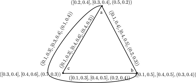
FIGURE 1. Example of an ICMG.

Definition 3.4. The strength of an edge for an ICMG $\mathbb{G}=(\mathbb{V},\mathbb{B})$ can be determined by using

$\begin{array}{ccc}\hfill I_{op}& =\hfill & \left({\mathrm{M}}_{\mathrm{𝔬}\mathrm{𝔭}},{\mathrm{N}}_{\mathrm{𝔬}\mathrm{𝔭}}\right)\hfill \\ \hfill & =\hfill & \langle \left[{{\mathrm{M}}_{\mathrm{𝔬}\mathrm{𝔭}}}^{-},{{\mathrm{M}}_{\mathrm{𝔬}\mathrm{𝔭}}}^{+}\right],\left[{\mathrm{N}}_{\mathrm{𝔬}\mathrm{𝔭}},{{\mathrm{N}}_{\mathrm{𝔬}\mathrm{𝔭}}}^{+}\right],\left({\mathrm{M}}_{\mathrm{𝔬}\mathrm{𝔭}},{{\mathrm{N}}_{\mathrm{𝔬}\mathrm{𝔭}}}^{*}\right)\rangle ,\hfill \\ \hfill & =\hfill & \langle \left[\frac{{\mathfrak{H}}_{op}^{-}}{\min \left({\mathfrak{J}}_o^{+},{\mathfrak{J}}_o^{+}\right)},\frac{{\mathfrak{H}}_{op}^{+}}{\min \left({\mathfrak{J}}_o^{+},{\mathfrak{J}}_o^{+}\right)}\right],\left[\frac{{\mathfrak{L}}_{op}^{-}}{\max \left({\mathfrak{A}}_o^{+},{\mathfrak{A}}_o^{+}\right)},\frac{{\mathfrak{L}}_{op}^{+}}{\max \left({\mathfrak{A}}_o^{+},{\mathfrak{A}}_o^{+}\right)}\right],\left(\frac{{\mathfrak{H}}_{op}^{*}}{\min \left({\mathfrak{J}}_o^{*},{\mathfrak{J}}_o^{*}\right)},\frac{{\mathfrak{L}}_{op}^{*}}{\max \left({\mathfrak{A}}_o^{*},{\mathfrak{A}}_o^{*}\right)}\right)\rangle ,\hfill \end{array}$

where the edge strength for the membership value is represented by ${\mathrm{M}}_{\mathrm{𝔬}\mathrm{𝔭}},$ and in the same manner, the edge strength of the non-membership value is represented by ${\mathrm{N}}_{\mathrm{𝔬}\mathrm{𝔭}}$. Intuitionistic strong cubic edges are described as such if ${\mathrm{M}}_{\mathrm{𝔬}\mathrm{𝔭}}\ge 0.5$ and ${\mathrm{N}}_{\mathrm{𝔬}\mathrm{𝔭}}\le 0.5$. If not, it is obviously a weak edge.

When using the ICMG, the intersection of two edges provides a specific value. This amount is known as a intuitionistic cubic-valued number. If two edges (l, k) and (e, r) cut each other at the point $\mathcal{P}$, then the intuitionistic cubic number at $\mathcal{P}$ is determined as

$I_{\mathcal{P}}=\left(M_{\mathcal{P}},N_{\mathcal{P}}\right)=\left(\frac{M_{lk}+M_{er}}{2},\frac{N_{lk}+N_{er}}{2}\right).$

A graph containing no cutting points between the edges is a planar graph. Planarity is affected by the number of cutting edges. If the number of cutting edges is greater, planarity is reduced, and vice versa. This motivates to introduce the concept of an intuitionistic cubic planar graph.

Definition 3.5. Suppose $\mathbb{G}=(\mathbb{V},\mathbb{B})$ is an ICMG along the cutting points ${\mathcal{P}}_1,{\mathcal{P}}_2,\dots ,{\mathcal{P}}_k$ and a specific graphical orientation, then the degree of planarity of planar graph $\mathbb{G}$ can be calculated as

$\mathfrak{F}=\left({\mathfrak{F}}_M,{\mathfrak{F}}_N\right)=⟨\left[{\mathfrak{F}}_M^{-},{\mathfrak{F}}_M^{+}\right]\left[{\mathfrak{F}}_N^{-},{\mathfrak{F}}_N^{+}\right]\left({\mathfrak{F}}_M^{*},{\mathfrak{F}}_N^{*}\right)⟩,$

where

$\begin{array}{ccc}\hfill {\mathfrak{F}}_M^{-}& =\hfill & \frac{1}{1+\left(M_{{\mathcal{P}}_1}^{+},M_{{\mathcal{P}}_2}^{+},\dots ,M_{{\mathcal{P}}_k}^{+}\right)},\hfill \\ \hfill {\mathfrak{F}}_M^{+}& =\hfill & \frac{1}{1+\left(M_{{\mathcal{P}}_1}^{-},M_{{\mathcal{P}}_2}^{-},\dots ,M_{{\mathcal{P}}_k}^{-}\right)},\hfill \\ \hfill {\mathfrak{F}}_M^{*}& =\hfill & \frac{1}{1+\left(M_{{\mathcal{P}}_1}^{*},M_{{\mathcal{P}}_2}^{*},\dots ,M_{{\mathcal{P}}_k}^{*}\right)},\hfill \\ \hfill {\mathfrak{F}}_N^{-}& =\hfill & \frac{1}{1+\left(N_{{\mathcal{P}}_1}^{+},N_{{\mathcal{P}}_2}^{+},\dots ,N_{{\mathcal{P}}_k}^{+}\right)},\hfill \\ \hfill {\mathfrak{F}}_N^{+}& =\hfill & \frac{1}{1+\left(N_{{\mathcal{P}}_1}^{-},N_{{\mathcal{P}}_2}^{-},\dots ,N_{{\mathcal{P}}_k}^{-}\right)},\hfill \\ \hfill {\mathfrak{F}}_N^{*}& =\hfill & \frac{1}{1+\left(N_{{\mathcal{P}}_1}^{*},N_{{\mathcal{P}}_2}^{*},\dots ,N_{{\mathcal{P}}_k}^{*}\right)}.\hfill \end{array}$

Here, we can observe $0\le {\mathfrak{F}}_M\le 1$ and $0\le {\mathfrak{F}}_N\le 1$.

A graph without any cutting point have a planarity value ⟨ [18][1, 1](1, 1)⟩. The cutting point between edges increases if ${\mathfrak{F}}_N$ decreases and ${\mathfrak{F}}_M$ increases and vice versa. Each ICMG having a certain planarity value is an intuitionistic cubic planar graph.

Example 3.6. Take $\mathbb{G}=(\mathbb{V},\mathbb{B})$ as a ICMG with a crisp graph ${\mathbb{G}}^{*}=(\mathfrak{S},\mathbb{E})$, where $\mathfrak{S}=\{l,k,e,r\}$ and $\mathbb{E}=\{lk,ke,er,rl\}$. The vertex and edge membership and non-membership are represented in Figure 2 and Table 1. Consider the cutting edge lr. Then, we compute

$M_{lr}^{-}=\frac{0.2}{\min \left(0.4,0.4\right)}=\frac{0.2}{0.4}=0.5,$

$M_{lr}^{+}=\frac{0.3}{\min \left(0.4,0.4\right)}=\frac{0.3}{0.4}=0.75,$

$M_{lr}^{*}=\frac{0.1}{\min \left(0.5,0.1\right)}=\frac{0.1}{0.1}=1,$

$N_{lr}^{-}=\frac{0.4}{\max \left(0.6,0.5\right)}=\frac{0.4}{0.6}=0.66,$

$N_{lr}^{+}=\frac{0.6}{\max \left(0.6,0.5\right)}=\frac{0.6}{0.6}=1,$

$N_{lr}^{*}=\frac{0.4}{\max \left(0.4,0.3\right)}=\frac{0.4}{0.4}=1.$

So, I_lr = ⟨[0.5, 0.75][0.66, 1](1, 1)⟩. By repeating the same technique for the edge (k, e), we obtain I_ke = ⟨[0.5, 1][0.5, 1](1, 1)⟩.

$M_{\mathcal{P}}=\left(\left[\frac{0.5+0.5}{2},\frac{1+0.75}{2}\right],\frac{1+1}{2}\right)=\left(\left[0.5,0.87\right],1\right).$

Similarly,

$N_{\mathcal{P}}=\left(\left[\frac{0.66+0.5}{2},\frac{1+1}{2}\right],\frac{1+1}{2}\right)=\left(\left[0.58,1\right],1\right),$

$I_{\mathcal{P}}=⟨\left[0.5,0.87\right],\left[0.58,1\right],\left(\mathrm{1,1}\right)⟩.$

Next, we evaluate the valueofplanarity as ${\mathfrak{F}}_M^{-}=\frac{1}{1+0.87}=0.53$, ${\mathfrak{F}}_M^{+}=\frac{1}{1+0.5}=0.66$,${\mathfrak{F}}_M^{*}=\frac{1}{1+1}=0.5$, ${\mathfrak{F}}_N^{-}=\frac{1}{1+1}=0.5$,${\mathfrak{F}}_N^{+}=\frac{1}{1+0.58}=0.63$,and ${\mathfrak{F}}_N^{*}=\frac{1}{1+1}=0.5$.$\mathfrak{F}=⟨[0.53,0.66],[0.5,0.63],(0.5,0.5)⟩$.

FIGURE 2

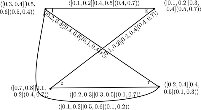
FIGURE 2. ICMG G=(S,I).

TABLE 1

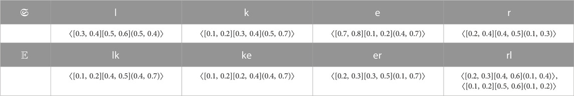
TABLE 1. Vertex and edge membership and non-membership.

Theorem 3.7. The value of planarity is ${\mathfrak{F}}_M=\frac{1}{1+n_{\mathcal{P}}}$, ${\mathfrak{F}}_N=\frac{1}{1+n_{\mathcal{P}}},$ and ${\mathfrak{F}}_M+{\mathfrak{F}}_N\le 1$ for a complete CIG, where the total number of cutting points between the edges is $n_{\mathcal{P}}$.

Strong cubic intuitionistic planar graphs (SCIPGs) are graphs that have a cubic planarity value of at least 0.5 for their membership parts, and the non-membership component is less than or equal to 0.5. Alternatively, we have $\mathfrak{F}=({\mathfrak{F}}_M,{\mathfrak{F}}_N)$, where ${\mathfrak{F}}_M\ge 0.5$ and ${\mathfrak{F}}_N\le 0.5$.

Theorem 3.8. The number of cutting points between the strong edges for SCIPG is at most 1.

Proof. Consider two cutting points ${\mathcal{P}}_1$ and ${\mathcal{P}}_2$ for cubic intuitionistic strong edges (o, p) and (f, t) along ${\mathrm{M}}_{\mathrm{𝔬}\mathrm{𝔭}}\ge 0.5$ and ${\mathrm{N}}_{\mathrm{𝔬}\mathrm{𝔭}}\le 0.5$ cubic intuitionistic planarity value. Then, we obtain, $\frac{{\mathrm{N}}_{\mathrm{𝔬}\mathrm{𝔭}}+N_{op}}{2}\le 0.5$ and $\frac{{\mathrm{M}}_{\mathrm{𝔬}\mathrm{𝔭}}+M_{op}}{2}\ge 0.5$, which implies that $1+N_{{\mathcal{P}}_1}+N_{{\mathcal{P}}_2}\le 2$ and $1+M_{{\mathcal{P}}_1}+M_{{\mathcal{P}}_2}\ge 2$, demonstrating that ${\mathfrak{F}}_N\ge 0.5$ and ${\mathfrak{F}}_M\le 0.5$. This implies that $\mathbb{G}$ is a SCIPG. Therefore, there can only be one cutting point among strong edges. Planarity decreases as the amount or number of cutting places between the strong cubic intuitionistic edges increases. The degree of planarity possessed by the SCIPG is ${\mathfrak{F}}_N\le 0.5$ and ${\mathfrak{F}}_M\ge 0.5$. The graph will be a planar graph if there is exactly one cutting point between any two edges and if there are no crossings between any two edges. Therefore, there can be precisely one cutting point between any two edges.

Theorem 3.9. Consider a CIPG $\mathbb{G}$ with the planarity value $\mathfrak{F}=({\mathfrak{F}}_M,{\mathfrak{F}}_N)$, where ${\mathfrak{F}}_N\le ⟨[0.33,0.33],0.33⟩$ and ${\mathfrak{F}}_M\ge ⟨[0.67,0.67],0.67⟩$. Therefore, none of the strong edges in $\mathbb{G}$ have a cutting point.

Proof. Now, we take a CIPG $\mathbb{G}$ with a planarity value $\mathfrak{F}=⟨[0.67,0.67],[0.33,0.33],(0.67,0.33)⟩$, and two strong cubic intuitionistic edges (l, k) (e, r) cut each other at $\mathbb{Q}$. As these are strong edges, so ${\mathrm{M}}_{\mathrm{𝔩}\mathrm{𝔨}}\ge 0.5$, ${\mathrm{N}}_{\mathrm{𝔩}\mathrm{𝔨}}\le 0.5$, M_er ≥ 0.5, and N_er ≤ 0.5. Now, by Theorem 3.7, the given value of $\mathfrak{F}$ is ${\mathfrak{F}}_N=\frac{1}{1+0.5}\ge 0.33$, and ${\mathfrak{F}}_M=\frac{1}{1+0.5}\le 0.67$ which are in opposition to the degree of planarity of strong edges because ${\mathfrak{F}}_N\ge 0.33$ and ${\mathfrak{F}}_M\ge 0.67$. Therefore, the cubic intuitionistic strong edges do not meet at a cutting point.

Definition 3.10. Consider a rational number 0 ≤ c ≤ 0.5 for a CIPG. Then, an edge (l, k) is an considerable edge if $⟨[\frac{{\mathfrak{H}}_{lk}^{-}}{\min ({\mathfrak{J}}_l^{+},{\mathfrak{J}}_l^{+})},\frac{{\mathfrak{H}}_{lk}^{+}}{\min ({\mathfrak{J}}_l^{+},{\mathfrak{J}}_l^{+})}],\frac{{\mathfrak{H}}_{lk}^{*}}{\min ({\mathfrak{J}}_l^{*},{\mathfrak{J}}_l^{*})}⟩\ge c$, $⟨[\frac{{\mathfrak{L}}_{lk}^{-}}{\max ({\mathfrak{A}}_l^{+},{\mathfrak{A}}_l^{+})},\frac{{\mathfrak{L}}_{lk}^{+}}{\max ({\mathfrak{A}}_l^{+},{\mathfrak{A}}_l^{+})}],\frac{{\mathfrak{L}}_{lk}^{*}}{\max ({\mathfrak{A}}_l^{*},{\mathfrak{A}}_l^{*})}⟩\le c$; a non-considerable edge is a term used to describe an edge that does not meet the criteria listed previously. A multi-edge lk for the CIMPG is considered significant if N_lk ≤ c and ${\mathrm{M}}_{\mathrm{l}\mathrm{k}}\ge c\forall l,k\in \mathbb{G}$.

Remark: The number c is known as the considerable number if every edge is considerable. c assumes a specific pre-assigned value depending on the problem or an application. This pre-assigned number may or may not be unique.

Theorem 3.11. For a CIPG $\mathbb{G}$ having a considerable number c, the number of cutting points between considerable edges is at most $[\frac{1}{c}]$.

Proof. Consider a strong CIPG $\mathbb{G}$ such that $0\le c\le 0.5\mathfrak{F}=({\mathfrak{F}}_M,{\mathfrak{F}}_N)$. If (l, k) is a considerable edge, then $⟨[\frac{{\mathfrak{L}}_{lk}^{-}}{\max ({\mathfrak{A}}_l^{+},{\mathfrak{A}}_l^{+})},\frac{{\mathfrak{L}}_{lk}^{+}}{\max ({\mathfrak{A}}_l^{+},{\mathfrak{A}}_l^{+})}],\frac{{\mathfrak{L}}_{lk}^{*}}{\max ({\mathfrak{A}}_l^{*},{\mathfrak{A}}_l^{*})}⟩\le c,⟨[\frac{{\mathfrak{H}}_{lk}^{-}}{\min ({\mathfrak{J}}_l^{+},{\mathfrak{J}}_l^{+})},\frac{{\mathfrak{H}}_{lk}^{+}}{\min ({\mathfrak{J}}_l^{+},{\mathfrak{J}}_l^{+})}],\frac{{\mathfrak{H}}_{lk}^{*}}{\min ({\mathfrak{J}}_l^{*},{\mathfrak{J}}_l^{*})}⟩\ge c$, that is ${\mathrm{N}}_{\mathrm{𝔩}\mathrm{𝔨}}\le c$ and ${\mathrm{M}}_{\mathrm{𝔩}\mathrm{𝔨}}\ge c$. Here, ${\mathcal{P}}_1,{\mathcal{P}}_2,\dots ,{\mathcal{P}}_n$ are the n cutting points of (l, k) and (f, t). Subsequently, ${\mathrm{N}}_{\mathrm{P}}\frac{{\mathrm{N}}_{\mathrm{𝔩}\mathrm{𝔨}}+{\mathrm{N}}_{\mathrm{l}\mathrm{k}}}{2}\le c$ and ${\mathrm{M}}_{\mathrm{P}}=\frac{{\mathrm{M}}_{\mathrm{𝔩}\mathrm{𝔨}}+{\mathrm{M}}_{\mathrm{l}\mathrm{k}}}{2}\ge c$. Then, $\underset{i=1}{\sum ^k}{M}_{{\mathcal{P}}_i}\ge nc$, $\underset{i=1}{\sum ^k}{N}_{{\mathcal{P}}_i}\le nc$. Hence, ${\mathfrak{F}}_N\ge \frac{1}{1+nc}$ and ${\mathfrak{F}}_M\le \frac{1}{1+nc}$. However, we know that a strong CIPG $\mathbb{G}$ has planarity values $([0.33,0.33],0.33)\ge {\mathfrak{F}}_N\ge \frac{1}{1+nc}$ and $([0.67,0.67],0.67)\le {\mathfrak{F}}_M\le \frac{1}{1+nc}$, which shows that $0.5\ge {\mathfrak{F}}_N\ge \frac{1}{1+nc}$ and $0.5\le {\mathfrak{F}}_M\le \frac{1}{1+nc}$. So, clearly $n\le \frac{1}{c}$ or $0.5\le \frac{1}{1+nc}$. One thing we can observe is that

$n=\left\{\begin{array}{cc}\frac{1}{c}-1\hfill & \text{if\hspace{0.17em}}\frac{1}{c}\in Z,\hfill \\ \frac{1}{c}\hfill & \text{if\hspace{0.17em}}\frac{1}{c}\notin Z.\hfill \end{array}\right.$

Here, the set of integers is denoted by Z.

The area covered by the edges is known as the faces of the graph. These faces of the graph can be categorized into two types: one is the outer face and the other is the inner face. The area surrounded by some specific edges and limited region is known as the inner face. The unlimited zone surrounded by the side edges of the graph is known as the outer face. A graph with the planarity value [18], [0, 0](1, 0) is known as a crisp planar graph. By assigning the degree of planarity $\mathfrak{F}=[\mathrm{0,0}],[\mathrm{1,1}],(\mathrm{0,1})$ to an edge of a CIPG or by removing an edge, the faces of the graph automatically decreased. Here, we can observe that there is a direct relation among the faces and edges of the CIPG. By increasing the number of edges among vertices, the number of faces will be increased automatically.

Definition 3.12. Let $\mathbb{G}$ be a CIPG with $\mathfrak{F}=⟨[\mathrm{1,1}],[\mathrm{0,0}],(\mathrm{1,0})⟩$, which is the degree of planarity. Then, $\mathbb{G}$ possesses a cubic intuitionistic face (CIF) $\mathfrak{f}$ that is formed by cubic intuitionistic edges. The non-membership and membership values of the face for the multi-edge $\mathbb{B}=\left\{(f,t),\langle [{\mathfrak{H}}_v^{-},{\mathfrak{H}}_v^{+}],[{\mathfrak{L}}_v^{-},{\mathfrak{L}}_v^{+}]\right.$, $\left.({\mathfrak{H}}_v^{*},{\mathfrak{L}}_v^{*})\rangle :(f,t)\in \mathfrak{S}\times \mathfrak{S}\right\}$ can be computed as ${\mathfrak{f}}_N=\{\max \{N_{ft}^v\},v=\mathrm{1,2},\dots ,k:ft\in \mathfrak{S}\times \mathfrak{S}\}$ and ${\mathfrak{f}}_M=\{\min \{M_{ft}^v\},v=\mathrm{1,2},\dots ,k:ft\in \mathfrak{S}\times \mathfrak{S}\}$.The face is referred as a strong face if it is enclosed by edges (face) with the membership value ${\mathfrak{f}}_M>([0.5,0.5],0.5)$ and a non-membership value ${\mathfrak{f}}_N<([0.5,0.5],0.5)$. On the other hand, it is referred as a weak face if ${\mathfrak{f}}_M\le ([0.5,0.5],0.5)$ and ${\mathfrak{f}}_N\ge ([0.5,0.5],0.5)$.

Example 3.13. A graph displayed in Figure 3 is a CIPG. It contains faces ${\mathfrak{f}}_1,{\mathfrak{f}}_2,{\mathfrak{f}}_3$. The edges {(l, e), (e, r), and (r, l)} surround the face ${\mathfrak{f}}_1$. Similarly, the area enclosed by the edges {(l, k), (k, e), and (e, l)} is ${\mathfrak{f}}_2$ and the outer face is ${\mathfrak{f}}_3,$ which is surrounded by the set of edges {(l, k), (k, e), (e, r), and (l, r)}.

$\begin{array}{ll}\hfill strengthofmembershipofface1& =\left\{\left[\min \left\{M_{le}^{-},M_{er}^{-},{\mathrm{M}}_{\mathrm{𝔩}\mathrm{𝔨}}^{-}\right\},\min \left\{M_{le}^{+},M_{er}^{+},{\mathrm{M}}_{\mathrm{𝔩}\mathrm{𝔨}}^{+}\right\}\right],\min \left\{M_{le}^{*},M_{er}^{*},{\mathrm{M}}_{\mathrm{𝔩}\mathrm{𝔨}}^{*}\right\}\right\}\hfill \\ \hfill & =\left\{\left[\min \left\{0.33,0.33,0.75\right\},\min \left\{0.66,0.66,1\right\}\right],\min \left\{0.5,0.33,1\right\}\right\}\hfill \\ \hfill & =\left\{\left[0.33,0.6\right],0.33\right\}.\hfill \end{array}$

$\begin{array}{ll}\hfill strengthofnon-membershipofface1& =\left\{\left[\max \left\{N_{le}^{-},N_{er}^{-},{\mathrm{N}}_{\mathrm{𝔩}\mathrm{𝔨}}^{-}\right\},\max \left\{N_{le}^{+},N_{er}^{+},{\mathrm{N}}_{\mathrm{𝔩}\mathrm{𝔨}}^{+}\right\}\right],\max \left\{N_{le}^{*},N_{er}^{*},{\mathrm{N}}_{\mathrm{𝔩}\mathrm{𝔨}}^{*}\right\}\right\}\hfill \\ \hfill & =\left\{\left[\max \left\{0.5,0.66,0.8\right\},\max \left\{0.66,\mathrm{1,1}\right\}\right],\max \left\{0.5,\mathrm{1,1}\right\}\right\}\hfill \\ \hfill & =\left\{\left[0.8,1\right],1\right\}.\hfill \end{array}$

This implies that the strength of ${\mathfrak{f}}_1$ is [0.33, 0.6][0.8, 1](0.33, 1). The strengths of faces 2 and 3 by continuing the same procedure are evaluated as ${\mathfrak{f}}_2=[0.5,1][\mathrm{1,1}](0.5,1)$ and ${\mathfrak{f}}_3=[0.33,0.66][\mathrm{1,1}](0.5,1)$. Additionally, it is evident that every face is weak because its non-membership strength is $>0.5$.

FIGURE 3

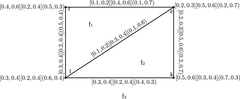
FIGURE 3. Strength of the faces.

4 Cubic intuitionistic dual graph

In this section, the notion of a cubic intuitionistic dual graph (CIDG) is presented. We can draw a CIDG only if the graph is either planar or have planarity measure ${\mathfrak{f}}_N\le ⟨[0.33,0.33],0.33⟩$ and ${\mathfrak{f}}_M\ge ⟨[0.67,0.67],0.67⟩$. The edges of the CIPG correspond to the edges of the CIDG, while faces of the CIPG correspond to the vertices of the CIDG.

Definition 4.1. Let $\mathbb{G}=(\mathbb{V},\mathbb{B})$ be a CIPG such that $\mathbb{B}=\{(f,t),⟨[{\mathfrak{H}}_v^{-},{\mathfrak{H}}_v^{+}],[{\mathfrak{L}}_v^{-},{\mathfrak{L}}_v^{+}],({\mathfrak{H}}_v^{*},{\mathfrak{L}}_v^{*})⟩,v=\mathrm{1,2},\dots ,k:ft\in \mathfrak{S}\times \mathfrak{S})$ and ${\mathfrak{f}}_1,{\mathfrak{f}}_2,\dots ,{\mathfrak{f}}_n$ be the faces of $\mathbb{G}$ surrounded by edges. So, ${\mathbb{G}}^{\prime }=({\mathbb{I}}^{\prime },{\mathbb{S}}^{\prime })$ is the dual graph of the CIPG, where the vertex set is denoted by ${\mathbb{I}}^{\prime }$ and the edge set is denoted by ${\mathbb{S}}^{\prime }$. The following expression is used to calculate the membership and non-membership values of vertices:

$\mathfrak{J}\left(y_v\right)=\left\{\mathit{max}{\mathfrak{H}}_v\left(f,t\right),v=\mathrm{1,2},\dots ,k:ft\text{is one of the edge}\text{along the cubic intuitionistic faces}\right\},$

$\mathfrak{A}\left(y_v\right)=\left\{\mathit{min}{\mathfrak{L}}_v\left(f,t\right),v=\mathrm{1,2},\dots ,k:ft\text{\hspace{0.17em}is\hspace{0.17em}\hspace{0.17em}one\hspace{0.17em}\hspace{0.17em}of\hspace{0.17em}\hspace{0.17em}the\hspace{0.17em}\hspace{0.17em}edge}\text{along\hspace{0.17em}\hspace{0.17em}the\hspace{0.17em}\hspace{0.17em}cubic\hspace{0.17em}\hspace{0.17em}intuitionistic\hspace{0.17em}\hspace{0.17em}faces}\right\}.$

It is noted that two faces may share more than one common edge. As a result, vertices of the CIDG may have several edges crossing them. If ${\mathfrak{L}}^v(z_i,z_j)$ and ${\mathfrak{A}}^v(z_i,z_j)$ indicate the non-membership and membership values, respectively, of an edge (z_i, z_j), then for the membership and non-membership values of the cubic intuitionistic edge of the CIDG, we have

$\mathfrak{L}{\left(z_i,z_j\right)}_v={\mathfrak{L}}^v{\left(f,t\right)}_{p}and\mathfrak{A}{\left(z_i,z_j\right)}_v={\mathfrak{A}}^v{\left(f,t\right)}_p,$

where v = 1, 2, … , k and k is the number of common edges. The pendant vertex in the CIPG is associated with a loop in the CIDG with the degrees of membership and non-membership being the same as that of the pendant vertex. According to the value of planarity [18][0, 0](1, 0), the graph CIDG is always planar. By taking the vertices of the CIDG as the faces and the edges as the edges of the CIPG, we may create the CIPG from the CIDG.

Example 4.2. Let ${\mathbb{G}}^{*}=(\mathfrak{S},\mathbb{E})$ be a crisp graph of the CIPG $\mathbb{G}=(\mathbb{V},\mathbb{B})$. Tables 2, 3 show the values of vertices and edges, respectively.The degrees of three faces, as shown in Figure 4, are calculated. It is noted that in the CIDG, the vertices {k₁, k₂, k₃} are the faces of the graph. The membership and non-membership values of vertices of CIDG or faces are calculated as follows:

$\mathfrak{J}\left(k_1\right)=\langle \left[\max \left\{0.2,0.3,0.2\right\}\right],\max \left\{0.1,0.2,0.1\right\},\max \left\{0.2,0.1,0.1\right\}\rangle =\langle \left[0.2,0.3\right],0.2\rangle ,$

$\mathfrak{A}\left(k_1\right)=\langle \left[\min \left\{0.3,0.5,0.5\right\}\right],\min \left\{0.2,0.4,0.4\right\},\min \left\{0.7,0.7,0.7\right\}\rangle =\langle \left[0.4,0.5\right],0.7\rangle ,$

$\mathfrak{J}\left(k_2\right)=\langle \left[\max \left\{0.2,0.2,0.2\right\}\right],\max \left\{0.1,0.1,0.1\right\},\max \left\{0.7,0.1,0.1\right\}\rangle =\langle \left[0.1,0.2\right],0.7\rangle ,$

$\mathfrak{A}\left(k_2\right)=\langle \left[\min \left\{0.6,0.6,0.5\right\}\right],\min \left\{0.4,0.4,0.4\right\},\min \left\{0.3,0.7,0.7\right\}\rangle =\langle \left[0.4,0.5\right],0.3\rangle ,$

$\mathfrak{J}\left(k_3\right)=\langle \left[\max \left\{0.3,0.2,0.2,0.2\right\}\right],\max \left\{0.2,0.1,0.1,0.1\right\},\max \left\{0.1,0.1,0.7,0.1\right\}\rangle =\langle \left[0.2,0.3\right],0.7\rangle ,$

$\mathfrak{A}\left(k_3\right)=\langle \left[\min \left\{0.4,0.4,0.4,0.2\right\},\min \left\{0.5,0.6,0.6,0.3\right\}\right],\min \left\{0.7,0.7,0.3,0.7\right\}\rangle =\langle \left[0.2,0.3\right],0.3\rangle .$

The membership and non-membership values of the new edges are calculated as:$\mathfrak{H}(k_1,k_2)=\mathfrak{H}(s,r)=⟨[0.1,0.2][0.4,0.5](0.1,0.7)⟩$; there are two common edges between the vertices (k₁, k₃) and (k₂, k₃), so $\mathfrak{H}(k_1,k_3)=\mathfrak{H}(l,s)=⟨[0.1,0.2][0.2,0.3](0.2,0.7)⟩$, $\mathfrak{H}(k_1,k_3)=\mathfrak{H}(l,r)=⟨[0.2,0.3][0.4,0.5](0.1,0.7)⟩$, $\mathfrak{H}(k_2,k_3)=\mathfrak{H}(e,r)=⟨[0.1,0.2][0.4,0.5](0.1,0.7)⟩$, and $\mathfrak{H}(k_2,k_3)=\mathfrak{H}(s,e)=⟨[0.1,0.2][0.4,0.6](0.7,0.3)⟩$. Hence, the required edge set of the CIDG is

$\begin{array}{ccc}\hfill {\mathbb{I}}^{\prime }& =\hfill & \left\{\left(k_1{k}_2,\left[0.1,0.2\right]\left[0.4,0.5\right]\left(0.1,0.7\right)\right),\left(k_1{k}_3,\left[0.1,0.2\right]\left[0.2,0.3\right]\left(0.2,0.7\right)\right),\left(k_1{k}_3,\left[0.2,0.3\right]\left[0.4,0.5\right]\left(0.1,0.7\right)\right),\right.\hfill \\ \hfill & \hfill & \left.\left(k_2{k}_3,\left[0.1,0.2\right]\left[0.4,0.5\right]\left(0.1,0.7\right)\right),\left(k_2{k}_3,\left[0.1,0.2\right]\left[0.4,0.6\right]\left(0.7,0.3\right)\right)\right\}.\hfill \end{array}$

TABLE 2

TABLE 2. Value of the vertices.

TABLE 3

TABLE 3. Value of the edges.

FIGURE 4

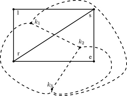
FIGURE 4. Example of the CIDG.

Theorem 4.3. We consider a CIPG $\mathbb{G}$ having the number of vertices, edges, and faces of $\mathbb{G}$ as $\mathbb{V}$, $\mathbb{E}$, and $\mathbb{F}$, respectively. Take the dual graph ${\mathbb{G}}^{\prime }$ of $\mathbb{G}$ with the number of vertices, edges, and faces as ${\mathbb{V}}^{\prime }$, ${\mathbb{E}}^{\prime }$, and ${\mathbb{F}}^{\prime }$, respectively, then

1. ${\mathbb{E}}^{\prime }=\mathbb{E}$,

2. ${\mathbb{F}}^{\prime }=\mathbb{F}$,

3. ${\mathbb{V}}^{\prime }=\mathbb{V}$.

5 Application to the airline system

In the past, individuals had to take a ship or a land vehicle, which was exhausting and time-consuming. The likelihood of becoming lost or getting into an accident increases as a result. The emergence of the airline system, a quick mode of transportation that is especially helpful when on a strict timetable, has all but eliminated this issue. Airline routes occasionally cross paths (intersection) which can either be eliminated or not depending on the degree of planarity.

The airline route system is represented in Figure 5. The vertices of this diagram denote the countries, and its edges stand in for the air routes that link them. Here, the vertices have values ⟨[0.5, 0.5][0.5, 0.5](0.5, 0.5)⟩, or in other words, have half degrees of membership and non-membership. Now, we select the level of membership and non-membership for edges, which depends on a range of variables including the ticket prices, the frequency of flights, festivals, and more. There may be more flights on that route and more passengers traveling by the plane if the ticket price is affordable, increasing the likelihood of an encounter. There will be more travel as a result. The major issue, which is the crowd of people or the number of flights, is connected to all of these elements in some manner. As a result, chosen from the closed interval [0,1], the degree of membership and non-membership among edges will be vague or unclear.

FIGURE 5

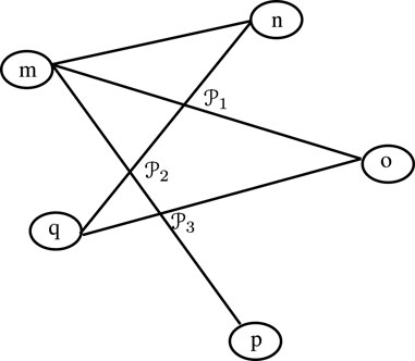
FIGURE 5. Network of an airline.

A CIPG is connected to both a continuous and a particular operation. Although a fuzzy interval denotes a continuous process, a fuzzy number denotes a discrete process. So using the present as a number and the future as an interval, we examine the path’s intersection at both the current and future dates. There is a possibility that there is a crossover that is currently unavailable will be required some other day; similarly, there would be a situation that a currently blocked intersection due to a festival or other circumstance may be needed in future. Table 4 demonstrates the edge membership and non-membership degree.Because the intersection might increase with the number of aircraft every day, there is a direct correlation between the crowd and the intersection. We utilize the approach in Table 5 to determine the degree of planarity.From Figure 5, it is evident that ${\mathfrak{p}}_1,{\mathfrak{p}}_2$ and ${\mathfrak{p}}_3$ are points of intersection due to the edges (fk, gl), (fk, lh), and (kg, lh). The strength of edges is computed as follows:

$M_{qn}=\langle \left[\frac{{\mathfrak{H}}_{qn}^{-}}{\min \left({\mathfrak{J}}_q^{+},{\mathfrak{J}}_q^{+}\right)},\frac{{\mathfrak{H}}_{qn}^{+}}{\min \left({\mathfrak{J}}_q^{+},{\mathfrak{J}}_q^{+}\right)}\right],\frac{{\mathfrak{H}}_{qn}^{*}}{\min \left({\mathfrak{J}}_q^{*},{\mathfrak{J}}_q^{*}\right)}\rangle =\langle \left[\frac{0.3}{0.5},\frac{0.4}{0.5}\right],\frac{0.1}{0.5}\rangle =\left(\left[0.6,0.8\right],0.2\right),$

$N_{qn}=\langle \left[\frac{{\mathfrak{L}}_{qn}^{-}}{\max \left({\mathfrak{A}}_q^{+},{\mathfrak{A}}_q^{+}\right)},\frac{{\mathfrak{L}}_{qn}^{+}}{\max \left({\mathfrak{A}}_q^{+},{\mathfrak{A}}_q^{+}\right)}\right],\frac{{\mathfrak{L}}_{qn}^{*}}{\max \left({\mathfrak{A}}_q^{*},{\mathfrak{A}}_q^{*}\right)}\rangle =\langle \left[\frac{0.4}{0.5},\frac{0.5}{0.5}\right],\frac{0.5}{0.5}\rangle =\left(\left[0.8,1\right],1\right).$

So I_qn = ⟨[0.6, 0.8], [0.8, 1](0.2, 1)⟩.

TABLE 4

TABLE 4. Membership and non-membership values of edges.

TABLE 5

TABLE 5. Algorithm to determine intersecting routes.

Similarly, the strength of the other edges is determined as follows:

$\begin{array}{ccc}\hfill I_{mo}& =\hfill & ⟨\left[0.6,1\right]\left[0.6,0.8\right]\left(\mathrm{1,0.6}\right)⟩,\hfill \\ \hfill I_{qo}& =\hfill & ⟨\left[0.4,1\right]\left[0.2,0.4\right]\left(0.8,0.4\right)⟩,\hfill \\ \hfill I_{mp}& =\hfill & ⟨\left[0.6,0.8\right]\left[0.2,0.8\right]\left(\mathrm{1,0.2}\right)⟩.\hfill \end{array}$

Thus, ${\mathcal{P}}_1$ is computed as

$M_{{\mathcal{P}}_1}=\left(\left[\frac{M_{qn}^{-}+M_{mo}^{-}}{2},\frac{M_{qn}^{+}+M_{mo}^{+}}{2}\right],\frac{M_{qn}^{*}+M_{mo}^{*}}{2}\right)=\left(\left[\frac{0.6+0.6}{2},\frac{0.8+1}{2}\right],\frac{0.2+1}{2}\right)=\left(\left[0.6,0.9\right],0.6\right),$

$N_{{\mathcal{P}}_1}=\left(\left[\frac{N_{qn}^{-}+M_{mo}^{-}}{2},\frac{N_{qn}^{+}+M_{mo}^{+}}{2}\right],\frac{N_{qn}^{*}+N_{mo}^{*}}{2}\right)=\left(\left[\frac{0.6+0.6}{2},\frac{1+0.8}{2}\right],\frac{1+0.6}{2}\right)=\left(\left[0.6,0.9\right],0.8\right).$

So the cutting value at ${\mathcal{P}}_1$ is

$I_{{\mathcal{P}}_1}=⟨\left[0.6,0.9\right],\left[0.6,0.9\right],\left(0.6,0.8\right)⟩.$

Similarly, ${\mathcal{P}}_2$ and ${\mathcal{P}}_3$ are calculated by repeating the process.

$I_{{\mathcal{P}}_2}=⟨\left[0.6,0.8\right],\left[0.5,0.45\right],\left(0.6,0.6\right)⟩,$

$I_{{\mathcal{P}}_3}=⟨\left[0.5,0.9\right],\left[0.2,0.6\right],\left(0.9,0.3\right)⟩.$

The membership and non-membership degrees are finally determined as

${\mathfrak{F}}_M=\langle \left[\frac{1}{1+0.9+0.8+0.9},\frac{1}{1+0.6+0.6+0.5}\right],\frac{1}{1+0.6+0.6+0.9}\rangle =\langle \left[0.27,0.37\right],0.32\rangle ,$

${\mathfrak{F}}_N=\langle \left[\frac{1}{1+0.9+0.45+0.6},\frac{1}{1+0.6+0.5+0.2}\right],\frac{1}{1+0.8+0.6+0.3}\rangle =\langle \left[0.33,0.43\right],0.37\rangle .$

Clearly, the planarity value is $\mathfrak{F}=⟨[0.27,0.37],[0.33,0.43],(0.32,0.37)⟩$. We can see ${\mathfrak{F}}_M\le ([0.67,0.67],0.67)$ and ${\mathfrak{F}}_N\ge ([0.33,0.33],0.33)$, which demonstrates that intersections between airline routes are essential and cannot be avoided. Here, we observe that the airline route is currently congested, and it is imperative to promptly clear the airline route before the arrival of the next plane, or else we might face a potential collapse. Therefore, it is recommended that either the airline adjusts its time schedule, or alternatively, the plane may need to remain in the air if the route is not available. It is also noted that the intersection of two routes is irrelevant if ${\mathfrak{F}}_M\ge ([0.67,0.67],0.67)$ and ${\mathfrak{F}}_N\le ([0.33,0.33],0.33)$. Thus, the intersection of airline routes will be required at both times (in the future and also at present time).

6 Comparison with already existing methods

There are already existing methods, such as the intuitionistic fuzzy planar graph and interval-valued intuitionistic planar graph, which can be used to determine if a discrete process is planar or if an interval representing a continuous process is planar, respectively. However, CIPGs combine the strengths of both these methods. An intuitionistic graph may be planar, but interval-valued intuitionistic graphs may not always be so. To avoid redundant discussions, we use both of them in this research article to thoroughly inspect planarity.

In cubic planar graphs, interval-valued planar graphs and fuzzy planar graphs are considered simultaneously [45]. However, we use a more sophisticated technique that involves the use of two intervals and two fuzzy numbers, where one interval indicates the membership value and the other indicates the non-membership value, and similarly for the fuzzy numbers.

7 Conclusion

Graph theory is applied in system analysis, transportation difficulties, and a variety of other fields including computer science (algorithms and computations) and electrical engineering (communication networks and coding theory) . However, because some features of graph theory problems are ambiguous and unclear, we can answer them utilizing fuzzy graph theory. We introduced the concept of CIPGs, which are a hybrid of interval-valued intuitionistic planar graphs and intuitionistic fuzzy planar graphs. We proposed the terms CIMS and CIMG. We gained knowledge about how to determine the edge strength. We also talk about CIPG’s planarity. Using a cubic intuitionistic cubic valued number, we were able to construct the formula for the degree of planarity. We also showed how, if the degree of planarity is more than or equal to 0.67, the CIPG can be transformed into the CIDG. We also discovered the CIDG faces’ strength. There are several graph networks in which crossing between edges causes a difficulty and avoiding this overlap can be challenging at times. We can deal with such problems using a planar graph. Planar graphs can be used to build circuits and road networks. We gave an example of the airline system to check crossing between edges by finding the planarity value. After determining the values, we have concluded that either the airline adjusts its time schedule, or alternatively, the plane may need to remain in the air if the route is not available.

A limitation to our technique lies in its applicability solely to undirected graphs. A cubic Pythagorean fuzzy planar network is our future direction.

Data availability statement

The original contributions presented in the study are included in the article/Supplementary Material; further inquiries can be directed to the corresponding author.

Author contributions

GF: conceptualization, funding acquisition, methodology, and writing–review and editing. UA: conceptualization, formal analysis, investigation, methodology, supervision, and writing–review and editing. AR: conceptualization, formal analysis, investigation, writing–original draft, and writing–review and editing. AK: formal analysis, investigation, methodology, and writing–original draft. JS: conceptualization, formal analysis, methodology, and writing–review and editing.

Funding

This work was supported by the National Natural Science Foundation of China with grant number 61972107.

Conflict of interest

The authors declare that the research was conducted in the absence of any commercial or financial relationships that could be construed as a potential conflict of interest.

Publisher’s note

All claims expressed in this article are solely those of the authors and do not necessarily represent those of their affiliated organizations, or those of the publisher, the editors, and the reviewers. Any product that may be evaluated in this article, or claim that may be made by its manufacturer, is not guaranteed or endorsed by the publisher.

References

1. Amer A, Irfan M, Rehman HU. Computational aspects of line graph of boron triangular nanotubes. United Kingdom: Mathematical Methods in the Applied Sciences (2021).

Google Scholar

2. Amer A, Naeem M, Rehman HU, Irfan M, Saleem MS, Yang H. Edge version of topological degree based indices of Boron triangular nanotubes. J Inf Optimization Sci (2020) 41(4):973–90. doi:10.1080/02522667.2020.1743505

CrossRef Full Text | Google Scholar

3. Irfan M, Rehman HU, Almusawa H, Rasheed S, Baloch IA. M-polynomials and topological indices for line graphs of chain silicate network and h-naphtalenic nanotubes. J Math (2021) 2021:1–11. doi:10.1155/2021/5551825

CrossRef Full Text | Google Scholar

4. Yasmeen F, Ali K, Shahid M. Entropy Measures Some Nanotubes Polycyclic Aromatic Comp (2022) 42(9):6592–604.

CrossRef Full Text

5. Zadeh LA. Fuzzy sets. Inf Control (1965) 8:338–53. doi:10.1016/s0019-9958(65)90241-x

CrossRef Full Text | Google Scholar

6. Rosenfeld A. Fuzzy graphs. In: Fuzzy sets and their applications to cognitive and decision processes. Cambridge: Academic Press (1975). p. 77–95.

CrossRef Full Text | Google Scholar

7. Kaufmann A. Introduction to the theory of fuzzy sets. In: Fundamental theoretical elements. New York: Academic Press (1980).

Google Scholar

8. Mordeson JN, Nair PS. Fuzzy graphs and fuzzy hypergraphs. In: Physica (2012). doi:10.1007/978-3-7908-1854-3

CrossRef Full Text | Google Scholar

9. Shannon A, Atanassov K. A first step to a theory of the intuitionistic fuzzy graphs. In: D akov, editor. Proc. Of the first workshop on fuzzy based expert systems (1994). p. 59–61.

Google Scholar

10. Parvathi R, Karunambigai MG, Atanassov KT (2009). Operations on intuitionistic fuzzy graphs. Proceedings of the 2009 IEEE international conference on fuzzy systems. August 2009 Korea p. 1396–401.

CrossRef Full Text | Google Scholar

11. Akram M, Alshehri NO. Intuitionistic fuzzy cycles and intuitionistic fuzzy trees. Scientific World J (2014) 2014:1–11. Article ID 305836. doi:10.1155/2014/305836

PubMed Abstract | CrossRef Full Text | Google Scholar

12. Jabbar A, Naoom JH, Ouda EH. Fuzzy dual graph. Al-Nahrain J Sci (2009) 12(4):168–171.

Google Scholar

13. Samanta S, Pal M. Fuzzy planar graphs. IEEE Trans fuzzy Syst (2015) 23(6):1936–42. doi:10.1109/TFUZZ.2014.2387875

CrossRef Full Text | Google Scholar

14. Alshehri N, Akram M. Intuitionistic fuzzy planar graphs. Discrete Dyn Nat Soc (2014) 2014:1–9. doi:10.1155/2014/397823

CrossRef Full Text | Google Scholar

15. Akram M, Mohsan Dar J, Farooq A. Planar graphs under Pythagorean fuzzy environment. Mathematics (2018) 6(12):278. doi:10.3390/math6120278

CrossRef Full Text | Google Scholar

16. Nirmala G, Dhanabal MK. Special planar fuzzy graph configurations. Internatinal J Scientific Reserch Publ (2012) 2(7):2250–3153.

Google Scholar

17. Pal A, Samanta S, Pal M (2013). Concept of fuzzy planar graphs. Proceedings of the 2013 Science and Information Conference. October 2013, London p. 557–63.

Google Scholar

18. Ahmad U, Nawaz I. Directed rough fuzzy graph with application to trade networking. Comput Appl Math (2022) 41(8):366. doi:10.1007/s40314-022-02073-0

CrossRef Full Text | Google Scholar

19. Ahmad U, Batool T. Domination in rough fuzzy digraphs with application. Soft Comput (2023) 27(5):2425–42. doi:10.1007/s00500-022-07795-1

CrossRef Full Text | Google Scholar

20. Ahmad U, Khan NK, Saeid AB. Fuzzy topological indices with application to cybercrime problem. Granular Comput (2023) 1-14:967–80. doi:10.1007/s41066-023-00365-2

CrossRef Full Text | Google Scholar

21. Ahmad U, Nawaz I. Wiener index of a directed rough fuzzy graph and application to human trafficking. J Intell Fuzzy Syst (2023) 44:1479–95. doi:10.3233/jifs-221627

CrossRef Full Text | Google Scholar

22. Ahmad U, Sabir M. Multicriteria decision-making based on the degree and distance-based indices of fuzzy graphs. Granular Comput (2022) 8:793–807. doi:10.1007/s41066-022-00354-x

CrossRef Full Text | Google Scholar

23. Akram M, Ahmad U, Rukhsar S, Karaaslan F. Complex Pythagorean fuzzy threshold graphs with application in petroleum replenishment. J Appl Math Comput (2022) 68(2022):2125–50. doi:10.1007/s12190-021-01604-y

CrossRef Full Text | Google Scholar

24. Kosari S, Shao Z, Rao Y, Liu X, Cai R, Rashmanlou H. Some types of domination in vague graphs with application in medicine. J Multi-valued Logic Soft Computing (2023) 40:203–19.

Google Scholar

25. Rao Y, Kosari S, Shao Z, Talebi AA, Mahdavi A, Rashmanlou H. New concepts of intuitionistic fuzzy trees with applications. Int J Comput Intell Syst (2021) 14:175–12. doi:10.1007/s44196-021-00028-7

CrossRef Full Text | Google Scholar

26. Rashmanlou H, Borzooei RA. Vague graphs with application. J Intell Fuzzy Syst (2016) 30(6):3291–9. doi:10.3233/ifs-152077

CrossRef Full Text | Google Scholar

27. Rashmanlou H, Jun YB, Borzooei RA. More results on highly irregular bipolar fuzzy graphs. Ann Fuzzy Math Inform (2014) 8(1):149–68.

Google Scholar

28. Samanta S, Pal M, Rashmanlou H, Borzooei RA. Vague graphs and strengths. J Intell Fuzzy Syst (2016) 30(6):3675–80. doi:10.3233/ifs-162113

CrossRef Full Text | Google Scholar

29. Samanta S, Dubey VK, Sarkar B. Measure of influences in social networks. Appl Soft Comput (2021) 99(2021):106858. doi:10.1016/j.asoc.2020.106858

CrossRef Full Text | Google Scholar

30. Samanta S, Sarkar B. A study on generalized fuzzy graphs. J Intell Fuzzy Syst (2018) 35(3):3405–12. doi:10.3233/jifs-17285

CrossRef Full Text | Google Scholar

31. Shoaib M, Kosari S, Rashmanlou H, Malik MA, Rao Y, Talebi Y, et al. Notion of complex pythagorean fuzzy graph with properties and application. J Mult.-Valued Log Soft Comput (2020) 34(5-6):553–86.

Google Scholar

32. Shao Z, Kosari S, Rashmanlou H, Shoaib M. New concepts in intuitionistic fuzzy graph with application in water supplier systems. Mathematics (2020) 8(8):1241. doi:10.3390/math8081241

CrossRef Full Text | Google Scholar

33. Shi X, Kosari S, Talebi AA, Sadati SH, Rashmanlou H. Investigation of the main energies of picture fuzzy graph and its applications. Int J Comput Intell Syst (2022) 15(1):31. doi:10.1007/s44196-022-00086-5

CrossRef Full Text | Google Scholar

34. Shi X, Kosari S. Certain properties of domination in product vague graphs with novel application in medicine. Front Phys (2021) 9:385.

CrossRef Full Text | Google Scholar

35. Zeng S, Shoaib M, Ali S, Smarandache F, Rashmanlou H, Mofidnakhaei F. Certain Properties of Single-valued neutrosophic graph with application in food and agriculture organization. Int J Comput Intell Syst (2021) 14(1):1516–40. doi:10.2991/ijcis.d.210413.001

CrossRef Full Text | Google Scholar

36. Zadeh LA. The concept of a linguistic variable and its application to approximate reasoning—I. Inf Sci (1975) 8(3):199–249. doi:10.1016/0020-0255(75)90036-5

CrossRef Full Text | Google Scholar

37. Akram M, Dudek WA. Interval-valued fuzzy graphs. Comput Math Appl (2011) 61(2):289–99. doi:10.1016/j.camwa.2010.11.004

CrossRef Full Text | Google Scholar

38. Akram M, Yousaf MM, Dudek WA. Self centered interval-valued fuzzy graphs. Afrika Matematika (2015) 26(5):887–98. doi:10.1007/s13370-014-0256-9

CrossRef Full Text | Google Scholar

39. Qiang X, Kosari S, Chen X, Talebi AA, Muhiuddin G, Sadati SH. A novel description of some concepts in interval-valued intuitionistic fuzzy graph with an application. Adv Math Phys (2022) 2022:1–15. ID 2412012. doi:10.1155/2022/2412012

CrossRef Full Text | Google Scholar

40. Talebi AA, Rashmanlou H, Sadati SH. Interval-valued intuitionistic fuzzy competition graph. J Multiple-Valued Logic Soft Comput (2020) 34.

Google Scholar

41. Pramanik T, Samanta S, Pal M. Interval-valued fuzzy planar graphs. Int J machine Learn cybernetics (2016) 7(4):653–64. doi:10.1007/s13042-014-0284-7

CrossRef Full Text | Google Scholar

42. Jun YB, Kim CS, Yang KO. Cubic sets. Ann Fuzzy Math Inform (2012) 4(1):83–98.

Google Scholar

43. Rashid S, Yaqoob N, Akram M, Gulistan M. Cubic graphs with application. Int J Anal Appl (2018) 16(5):733–50.

Google Scholar

44. Khan SU, Jan N, Ullah K, Abdullah L. Graphical structures of cubic intuitionistic fuzzy Information. J Math (2021) 2021:1–21. Article ID 9994977. doi:10.1155/2021/9994977

CrossRef Full Text | Google Scholar

45. Muhiuddin G, Hameed S, Rasheed A, Ahmad U. Cubic planar graph and its application to road network. Math Probl Eng (2022) 2022:1–12. doi:10.1155/2022/5251627

CrossRef Full Text | Google Scholar

46. Muhiuddin G, Hameed S, Ahmad U. Cubic pythagorean fuzzy graphs. J Math (2022) 2022:1–25. Article ID 1144666. doi:10.1155/2022/1144666

CrossRef Full Text | Google Scholar

47. Li L, Kosari S, Sadati SH, Talebi AA. Concepts of vertex regularity in cubic fuzzy graph structures with an application. Front Phys (2023) 10. doi:10.3389/fphy.2022.1087225

CrossRef Full Text | Google Scholar

48. Yager RR. On the theory of bags. Int J Gen Syst (1986) 13(1):23–37. doi:10.1080/03081078608934952

CrossRef Full Text | Google Scholar

49. Shinoj TK, John SJ. Intuitionistic fuzzy multisets and its application in medical diagnosis. World Acad Sci Eng Tech (2012) 6(1):1418–21.

Google Scholar

50. Atanassov KT. Intuitionistic fuzzy sets. Fuzzy sets Syst (1986) 20:87–96. doi:10.1016/s0165-0114(86)80034-3

CrossRef Full Text | Google Scholar

51. Atanassov KT. More on intuitionistic fuzzy sets. Fuzzy sets Syst (1989) 33(1):37–45. doi:10.1016/0165-0114(89)90215-7

CrossRef Full Text | Google Scholar