 Gonzalo G. Rodriguez
 Clemar A. Schürrer2
 Esteban Anoardo
94% of researchers rate our articles as excellent or good
Learn more about the work of our research integrity team to safeguard the quality of each article we publish.
Find out more
ORIGINAL RESEARCH article
Front. Phys., 02 November 2023
Sec. Medical Physics and Imaging
Volume 11 - 2023 | https://doi.org/10.3389/fphy.2023.1249771
This article is part of the Research TopicAdvances and Applications in Portable Magnetic Resonance Imaging (MRI)View all articles
Understanding the effects of the magnetic field time instabilities in magnetic resonance imaging (MRI) is fundamental for the success of portable and low-cost MRI hardware based on electromagnets. In this work we propose a magnetic field model that considers the field instability in addition to the inhomogeneity. We have successfully validated the model on signals acquired with a commercial NMR instrument. It was used to simulate the image defects due to different types of instability for both the spin-echo and the gradient-echo sequences. We have considered both random field fluctuations, and an instability having a dominant harmonic component. Strategies are suggested to minimize the artifacts generated by these instabilities. Images were acquired using a home-made MRI relaxometer to show the consistency of the analysis.
The development of low field MRI instruments (<0.2 T) is growing drastically [1–3] motivated by the possibility of cost reductions [4, 5], portability [6–10], and contrast-enhancement [11]. However, critical points to consider are the lower signal to noise ratio (SNR) [12], magnetic field homogeneity [9], and magnetic field stability [13]. These limitations may strongly affect the image quality by introducing biasing and artifacts. Therefore, the success of low field scanners strongly depends on our ability to minimize or compensate these undesired effects.
In MRI experiments the SNR degrades with the magnetic flux density (B0) as B0x, with an exponent x ranging from 1.65 to 1.75 [12, 14]. In consequence, the SNR working conditions for low-field MRI can be much poorer that those usually available at high-field MRI. However, the SNR can be improved by different means, from a simple signal averaging to different hardware and computational contraptions. Some explored hardware solutions include, among other, hyperpolarization schemes [11], magnetic field-cycling technology [3, 13, 15], single or multiple receiver channels using superconducting quantum interference devices (SQUID) [16–18] and coupling to external resonators or magnetic lenses for signal enhancement [19–21]. Specially designed pulse sequences are also considered [22, 23], while image pos-processing can be used to artificially enhance the image SNR [24, 25].
Against the natural lower SNR of the acquired signal at low magnetic field conditions, some advantages of the methodology are compensating this fact. Spin-lattice (T1) relaxation times are usually much shorter at low magnetic fields [26], thus allowing a higher number of scans (signal acquisitions) per unit of time. The specific absorption rate (SAR) is proportional to the square of the magnetic field. Consequently, at low magnetic fields, pulse sequences with high flip angles or increased duty-cycles are favored. In addition, the effects of superparamagnetic nanoparticles in modulating the spin relaxation are very relevant at low magnetic fields [27], thus allowing an efficient contrast enhancement [7, 28]. It is opportune to mention that the SNR of the image is related to the contrast-to-noise ratio (CNR), which can be increased by a proper use of contrast agents [29] and/or mathematically manipulated through computational post processing of the acquired image [30, 31].
Compact magnet designs and imperfect mechanical assembling are usually associated with highly inhomogeneous magnetic fields, with inhomogeneities orders of magnitude bigger than superconducting magnets [8, 13]. Notwithstanding this feature, it has been shown that MRI images with reasonable quality are achievable under high inhomogeneities [32, 33], including inhomogeneities higher than 1,000 ppm [34, 35]. Image distortions due to magnetic field inhomogeneities can be compensated by different methods [36–38].
The use of non-cryogenic magnets usually implies dealing with magnetic field instability. This feature is usually an important point to consider if electromagnets are chosen. However, the implementation of electromagnets in MRI prototypes has shown promising results [2, 3, 39, 40]. This approach is attractive since it allows switching the magnetic field [41, 42], then enabling the acquisition of images with contrasts unavailable at fixed magnetic fields [43, 44]. Recent examples are the combination of field cycling MRI with superparamagnetic nanoparticles [45] and proton double irradiation [46].
Despite the high potential associated with the use of electromagnets in low-field MRI, the study of magnetic field instability-induced artifacts is a topic that has hardly been considered in the literature. In the context of MRI, this point is usually skipped although some mentions can be found in hardware-related papers [47, 48]. In addition, the main strategies for artifact correction due to low field stability are post-processing methods [37, 49], and most of them were focused on mitigating motion artifacts at high magnetic fields [50, 51]. Therefore, the practically nonexistent studies on this area represent a limitation for the development of the new generation of low field MRI scanners based on electromagnets.
In reference 37 we proposed an algorithm to correct instabilities and inhomogeneities for Cartesian spin-echo acquisitions. The method consists in a two step sequential algorithm considering both random field fluctuations and field inhomogeneity corrections, neglecting any potential correlation between them. In this work we made an exhaustive analysis of the role of magnetic field stability in the context of MRI. We discuss the relationship between magnetic field stability and homogeneity in the context of both the NMR and MRI signal. The presented model allows observing that spin dephasing due to magnetic field instability is proportional to the field strength at which the imaging sequence is applied. This fact represents a key feature supporting the use of electromagnets in low-field MRI technology.
We present a simple mathematical model for an inhomogeneous and unstable magnetic field, and performed simulations using this model for the spin-echo and the gradient-echo pulse sequences [52]. For the simulations, we considered two types of instabilities, one completely random and the case where a dominant monochromatic harmonic component is present. NMR experiments were done to test and validate our model and simulations. Experimental images were acquired in a resistive homemade MRI relaxometer with different echo times, in order to characterize the image degradation due to instability. Finally, strategies are discussed to minimize the undesirable effects induced by magnetic field instability. This work is important in view of a potential reduction of costs associated to the involved hardware.
In this section we consider a magnetic field model for an electromagnet (switched or not) that is fed by a current source. In this frame, we consider a realistic picture in which the magnet homogeneity and the current stability are not perfect. However, we will neglect a potential time dependence of the magnetic field homogeneity.
The magnetic flux density at a given position r (x,y,z), B (r,t), can be factorized as a product of two well defined independent functions. The first one, C(r) is associated with the spatial dependence of the generated magnetic field, which essentially depends on the magnet geometry. This functional also includes magnet machining and assembly imperfections that degrade the generated field homogeneity. The second function I(t) is the current in the circuit. If we define the mean temporal value I0 of the current then, I(t) = I0+ΔI(t). ΔI(t) is associated with the temporal instability of the current, which is mainly attributed to the quality and performance of the control and power electronics of the magnet current power supply. In the same way, C(r) can be expressed as the sum of a constant C0 = C (0) (where the position 0 = (0,0,0) is located at the geometric center of the magnet), plus a position-dependent term ΔC(r). The proposed factorization allows us to clearly separate the spatial inhomogeneities from the temporal instability (described by ΔC(r) and ΔI(t) respectively) in the factors that describe the evolution of the phase during the image acquisition (see Eq. (4)). Through these considerations, it is possible to express the magnetic field as it is shown in Eq. (1):
Applying the distributive property of the product, B (r,t) can be expressed as:
The first term of Eq. 2 can be associated with the main magnetic field value B0. The second term can be interpreted as the magnetic field inhomogeneity while the third term as the magnetic field instability. The last term is typically much smaller than the others and it will be neglected. Therefore, neglecting the last term, the magnetic field can be approximated as:
The fact that C and I have been considered as independent variables is an approximation. The model does not consider variations in the geometry of the magnet during the experiment. This condition is fulfilled in most cases, although it can be violated in extreme situations. Nevertheless, this formalization is adequate to describe and interpret the effects of magnetic field instability in several NMR and MRI experiments.
As the free induction decay (FID) is the simplest experiment in NMR, it is an appropriate test for our magnetic field model. Furthermore, if the model is accurate, it can be useful to understand the relationship between the magnetic field inhomogeneity and stability in complex experiments.
The signal is modeled without considering relaxation effects as the magnetic field inhomogeneity and instability are considered to be dominant. That means that the signal loss attributed to T1 and T2 is much smaller than the loss induced by the magnetic field deviations. The defacing during the RF pulses is neglected. This is equivalent to assuming that the RF pulses are perfect and infinitely short. Defining ρ(r) as the spin density of the sample and γ the proton gyromagnetic ratio, the FID signal can be modeled as:
In Eq. (4), we integrate over the whole space (the integrals limits go from -∞ to ∞), and the dimensions of the sample are contained in
According to this scheme, if the following condition is satisfied:
then the NMR signal will show a certain immunity to the magnetic field instability. This means that the effects of the instability on the NMR signal will be less relevant if the inhomogeneity is dominant over the instability. In other words, as the frequency spectrum of the instability is constrained within the bandwidth covered by the field inhomogeneity, the NMR signal gains immunity against magnetic field fluctuations (periodic and random noise). This fact constitutes a key-feature for gaining signal stability against magnetic field or current instability through controlled homogeneity degradation. In section 2.3.1 we will present experimental evidence that verify this theoretical speculation.
Now we extend the model described on Eq. 3 to the context of 2D MRI. Here we consider signals for spin-echo (SEs) and gradient-echo (GEs) sequences [52]. The mathematical expressions correspond to the pulse sequences shown in Figure 1. The gray rectangles represent the (ideal-perfect) RF pulses, AD the acquisition delay (time between the last RF pulse and the beginning of the acquisition window), and AT the acquisition time. In the spin echo sequence, ET coincides with the center of the acquisition window, that is, ET/2 = AD + AT/2.
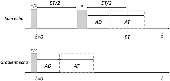
FIGURE 1. pulse sequences used for the simulations. ET: echo-time, AD: acquisition delay, AT: acquisition time, and
Hence, the expression for an acquired signal with the 2D spin echo sequence is:
where ΔB (x,y,t) = B (x,y,t)-B0, Gp the phase gradient intensity and τp the phase gradient pulse time. Gr is the read gradient intensity, and t ∈ [0, AT]. z is the slice selection direction, Δz is the slice size and z0 the center of the slice. This equation does not consider the effects that instability could generate during the slice selection process. Under this approximation, the dependence on z can be avoided by considering the projection of the slice in z0. The times associated with the readout pulses were defined as AT/2 before the π pulse, and AT during the signal acquisition. Using the field model of Eq. 3 and Eq. 6 can be rewritten as:
where
According to these equations, the accumulated dephasing (non-refocused spins) due to the magnetic field instability at the echo time is γB0Ip-se. This term can be considered time-independent and is the equivalent to the phase error proposed in reference [48]. Therefore, Ip-se generates defects along the phase encoding direction. Correspondingly, γB0Ir-se is the dephasing generated by the field instability during the signal acquisition. It is time-dependent and affects the read encoding direction (in similarity with the approach made in [47]). It is important to notice that both terms (Ip-se and Ir-se) are multiplied by B0, which means that the signal is more sensitive to the instability at high fields.
On the other hand, the signal in a 2D gradient echo sequence can be written as:
where
Here, γB0Ip-ge is the accumulated dephasing due to the magnetic field instability in the middle of the acquisition window. In contrast with the spin-echo sequence, the integral has the same sign at any instant. It can be considered time-independent and, as a consequence, generates defects along the phase encoding direction. In contrast, the dephasing generated by the instability during the signal acquisition is γB0Ir-ge. It is time-dependent and affects the readout encoding direction. It is important to note that in this case the magnetic field inhomogeneity generates artifacts in both encoding directions. This is a key-difference between both sequences: in the spin-echo sequence the inhomogeneity only affects the readout encoding direction. In contrast, in the gradient-echo sequence the inhomogeneity is never refocused, thus increasing the undesired effects in the images. As well as for the SE, both terms (Ip-ge and Ir-ge) are multiplied by B0. That is, the signal is more sensitive to the instability at high fields.
In order to analyze the described effects on the signals we have simulated instabilities with two different characteristics: random fluctuations of the magnetic field, and including a dominant frequency component. These two cases represent the main sources of instabilities usually present in the associated instrumentation. Either random noise originated in the electronics (thermal noise, shot, flicker and transit time noises originated in semiconductor devices, and other), or unfiltered low-frequency components (typical harmonics from the power line or originated in the power electronics), and/or high-frequency radio signals that resonate, couples or interferes with the instrument electronics.
For both cases, ΔC (x,y) was simulated using a random surface rsgeng2D (http://www.mysimlabs.com). This function generates a 2D matrix that was previously tested in diverse areas [53, 54]. The algorithm allows for changing the correlation length between matrix components in both directions (rows and columns). ΔC (x,y) has the same matrix size as the image, and each element corresponds to a position in the space. As the inhomogeneity is expected to be smooth, the correlation parameter was fixed at 0.5 (it can vary from 0 to 1) in both directions.
The degradation of the image quality was calculated as a function of the ET for both cases. In order to simplify calculations, the slice selection process was neglected, and the images were simulated as 2D projection images. As mentioned above,
For all the simulations, we fixed the maximum gradient amplitudes at 45 mT/m. The main magnetic field was fixed at 0.125 T, the maximum inhomogeneity was fixed at 1,400 ppm (representative of the measured value within the volume of interest, VOI, in our experiments) and the instability at 220 ppm (with a simulation timescale that is consistent with the acquired signal duration), in accordance with the characteristics of our homemade prototype [35]. The simulations were performed without adding noise, that is, the whole signal comes from the sample. In addition, the gradient fields were assumed to be perfectly linear, and concomitant fields were not considered.
The simulations were performed in Matlab and processed on an Intel Core i7-8565U CPU with a processor base frequency of 1.8 GHz.
To characterize more precisely how the instability affects the images acquired through these two pulse sequences, we have simulated images with stabilities from 50 ppm to 1,200 ppm. In addition, a quantitative parameter was defined as the sum of the pixels outside of the reference image (ORI). Thus, the ORI is zero for the ideal reference image. If the image becomes distorted or we have ghosting due to magnetic field instability, non-zero signal intensity will appear in the region corresponding to the dark portion of the reference image. In this case the ORI becomes nonzero. Simulations were repeated 32 times for each instability value, and the ORI signal intensity was averaged to avoid any abnormal behavior due to the random instability.
The two bright circles of the reference image represent, for example, two tubes filled with water. This means that the total signal intensity of the image must be independent of the image distortion induced by magnetic field instability. In other words, an image distortion can be thought as a signal spreading outside the region defined by the bright circles, i.e., into the dark region corresponding to the reference image (which emulates the situation of an image acquired with perfect magnetic field homogeneity and stability).
Finally, we analyzed the effect of the echo time duration in the SEs. We fixed the instability to 220 ppm, varied the echo time from 1 ms to 21 ms, and calculated the average signal intensity in the ORI over 32 simulations.
In this subsection, the instability is simulated as a pure harmonic component where each acquisition starts with a random phase ϕ:
The maximum amplitude A was fixed at 220 ppm; thus, the instability will be a sinusoidal function oscillating between ±220 ppm. This represents a high instability considering that cryogenic magnets can be stabilized to values lower than 1 part-per-billion [55].
Simulations were only performed for the SEs. Firstly, we simulated images with instabilities with the main frequency in the range of 0–2 kHz for three different echo times (ET = 1 ms, 2 ms and 4 ms), and calculated the mean signal in the ORI. Then, we performed simulations with instabilities with frequencies in the range of 0–20 kHz and for four echo times (ET = 1 ms, 2 ms, 4 ms, and 16 ms).
Finally, we simulated three images: perfect conditions (reference), and then two images with different echo times (38 ms and 40 ms) and same instability with a main frequency of 50 Hz (typical frequency instability induced by the electric line). We specifically chose 40 ms as echo time because ET/2 is exactly one frequency period.
We present two experiments to demonstrate the correct behavior of our model and simulations. The first experiment consisted of measuring FID signals under different magnetic field homogeneities. The second one consisted of acquiring 2D fast-field-cycling (FFC) MRI images in our home-made prototype under different echo times. This last experiment allows determining the nature of the dominant instability affecting the images (random noise or dominant frequency). This information turns relevant to delineate the best method to minimize the artifacts.
The following experiment was aimed to check the predictions suggested by the proposed model. FID signals were acquired with one scan, two scans, and four scans under different magnetic field homogeneities (90 ppm, 250 ppm, and 370 ppm). Hence, if the signals are immune to the instability, they can be accumulated (or averaged) reducing the white noise without signal loss. That is, the only difference related to thenumber of scans must be the SNR.
The experiment was performed in a commercial Stelar Spinmaster FC-2000/C/D (Mede, Italy) relaxometer. The magnetic field homogeneity was changed by relocating the probe (sample) in the magnet away from the central region (maximal homogeneity). The sample was deionized water with 4.5 mm of height in a standard 10 mm diameter test tube. The pulse sequence was a non-polarized (NP) sequence [42], with a polarization and detection field of 0.375 T (15 MHz in terms of proton Larmor frequency). The receptor bandwidth was set to 40 kHz and the acquisition window 4.5 ms.
Images were acquired with different echo times in a homemade MRI-relaxometer with magnetic field instability of 220 ppm/s and inhomogeneity of 1,400 ppm within a VOI of the order of 35 cm3 [35]. The instability was measured from the standard deviation of the frequency shifts of the peak value of the Fourier transform (FT) of the echo signal (acquired without gradients, 50 samples acquired consecutively). The pulse sequence was a non-polarized (NP) sequence [42] with a relaxation and detection field of 0.125 T (5 MHz in terms of proton Larmor frequency). The image acquisition was based on a spin-echo sequence with hard RF pulses, an irradiation bandwidth of 100 kHz andan acquisition window of 1,024 µs. Six images with echo times from 2 ms to 11.1 ms were acquired. Images were acquired without slice selection to maximize the SNR. The sample was a 25 mM solution of deionized water (18 MΩ/cm, milli-Q purification system Osmion 5, Apema, Villa Dominico, Buenos Aires, Argentina) and copper sulfate (Ciccarelli, San Lorenzo, Santa Fé, Argentina).
Figure 2 shows simulated images for a GEs with N = 64, AD = 0.5 ms and AT = 1 ms. Figure 2A shows the reference image (perfect homogeneity and stability). Figure 2B corresponds to the image affected by both instability and inhomogeneity. Figure 2C the image under effects of inhomogeneity only (
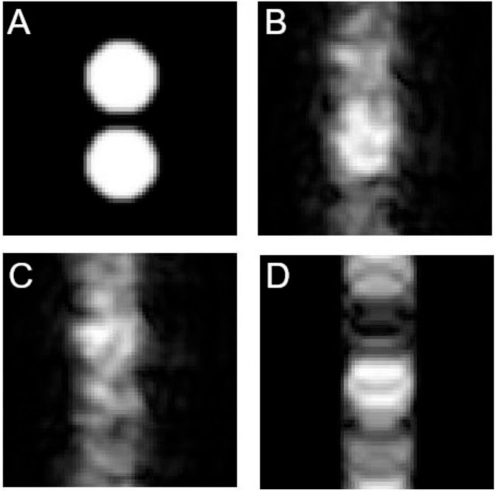
FIGURE 2. Simulated images with gradient-echo sequence. The vertical direction corresponds to the phase encoding direction. (A) Reference image, (B) Degraded by both inhomogeneity and instability, (C) Degraded by inhomogeneity, (D) Degraded by instability. N = 64, AD = 0.5 ms and AT = 1 ms.
Figure 3C shows images simulated for a SEs with ET = 2 ms and AT = 1 ms. As in the previous case, A: reference, B: dual degradation, C: inhomogeneity only and D: instability only.
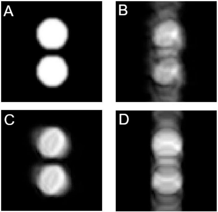
FIGURE 3. Simulated images with spin-echo sequence. The vertical direction corresponds to phase encoding. (A) Reference image, (B) Degraded by both inhomogeneity and instability, (C) Degraded by inhomogeneity, (D) Degraded by instability. N = 64, ET = 2 ms and AT = 1 ms.
Figure 4 shows the ORI signal intensity as a function of the magnetic field instability from 50 ppm to 1200 ppm. Due to the random nature of the instability, each point in the curve wasobtained by averaging 32 images. The associated uncertainty to each point is the standard deviation of the mean value after considering a coverage factor of 95%. The total intensity of each image was normalized to 1, so the calculated ORI is proportional to the percentage of signal spread outside thebright circles. The ORI signal is zero for the reference image and is thus not shown in Figure 4. For a highly degraded image, where the signal intensity is homogeneously spread along the phase direction, the ORI intensity approaches 0.5. That is, this is the expected maximum for a totally degraded image. In fact, the bright circles occupy 50.7% of the image area along the phase direction. Thus, in the case the net signal intensity of the circles becomes homogeneously spread along the phase direction, the theoretical value of the ORI in this example is 0.493.
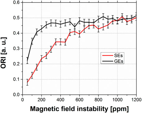
FIGURE 4. signal intensity ORI vs. magnetic field instability. The black curve is associated with the GEs and the red with SEs.
In Figure 4, the signal intensity ORI in the GEs is greater than in SEs until a stability of 1,000 ppm, where the results from both sequences are undistinguishable. The GEs saturate rapidly to values close to 0.5, showing a great sensitivity to instability variations (between 0 ppm and 250 ppm). On the other hand, the SEs is more robust, saturating at instabilities of 1,000 ppm.
Figure 5 shows the effect of the echo time duration in the SEs for a fixed instability to 220 ppm, within an echo time range from 1 ms to 21 ms. As in the previous case, the average ORI signal intensity results from 32 simulations. This plot suggests that short echo times are preferable to avoid image degradation due to instability.
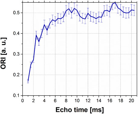
FIGURE 5. ORI signal intensity as a function of ET in images simulated through SEs, for a fixed instability to 220 ppm.
Figure 6 shows the ORI signal intensity dependence on the main frequency of the instability in the range from 0 to 2 kHz for three different echo times (ET = 1 ms, 2 ms, and 4 ms). As can be observed, when the frequency associated with ET/2 is proportional to the instability frequency, the ORI signal intensity becomes minimized. In other words, when an integer number of cycles fits ET/2, each term of Ir-se is null, and, consequently, the ORI signal is minimal (see Figure 7). Furthermore, each minimum has an associated bandwidth, showing that the pulse sequences work as a filter. In addition, the bandwidth increases at higher frequencies (see Figure 6, ET = 4 ms). However, the ORI is not equal to 0 because Ir-se is always nonzero. Figure 8 shows how critical is the choice of the echo time is SEs experiment to avoid ghosting in the image due to monochromatic instability.

FIGURE 6. Signal intensity ORI as function of the instability frequency. Images simulated for SEs. Left: ET = 1 ms, middle: ET = 2 ms and right: ET = 4 ms. The uncertainty of each point is not shown for a clear interpretation of the curve’s behaviors, but it is represented in the variability of the dataset.
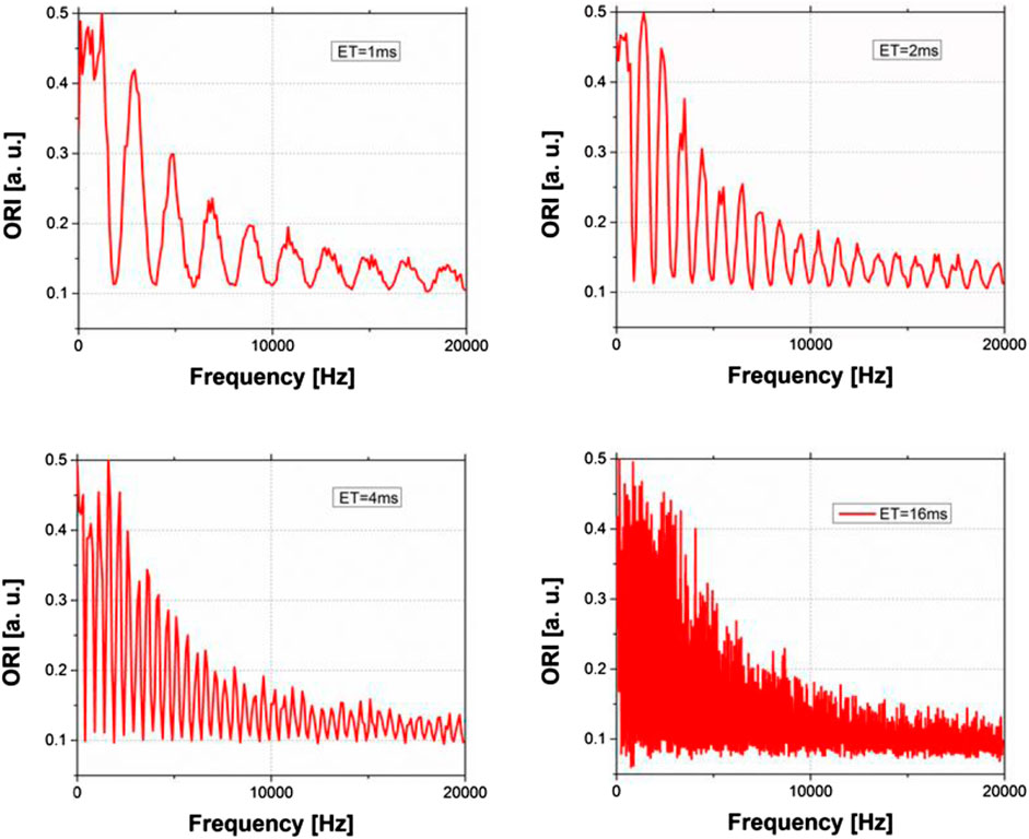
FIGURE 7. Signal intensity ORI as function of the instability frequency. Images simulated for SEs. Top left: ET = 1 ms, top right: ET = 2 ms, bottom left: ET = 4 ms and bottom right: ET = 16 ms.
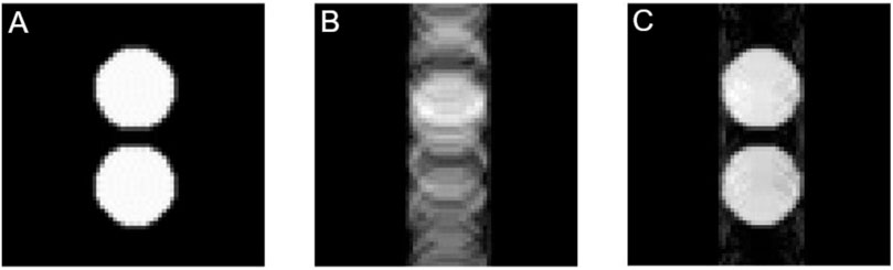
FIGURE 8. Simulated images with SEs. (A) Reference image. (B) Image with frequency instability of 50 Hz and ET = 38 ms. (C) Image with frequency stability of 50 Hz and ET = 40 ms.
Figure 9 shows the NMR signal magnitudes and its Fourier Transform (FT). The FID signals magnitude acquired with 1, 2, and 4 scans are indistinguishable, independently of the magnetic field inhomogeneity, for a stability of 35 ppm. This is consistent withequation 4, and shows that the signal magnitude is unaltered by the magnetic field instability. However, the increase of the magnetic field inhomogeneity leads to a decrease of the signal amplitude and length. On the other hand, the FT is sensitive to phase changes in the NMR signal, which means that it is not immune to magnetic field instability. The FT of the signals acquired with an inhomogeneity of 90 ppm shows that there is a high variability between the spectra obtained after 1, 2, and 4 scans, even for a field stability of 35 ppm. At 250 ppm of inhomogeneity, the differences between the signals are smaller, while for 370 ppm are practically indistinguishable. Consequently, this simple experiment evidences a direct relationship between the instability immunity and the magnetic field inhomogeneity in an FID experiment. Furthermore, it agrees with Eq. (5), experimentally proving that the model is accurate to describe and understand the influence of magnetic field instability and inhomogeneity in NMR experiments.
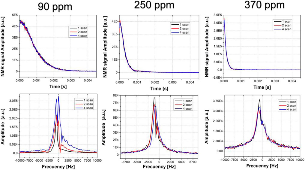
FIGURE 9. NMR signal amplitudes (top) and its FT (bottom) acquired under 90 ppm (left), 250 ppm (middle) and 370 ppm (right) with 1 scan (black line), 2 scans (red line), and 4 scans (blue line). The mean value of the field instability was 35 ppm.
Figure 10 shows the image acquired in our MRI relaxometer. The artifacts increase drastically with the echo time suggesting that the dominant component of the instability is originated in random fluctuations.
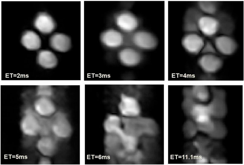
FIGURE 10. Images acquired with different echo times. Image parameters: size 64 × 64, Gr = 54.9 mT/m, Gp = 71.3 mT/m, 2 scans and 1 dummy.
In this manuscript we have presented a simple model to describe the effects of the magnetic field inhomogeneity and instability in MRI. The model could successfully explain the observed behavior of FID signals acquired with different inhomogeneities in a commercial relaxometer. A key feature of the presented experiments and simulations is that a correlation between the magnetic field inhomogeneity and the signal immunity due to the instability can be established. However, this behavior does not replicate in MRI, where a more complex situation holds. The pulse gradients and the k-space sampling broke this correlation due to the creation of a second dimension.
It is worth noting that spins dephasing accumulation in both phase and readout encoding directions, γB0Ip-se and γB0Ir-se, are proportional to the magnetic field strength B0. This feature suggests a higher natural immunity to magnetic field instability at low-field conditions, thus representing an additional motivation for pre-polarized MRI schemes. That is, magnetization boosted-up with a polarization B0 pulse, followed by an MRI sequence applied at a lower field. In any case the result holds valid for fixed-field MRI systems operating at low field conditions. On the other side, this result prevents the use of electromagnets for magnetic field strengths were, due to associated costs and technical difficulties, they would not be the best option anyway.
As it is possible to observe in Figures 2, 3, simulated images for the GEs are highly degraded, while the images with SEs show a higher robustness to magnetic field instabilities. The main difference relies on the effect of the magnetic field inhomogeneity. The GEs generate artifacts along both encoding directions, leading to frequency shifts. Moreover, the dephasing induced by the inhomogeneity is accumulated all the time during GEs, while in the SEs, the magnetization is re-focused due to the presence of a π pulse [56]. Nonetheless, in the GEs the defects are also highlighted in the case of images degraded only by the stability. The GEs accumulate the dephasing of the low-frequency instabilities, an undesirable effect that can be avoided by using the SEs.
The results from Figure 4 are consistent with the simulations showed in Figures 2, 3, highlighting the importance of the low-frequency re-focusing. Therefore, the spin-echo sequence is the recommended sequence to minimize instability-induced image distortions and ghosting.
Instabilities with different characteristics were described. The first one considers the instability as a random fluctuation, where the magnetic field between scans is less correlated than during a single scan. The second one approximates the instability as a monochromatic harmonic fluctuation with random phase between scans. Different strategies are to be considered to minimize the effects induced by these two kinds of instability. While for random instability the best strategy relies on minimizing the echo time, for a monochromatic instability, the best strategy consists of selecting an echo time in which a complete cycle of the instability is contained in ET/2. As expected, a realistic experimental situation may have both contributions. Therefore, a compromise relationship is presented, that is, the echo time that minimize random fluctuations should fit a proper value in order to cancel a dominant monochromatic component, if any.
Experimental images with different echo times were acquired in our MRI relaxometer, showing a strong correlation between the ET and the image degradation. This result shows that in the moment of the experiment, the instability of the magnetic field of the machine was mainly of random nature. A concluding remark from these results is that short echo times seem to be preferable in case of random magnetic field fluctuations.
In this work, we have shown that the study of the nature of the instability is a fundamental point to find the best strategy to minimize instability artifacts. Furthermore, if a pick-up coil or sensors are implemented to measure
The raw data supporting the conclusion of this article will be made available by the authors, without undue reservation.
GR performed the simulations, realized experimental work and wrote the manuscript. CS conceptualized the method and wrote the manuscript. EA conceptualized the method, realized experimental work and wrote the manuscript. All authors contributed to the article and approved the submitted version.
The author(s) declare financial support was received for the research, authorship, and/or publication of this article. This work was funded by FONCYT project number PICT-2017–2195 and CONICET PIP 2021–2013 11220200102521CO. Support from Secyt-UNC is also acknowledged.
GR acknowledges CONICET for the postdoctoral fellowship during this work.
The authors declare that the research was conducted in the absence of any commercial or financial relationships that could be construed as a potential conflict of interest.
All claims expressed in this article are solely those of the authors and do not necessarily represent those of their affiliated organizations, or those of the publisher, the editors and the reviewers. Any product that may be evaluated in this article, or claim that may be made by its manufacturer, is not guaranteed or endorsed by the publisher.
1. Marques JP, Simonis FFJ, Webb AG. Low-field MRI: an MR physics perspective. J Magn Reson Imaging (2019) 49:1528–42. doi:10.1002/jmri.26637
2. Sarracanie M, Salameh N. Low-field MRI: how low can we go? A fresh view on an old debate. Front Phys (2020) 8:1–14. doi:10.3389/fphy.2020.00172
3. Anoardo E, Rodriguez GG. New challenges and opportunities for low-field MRI. J Magn Reson Open (2023) 14-15:100086. doi:10.1016/j.jmro.2022.100086
4. O’Reilly T, Teeuwisse WM, de Gans D, Koolstra K, Webb AG. In vivo 3D brain and extremity MRI at 50 mT using a permanent magnet Halbach array. Magn Reson Med (2020) 85:495–505. doi:10.1002/mrm.28396
5. Sarracanie M, Lapierre C, Salameh N, Waddington DEJ, Witzel T, Rosen MS. Low-cost high-performance MRI. Sci Rep (2015) 5:15177–9. doi:10.1038/srep15177
6. Nakagomi M, Kajiwara M, Matsuzaki J, Tanabe K, Hoshiai S, Okamoto Y, et al. Development of a small car-mounted magnetic resonance imaging system for human elbows using a 0.2 T permanent magnet. J Magn Reson (2019) 304:1–6. doi:10.1016/j.jmr.2019.04.017
7. Waddington DEJ, Boele T, Maschmeyer R, Kuncic Z, Rosen MS. High-sensitivity in vivo contrast for ultra-low field magnetic resonance imaging using superparamagnetic iron oxide nanoparticles. Sci Adv (2020) 6:eabb0998–10. doi:10.1126/sciadv.abb0998
8. Wald LL, McDaniel PC, Witzel T, Stockmann JP, Cooley CZ. Low-cost and portable MRI. J Magn Reson Imaging (2019) 52:686–96. doi:10.1002/jmri.26942
9. Cooley CZ, McDaniel PC, Stockmann JP, Srinivas SA, Cauley SF, Śliwiak M, et al. A portable scanner for magnetic resonance imaging of the brain. Nat Biomed Eng (2020) 5:229–39. doi:10.1038/s41551-020-00641-5
10. Guallart-Naval T, Algarín JM, Pellicer-Guridi R, Galve F, Vives-Gilabert Y, Bosch R, et al. Portable magnetic resonance imaging of patients indoors, outdoors and at home. Sci Rep (2022) 12:13147. doi:10.1038/s41598-022-17472-w
11. Coffey AM, Truong ML, Chekmenev EY. Low-field MRI can be more sensitive than high-field MRI. J Magn Reson (2013) 237:169–74. doi:10.1016/j.jmr.2013.10.013
12. Hoult DI, Richards RE. The signal-to-noise ratio of the nuclear magnetic resonance experiment. J Magn Reson (1976) 24:71–85. doi:10.1016/0022-2364(76)90233-X
13. Broche LM, Ross PJ, Davies GR, MacLeod MJ, Lurie DJ. A whole-body Fast Field-Cycling scanner for clinical molecular imaging studies. Sci Rep (2019) 9:10402. doi:10.1038/s41598-019-46648-0
14. Edelstein WA, Glover GH, Hardy CJ, Redington RW. The intrinsic signal-to-noise ratio in NMR imaging. Magn Reson Med (1986) 3:604–18. doi:10.1002/mrm.1910030413
15. Matter NI, Scott GC, Grafendorfer T, Macovski A, Conolly SM. Rapid polarizing field cycling in magnetic resonance imaging. IEEE Trans Med Imag (2006) 25:84–93. doi:10.1109/tmi.2005.861014
16. McDermott R, Lee S, Haken B, Trabesinger AH, Pines A, Clarke J. Microtesla MRI with a superconducting quantum interference device. PNAS (2004) 21:7857–61. doi:10.1073/pnas.0402382101
17. Dong H, Zhang Y, Krause H-J, Xie X, Offenhäusser A. Low field MRI detection with tuned HTS SQUID magnetometer. IEEE Trans Appl Supercon (2011) 21:509–13. doi:10.1109/tasc.2010.2091713
18. Demachi K, Hayashi K, Adachi S, Tanabe K, Tanaka S. T1-weighted image by ultra-low field SQUID-MRI. IEEE Trans Appl Supercon (2019) 29:1–5. doi:10.1109/TASC.2019.2902772
19. Suefke M, Liebisch A, Blümich B. External high-quality-factor resonator tunes up nuclear magnetic resonance. Nat Phys (2015) 11:767–71. doi:10.1038/nphys3382
20. Jouda M, Kamberger R, Leupold J, Spengler N, Henning J, Gruschke O, et al. A comparison of Lenz lenses and LC resonators for NMR signal enhancement. Concepts Magn Reson B (2018) 47b:e21357. doi:10.1002/cmr.b.21357
21. Zhang Y, Guo Y, Kong X, Zeng P, Yin H, Wu J, et al. Improving local SNR of a single-channel 54.6 mT MRI system using additional LC-resonator. J Magn Reson (2022) 339:107215. doi:10.1016/j.jmr.2022.107215
22. Sarracanie M. Fast quantitative low-field magnetic resonance imaging WithOPTIMUM—optimized magnetic resonance fingerprinting using a stationary steady-state cartesian approach and accelerated acquisition schedules. Invest Radiol (2022) 57:263–71. doi:10.1097/RLI.0000000000000836
23. Lehmkuhl S, Fleischer S, Lohmann L, Rosen MS, Chekmenev EY, Adams A, et al. RASER MRI: magnetic resonance images formed spontaneously exploiting cooperative nonlinear interaction. Sci Adv (2022) 8:eabp8483. doi:10.1126/sciadv.abp8483
24. Aja-Fernández S, Vegas-Sánchez-Ferrero G. The problem of noise in MRI. In: Statistical analysis of noise in MRI. Berlin, Germany: Springer (2016). doi:10.1007/978-3-319-39934-8_1
25. Koonjoo N, Zhu B, Bagnall GC, Bhutto D, Rosen MS. Boosting the signal-to-noise of low-field MRI with deep learning image reconstruction. Sci Rep (2021) 11:8248. doi:10.1038/s41598-021-87482-7
26. Araya YT, Martínez-Santiesteban F, Handler WB, Harris CT, Chronik BA, Scholl TJ. Nuclear magnetic relaxation dispersion of murine tissue for development of T1 (R1) dispersion contrast imaging. NMR Biomed (2017) 30:e3789. doi:10.1002/nbm.3789
27. Gossuin Y, Gillis P, Hocq A, Vuong QL, Roch A. Magnetic resonance relaxation properties of superparamagnetic particles. Wiley Interdiscip Rev Nanomedicine Nanobiotechnology (2009) 1:299–310. doi:10.1002/wnan.36
28. Yin X, Russek SE, Zabow G, Sun F, Mohapatra J, Keenan KE, et al. Large T1 contrast enhancement using superparamagnetic nanoparticles in ultra-low field MRI. Sci Rep (2018) 8:11863. doi:10.1038/s41598-018-30264-5
29. Hendrick RE, Haacke EM. Basic physics of MR contrast agents and maximization of image contrast. J Magn Reson Imaging (1993) 3:137–48. doi:10.1002/jmri.1880030126
30. Rabbani H, Nezafat R, Gazor S. Wavelet-domain medical image denoising using bivariate Laplacian mixture model. IEEE Trans Biomed Eng (2009) 56:2826–37. doi:10.1109/TBME.2009.2028876
31. Ippoliti M, Adams LC, Winfried B, Hamm B, Spincemaille P, Wang Y, et al. Quantitative susceptibility mapping across two clinical field strengths:contrast-to-noise ratio enhancement at 1.5T. J Magn Reson Imaging (2018) 48:1410–20. doi:10.1002/jmri.26045
32. Epstein CL. Magnetic resonance imaging in inhomogeneous fields. Inverse Probl (2004) 20:753–80. doi:10.1088/0266-5611/20/3/007
33. Kim JK, Plewes DB, Henkelman RM. Magnetic resonance imaging in an inhomogeneous magnetic field. US Patent (1994):5309101.
34. Perlo J, Casanova F, Blümich B. 3D imaging with a single-sided sensor: an open tomograph. J Magn Reson (2004) 166:228–35. doi:10.1016/j.jmr.2003.10.018
35. Romero JA, Rodriguez GG, Anoardo E. A fast field-cycling MRI relaxometer for physical contrasts design and pre-clinical studies in small animals. J Magn Reson (2020) 311:106682. doi:10.1016/j.jmr.2019.106682
36. Vovk U, Pernuš F, Likar B. A review of methods for correction of intensity inhomogeneity in MRI. IEEE Trans Med Imaging (2007) 26:405–21. doi:10.1109/TMI.2006.891486
37. Rodriguez GG, Salvatori A, Anoardo E. Dual k-space and image-space post-processing for field-cycling MRI under low magnetic field stability and homogeneity conditions. Magn Reson Imag (2022) 87:157–68. doi:10.1016/j.mri.2022.01.008
38. Koolstra K, O’Reilly T, Börnert P, Webb A. Image distortion correction for MRI in low field permanent magnet systems with strong B0 inhomogeneity and gradient field nonlinearities. MAGMA (2021) 34:631–42. doi:10.1007/s10334-021-00907-2
39. Lother S, Schiff SJ, Neuberger T, Jakob PM, Fidler F. Design of a mobile, homogeneous, and efficient electromagnet with a large field of view for neonatal low-field MRI. Magn Reson Mater Phys Biol. Med. (2016) 29:691–8. doi:10.1007/s10334-016-0525-8
40. Michal CA. Low-cost low-field NMR and MRI: instrumentation and applications. J Magn Reson (2020) 319:106800. doi:10.1016/j.jmr.2020.106800
41. Kimmich R, Anoardo E. Field-cycling NMR relaxometry. Prog NMR Sepctrosc (2004) 44:257–320. doi:10.1016/j.pnmrs.2004.03.002
42. Anoardo E, Galli G, Ferrante G. Fast-field-cycling NMR: applications and instrumentation. Appl Magn Reson (2001) 20:365–404. doi:10.1007/BF03162287
43. Lurie DJ, Hutchison JMS, Bell LH, Nicholson I, Bussell DM, Mallard JR. Field-cycled proton-electron double-resonance imaging of free radicals in large aqueous samples. J Magn Reson (1989) 84:431–7. doi:10.1016/0022-2364(89)90392-2
44. Ungersma SE, Matter NI, Hardy JW, Venook RD, Macovski A, Conolly SM, et al. Magnetic resonance imaging with T1 dispersion contrast. Magn Reson Med (2006) 55:1362–71. doi:10.1002/mrm.20910
45. Rodriguez GG, Erro EM, Anoardo E. Fast iron oxide-induced low-field magnetic resonance imaging. J Phys D: Appl Phys (2020) 54:025003. doi:10.1088/1361-6463/abbe4d
46. Rodriguez GG, Anoardo E. Proton double irradiation field-cycling nuclear magnetic resonance imaging: testing new concepts and calibration methods. IEEE Trans Instrum Meas (2021) 70:1–8. doi:10.1109/TIM.2020.3037304
47. Morgan P, Conolly S, Scott G, Macovski A. A readout magnet for prepolarized MRI. Magn Reson Med (1996) 36:527–36. doi:10.1002/mrm.1910360405
48. Bödenler M, Rochefort L, Ross PJ, Chanet N, Guillot G, Davies GR, et al. Comparison of fast field-cycling magnetic resonance imaging methods and future perspectives. Mol Phys (2019) 117:832–48. doi:10.1080/00268976.2018.1557349
49. Broche LM, Ross PJ, Davies GR, Lurie DJ. Simple algorithm for the correction of MRI image artefacts due to random phase fluctuations. Magn Reson Imaging (2017) 44:55–9. doi:10.1016/j.mri.2017.07.023
50. Atkinson D, Hill DLG, Stoyle PNR, Summers PE, Keevil SF. Automatic correction of motion artifacts in magnetic resonance images using an entropy focus criterion. IEEE Trans Med Imaging (1997) 16:903–10. doi:10.1109/42.650886
51. Atkinson D, Hill DLG, Stoyle PNR, Summers PE, Clare S, Bowtell R, et al. Automatic compensation of motion artifacts in MRI. Magn Reson Med (1999) 41:163–70. doi:10.1002/(SICI)1522-2594(199901)41:1<163::AID-MRM23>3.0.CO;2-9
52. Bernstein MA, King KF, Joe Zhou X. Handbook of MRI pulse sequences. Amsterdam: Elsevier Academic Press (2007). doi:10.4314/bcse.v21i3.21211
53. Javili A, McBride A, Steinmann P, Reddy BD. A unified computational framework for bulk and surface elasticity theory: a curvilinear-coordinate-based finite element methodology. Comput Mech (2014) 54:745–62. doi:10.1007/s00466-014-1030-4
54. Ye M, Feng P, Li Y, Wang D, He Y, Cui W. The total secondary electron yield of a conductive random rough surface. J Appl Phys (2019) 125:043301. doi:10.1063/1.5023769
55. Takeda Y, Maeda H, Ohki K, Yanagisawa Y. Review of the temporal stability of themagnetic field for ultra-high field superconducting magnets with aparticular focus on superconducting joints between HTS conductors. Supercond Sci Technol (2022) 35:043002. doi:10.1088/1361-6668/ac5645
57. Liu Y, Leon ATL, Zhao Y, Xiao L, Mak HKF, Tsang ACO, et al. A low-cost and shielding-free ultra-low-field brain MRI scanner. Nat Commun (2021) 12:7238. doi:10.1038/s41467-021-27317-1
Keywords: low-field, field instability, MRI, electromagnets, field inhomogeneity
Citation: Rodriguez GG, Schürrer CA and Anoardo E (2023) Low-field MRI at high magnetic field instability and inhomogeneity conditions. Front. Phys. 11:1249771. doi: 10.3389/fphy.2023.1249771
Received: 29 June 2023; Accepted: 18 October 2023;
Published: 02 November 2023.
Edited by:
Fangrong Zong, Beijing University of Posts and Telecommunications (BUPT), ChinaReviewed by:
Per Magnelind, Los Alamos National Laboratory (DOE), United StatesCopyright © 2023 Rodriguez, Schürrer and Anoardo. This is an open-access article distributed under the terms of the Creative Commons Attribution License (CC BY). The use, distribution or reproduction in other forums is permitted, provided the original author(s) and the copyright owner(s) are credited and that the original publication in this journal is cited, in accordance with accepted academic practice. No use, distribution or reproduction is permitted which does not comply with these terms.
*Correspondence: Esteban Anoardo, ZWFub2FyZG9AdW5jLmVkdS5hcg==; Gonzalo G. Rodriguez, Z29uemFsb2dhYnJpZWwucm9kcmlndWV6QG1waW5hdC5tcGcuZGU=
†Present address: Gonzalo G. Rodriguez, NMR Signal Enhancement Group, Max Planck Institute for Multidisciplinary Sciences, Göttingen, Germany
Disclaimer: All claims expressed in this article are solely those of the authors and do not necessarily represent those of their affiliated organizations, or those of the publisher, the editors and the reviewers. Any product that may be evaluated in this article or claim that may be made by its manufacturer is not guaranteed or endorsed by the publisher.
Research integrity at Frontiers
Learn more about the work of our research integrity team to safeguard the quality of each article we publish.