Fractional stochastic vibration system under recycling noise

The fractional stochastic vibration system is quite different from the traditional one, and its application potential is enormous if the noise can be deployed correctly and the connection between the fractional order and the noise property is unlocked. This article uses a fractional modification of the well-known van der Pol oscillator with multiplicative and additive recycling noises as an example to study its stationary response and its stochastic bifurcation. First, based on the principle of the minimum mean square error, the fractional derivative is equivalent to a linear combination of damping and restoring forces, and the original system is simplified into an equivalent integer order system. Second, the Itô differential equations and One-dimensional Markov process are obtained according to the stochastic averaging method, using Oseledec multiplicative ergodic theorem and maximal Lyapunov exponent to judge local stability, and judging global stability is done by using the singularity theory. Lastly, the stochastic D-bifurcation behavior of the model is analyzed by using the Lyapunov exponent of the dynamical system invariant measure, and the stationary probability density function of the system is solved according to the FPK equation. The results show that the fractional order and noise property can greatly affect the system’s dynamical properties. This paper offers a profound, original, and challenging window for investigating fractional stochastic vibration systems.

1 Introduction

Fractional derivative [1, 2] is an extension of the theory of integer derivatives, and the study of fractional derivatives has a history of over 300 years. Some new materials have appeared, e.g., viscoelastic materials, nanomaterials, cement mortar, 3D-printed materials, and porous materials [3–8], which are different from either a solid or a fluid, and their constitutive relation is extremely difficult to be expressed correctly by the traditional calculus though much effort has been made to solve the problem, for example, using the fractal viscoelastic model [9] and the fractal rheological model [10]; the intractable constitutive relation has not yet been solved.

Considering its memory property, we consider that fractional calculus might be the best candidate for stochastic dynamical systems [11, 12]. Stochastic disturbances are widespread in nature, and fractional stochastic systems have become a hot spot in both mathematics and physics to deal with noise excitation. For example, energy-harvesting devices [13–15] are always subject to random excitation, and a fractional model can effectively reveal the bifurcation properties and multiple attractors of the energy-harvesting system, for example, Ref. [16]. Fractional models for Gaussian white noise also caught much attention [17–21], and the fractional convolution kernel neural network is a suitable mathematical tool for fault diagnosis [22–24]. Duffing oscillator [25, 26] is extended to its fractional partner under noise [27, 28]. Van der Pol oscillator [29] is another widely used model for the analysis of fractional stochastic P-bifurcation [30, 31].

In reality, noise exists in all aspects of practical applications, especially in nonlinear systems. The properties of stationary response, energy-harvesting efficiency, stability, and bifurcation will be greatly affected by noise excitation. At present, the research on the dynamic behavior of systems driven by recycling noise has attracted widespread attention from domestic and foreign scholars and achieved fruitful results, especially in the birhythmic biological system [32], stochastic resonance in asymmetric bistable systems [33], and the double entropic stochastic resonance phenomenon [34]. In this article, the fractional van der Pol model with recycling noise is adopted to investigate its dynamical properties.

2 Model description

Balthazar van der Pol is a famous electronic engineer in the Netherlands. In 1927, he first deduced the famous van der Pol equation in order to describe the oscillation effect of triodes in electronic circuits, as shown below:

$\ddot{x}-\mu \left(1-x^2\right)\dot{x}+x=0$

Afterward, as a classic nonlinear dynamic system, it is often used in mathematics and some nonlinear dynamic systems to demonstrate its dynamic behavior characteristics. In continuous research, the highest number of nonlinear terms considered is also constantly increasing, and there are also various methods for solving approximate solutions of such equations [35, 36]. From the classical van der Pol equation, changing the order of the equation can obtain systems with different dynamic behaviors, thereby better obtaining the dynamic behavior characteristics of the system. Therefore, we use the following equation to introduce the fractional generalized van der Pol model with multiplicative and additive recycling noise:

$\ddot{x}-\left(-\epsilon +{\alpha }_1{x}^2-{\alpha }_2{x}^4+{\alpha }_3{x}^6-{\alpha }_4{x}^8\right)\dot{x}+{\omega }^{2}x+{}_0{}^c{D}^{p}x={\eta }_1\left(t\right)+x\left(t\right){\eta }_2\left(t\right),(1)$

where $\epsilon$ is the damping coefficient, ${\alpha }_1,{\alpha }_2,{\alpha }_3,{\alpha }_4$ are nonlinear damping coefficients, $\omega$ is the frequency, ${\eta }_1\left(t\right)$ and ${\eta }_2\left(t\right)$ are independent recycling noises, i.e., $D_1\ne D_2$, ${\eta }_i\left(t\right)={\xi }_i\left(t\right)+k{\xi }_i\left(t-\tau \right),\left(i=\mathrm{1,2}\right)$. The power spectral density of recycling noise is obtained as:

$S_i\left(\omega \right)=2D_i\left[1+k^2+2kcos\left(\omega \tau \right)\right],\left(i=1,2\right).(2)$

${}_0{}^c{D}^p\left[x\left(t\right)\right]$ is the Caputo fractional derivative [1, 2] of $p\left(0\le p\le 1\right)$ order about $x\left(t\right)$ defined as:

${}_0{}^c{D}^p\left[x\left(t\right)\right]=\frac{1}{\mathrm{\Gamma }\left(m-p\right)}{\int }_0^t\frac{x^{\left(m\right)}\left(u\right)}{{\left(t-u\right)}^{1+p-m}}du,m-1<p\le m,m\in N.(3)$

There are other definitions of fractional derivatives, for example, two-scale fractal derivative [37–41] and He’s fractional derivative [42]. The Caputo fractional derivative has memory property [43, 44], so it is used for the present study.

The ${}_0{}^c{D}^{p}x$ term in Eq. 1 can be expressed in a combination of spring stiffness and damping terms [45–48], hence, Eq. 1 becomes:

$\ddot{x}-\left(-\epsilon +{\alpha }_1{x}^2-{\alpha }_2{x}^4+{\alpha }_3{x}^6-{\alpha }_4{x}^8+C\left(p\right)\right)\dot{x}$

$+\left({\omega }^2+K\left(p\right)\right)x={\eta }_1\left(t\right)+x\left(t\right){\eta }_2\left(t\right),(4)$

where $C$ and $K$ are the equivalent damping and stiffness coefficients of fractional damping, respectively.

In order to identify $C$ and $K$, we introduce an error function, which reads

$e=-C\left(p\right)\dot{x}+K\left(p\right)x-{}_0{}^c{D}^p\left[x\left(t\right)\right],(5)$

According to the minimum mean square method [44], we have

$\left\{\begin{array}{c}\partial E\left(e^2\right)/\partial \left(C\left(p\right)\right)=0,\\ \partial E\left(e^2\right)/\partial \left(K\left(p\right)\right)=0.\end{array}\right.(6)$

Equation 6 leads to the following equations:

$\left\{\begin{array}{c}E\left[-C\left(p\right){\dot{x}}^2+K\left(p\right)x\dot{x}-\dot{x}{}_0{}^c{D}^{p}x\right]=\underset{T\to \infty }{\lim }\frac{1}{T}{\int }_0^T\left(-C\left(p\right){\dot{x}}^2+K\left(p\right)x\dot{x}-\dot{x}{}_0{}^c{D}^{p}x\right)dt=0,\\ E\left[-C\left(p\right)x\dot{x}+K\left(p\right)x^2-x{}_0{}^c{D}^{p}x\right]=\underset{T\to \infty }{\lim }\frac{1}{T}{\int }_0^T\left(-C\left(p\right)x\dot{x}+K\left(p\right)x^2-x{}_0{}^c{D}^{p}x\right)dt=0.\end{array}\right.(7)$

Assuming that

$x\left(t\right)=a\left(t\right)\mathit{cos}\phi \left(t\right)=a\left(t\right)\mathit{cos}\left(\omega t+\theta \right)(8)$

and $\dot{a}\left(t\right)\approx 0$, we have

$\left\{\begin{array}{c}\dot{x}\left(t\right)=-a\left(t\right)\omega \mathit{sin}\phi \left(t\right),\\ \ddot{x}\left(t\right)=-a\left(t\right){\omega }^2\mathit{cos}\phi \left(t\right).\end{array}\right.(9)$

Considering Eq. 8, 9, we re-write Eq. 7 in the form

$\underset{T\to \infty }{\lim }\frac{1}{T}{\int }_0^T\left(-C\left(p\right){\dot{x}}^2+K\left(p\right)x\dot{x}-\dot{x}{}_0{}^c{D}^{p}x\right)dt$

$=\underset{T\to \infty }{\lim }\frac{1}{T}{\int }_0^T\left(-C\left(p\right)a^2\left(t\right){\omega }^2{\mathit{sin}}^2\phi \left(t\right)-K\left(p\right)a^2\left(t\right)\omega \phi \left(t\right)\mathit{cos}\phi \left(t\right)+a\left(t\right)\omega \mathit{sin}\phi \left(t\right){}_0{}^c{D}^{p}x\right)d\phi$

$\approx -\frac{C\left(p\right)a^2\omega }{2}+\frac{1}{\mathrm{\Gamma }\left(1-p\right)}\underset{T\to \infty }{\lim }\frac{1}{T}{\int }_o^T\left[\left(a\omega \mathit{sin}\phi \right){\int }_0^t\frac{\dot{x}\left(t-\tau \right)}{{\tau }^p}d\tau \right]d\phi$

$=\frac{-C\left(p\right)a^2\omega }{2}-\frac{1}{\mathrm{\Gamma }\left(1-p\right)}\underset{T\to \infty }{\lim }\frac{1}{T}{\int }_0^T{a}^2\omega \mathit{sin}\phi \times \left({\int }_0^t\frac{\mathit{sin}\phi \mathit{cos}\left(\omega \tau \right)-\mathit{cos}\phi \mathit{sin}\left(\omega \tau \right)}{{\tau }^p}d\tau \right)dt=0,$

For the same reason, we have

$\underset{T\to \infty }{\lim }\frac{1}{T}{\int }_0^T\left(-C\left(p\right)x\dot{x}+K\left(p\right)x^2-x{}_0{}^c{D}^{p}x\right)dt$

$=\underset{T\to \infty }{\lim }\frac{1}{T}{\int }_0^T\left(-C\left(p\right)a^2\left(t\right)\omega \mathit{sin}\phi \left(t\right)\mathit{cos}\phi \left(t\right)+K\left(p\right)a^2\left(t\right){\mathit{cos}}^2\phi \left(t\right)-a\left(t\right)\mathit{cos}\phi \left(t\right){}_0{}^c{D}^{p}x\right)d\phi$

$\approx \frac{K\left(p\right)a^2}{2\omega }-\frac{1}{\mathrm{\Gamma }\left(1-p\right)}\underset{T\to \infty }{\lim }\frac{1}{T}{\int }_o^T\left[\left(\mathit{acos}\phi \right){\int }_0^t\frac{\dot{x}\left(t-\tau \right)}{{\tau }^p}d\tau \right]d\phi$

$=\frac{K\left(p\right)a^2}{2\omega }+\frac{1}{\mathrm{\Gamma }\left(1-p\right)}\underset{T\to \infty }{\lim }\frac{1}{T}{\int }_0^T{a}^2\times \mathit{cos}\phi \left({\int }_0^t\frac{\mathit{sin}\phi \mathit{cos}\left(\omega \tau \right)-\mathit{cos}\phi \mathit{sin}\left(\omega \tau \right)}{{\tau }^p}d\tau \right)dt=0.$

Hence

$\left\{\begin{array}{c}\underset{T\to \infty }{\lim }\frac{1}{T}{\int }_0^T\left(-C\left(p\right){\dot{x}}^2+K\left(p\right)x\dot{x}-\dot{x}{}_0{}^c{D}^{p}x\right)dt\\ =\frac{-C\left(p\right)a^2\omega }{2}-\frac{1}{\mathrm{\Gamma }\left(1-p\right)}\underset{T\to \infty }{\lim }\frac{1}{T}{\int }_0^T{a}^2\omega \mathit{sin}\phi \left({\int }_0^t\frac{\mathit{sin}\phi \mathit{cos}\left(\omega \tau \right)-\mathit{cos}\phi \mathit{sin}\left(\omega \tau \right)}{{\tau }^p}d\tau \right)dt=0,\\ \underset{T\to \infty }{\lim }\frac{1}{T}{\int }_0^T\left(-C\left(p\right)x\dot{x}+K\left(p\right)x^2-x{}_0{}^c{D}^{p}x\right)dt\\ =\frac{K\left(p\right)a^2}{2\omega }+\frac{1}{\mathrm{\Gamma }\left(1-p\right)}\underset{T\to \infty }{\lim }\frac{1}{T}{\int }_0^T{a}^2\mathit{cos}\phi \left({\int }_0^t\frac{\mathit{sin}\phi \mathit{cos}\left(\omega \tau \right)-\mathit{cos}\phi \mathit{sin}\left(\omega \tau \right)}{{\tau }^p}d\tau \right)dt=0.\end{array}\right.(10)$

To simplify Eq. 10 further, we use the following asymptotic integrals

$\left\{\begin{array}{c}{\int }_0^t\frac{\mathit{cos}\left(\omega \tau \right)}{{\tau }^p}d\tau ={\omega }^{p-1}\left(\mathrm{\Gamma }\left(1-p\right)\mathit{sin}\left(\frac{p\pi }{2}\right)+\frac{\mathit{sin}\left(\omega t\right)}{{\left(\omega t\right)}^p}\right)+o\left({\left(\omega t\right)}^{-p-1}\right),\\ {\int }_0^t\frac{\mathit{sin}\left(\omega \tau \right)}{{\tau }^p}d\tau ={\omega }^{p-1}\left(\mathrm{\Gamma }\left(1-p\right)\mathit{cos}\left(\frac{p\pi }{2}\right)-\frac{\mathit{cos}\left(\omega t\right)}{{\left(\omega t\right)}^p}\right)+o\left({\left(\omega t\right)}^{-p-1}\right).\end{array}\right.(11)$

In view of Eq. 11, the integral averaging of Eq. 10 with respect to $\phi$ results in

$\left\{\begin{array}{c}C\left(p\right)=-{\omega }^{p-1}\mathit{sin}\left(\frac{p\pi }{2}\right),\\ K\left(p\right)={\omega }^p\mathit{sin}\left(\frac{p\pi }{2}\right).\end{array}\right.(12)$

Hence, the equivalent system (4) can be written in the form

$\ddot{x}-\lambda x+{{\omega }_0}^{2}x={\eta }_1\left(t\right)+x\left(t\right){\eta }_2\left(t\right),(13)$

where

$\left\{\begin{array}{c}\lambda =-\epsilon +{\alpha }_1{x}^2-{\alpha }_2{x}^4+{\alpha }_3{x}^6-{\alpha }_4{x}^8-{\omega }^{p-1}\mathit{sin}\left(\frac{p\pi }{2}\right),\\ {{\omega }_0}^2={\omega }^2+{\omega }^p\mathit{cos}\left(\frac{p\pi }{2}\right).\end{array}\right.(14)$

3 Model processing

Now the problem becomes relatively simple; we assume that the solution of Eq. 13 can be expressed as [49].

$\left\{\begin{array}{c}X=x\left(t\right)=a\left(t\right)\mathit{cos}\mathrm{\Phi }\left(t\right),\\ Y=\dot{x}\left(t\right)=-a\left(t\right){\omega }_0\mathit{sin}\mathrm{\Phi }\left(t\right),\\ \mathrm{\Phi }\left(t\right)={\omega }_{0}t+\theta \left(t\right),\end{array}\right.(15)$

where $a\left(t\right)$ and $\theta \left(t\right)$ are the amplitude and initial phase of the system, respectively.

We re-write Eq. 13 in the form

$\left\{\begin{array}{c}\dot{x}=y,\\ \dot{y}=\lambda y-{{\omega }_0}^{2}x\left(t\right)+{\eta }_1\left(t\right)+x\left(t\right){\eta }_2\left(t\right).\end{array}\right.(16)$

By Eq. 15 and the stochastic averaging method [50], Eq. 16 becomes

$\left\{\begin{array}{c}\frac{da}{dt}=F_{11}\left(a,\theta \right)+G_{11}\left(a,\theta \right){\eta }_1\left(t\right)+G_{12}\left(a,\theta \right){\eta }_1\left(t\right),\\ \frac{d\theta }{dt}=F_{21}\left(a,\theta \right)+G_{21}\left(a,\theta \right){\eta }_1\left(t\right)+G_{22}\left(a,\theta \right){\eta }_1\left(t\right),\end{array}\right.(17)$

where

$\left\{\begin{array}{c}{F}_{11}\left(a,\theta \right)=a{\mathit{sin}}^2\mathrm{\Phi }\left(\begin{array}{c}-\epsilon +{\alpha }_1{a}^2{\mathit{cos}}^2\mathrm{\Phi }-{\alpha }_2{a}^4{\mathit{cos}}^4\mathrm{\Phi }+{\alpha }_3{a}^6{\mathit{cos}}^6\mathrm{\Phi }\\ -{\alpha }_4{a}^8{\mathit{cos}}^8\mathrm{\Phi }-{\omega }^{p-1}\mathit{sin}\left(\frac{p\pi }{2}\right)\end{array}\right),\\ F_{21}\left(a,\theta \right)=\mathit{sin}\mathrm{\Phi }\mathit{cos}\mathrm{\Phi }\left(\begin{array}{c}-\epsilon +{\alpha }_1{a}^2{\mathit{cos}}^2\mathrm{\Phi }-{\alpha }_2{a}^4{\mathit{cos}}^4\mathrm{\Phi }+{\alpha }_3{a}^6{\mathit{cos}}^6\mathrm{\Phi }\\ -{\alpha }_4{a}^8{\mathit{cos}}^8\mathrm{\Phi }-{\omega }^{p-1}\mathit{sin}\left(\frac{p\pi }{2}\right)\end{array}\right),\\ G_{11}\left(a,\theta \right)=-\frac{\mathit{sin}\mathrm{\Phi }}{{\omega }_0},G_{12}\left(a,\theta \right)=-\frac{\mathit{asin}\mathrm{\Phi }\mathit{cos}\mathrm{\Phi }}{{\omega }_0},\\ G_{21}\left(a,\theta \right)=-\frac{\cos \mathrm{\Phi }}{a{\omega }_0},G_{22}\left(a,\theta \right)=-\frac{{\mathit{cos}}^2\mathrm{\Phi }}{{\omega }_0}.\end{array}\right.(18)$

The recycling noise is a stationary process and can be approximated by a 2-D diffusion process. After stochastic averaging, the drift and diffusion coefficients are as follows:

$\begin{array}{c}{m}_1=F_{11}+{\int }_{-\infty }^0\left[\begin{array}{c}\left(\frac{-\mathit{cos}\mathrm{\Phi }}{{\omega }_0}\right)\left(\frac{-\mathit{cos}\mathrm{\Phi }\left(t+{\tau }_1\right)}{a{\omega }_0}\right)+\left(\frac{-\mathit{cos}\mathrm{\Phi }\mathit{sin}\mathrm{\Phi }}{{\omega }_0}\right)\left(\frac{-\mathit{asin}2\mathrm{\Phi }\left(t+{\tau }_1\right)}{2{\omega }_0}\right)\\ +\left(\frac{-a\left({\mathit{cos}}^2\mathrm{\Phi }-{\mathit{sin}}^2\mathrm{\Phi }\right)}{{\omega }_0}\right)\left(\frac{{-\mathit{cos}}^2\mathrm{\Phi }\left(t+{\tau }_1\right)}{{\omega }_0}\right)\end{array}\right]R\left({\tau }_1\right)d{\tau }_1\\ =F_{11}+\frac{{\mathit{cos}}^2\mathrm{\Phi }}{a{{\omega }_0}^2}{S}_1\left(1\right)+\left[\frac{a{\mathit{cos}}^2\mathrm{\Phi }{\mathit{sin}}^2\mathrm{\Phi }+\mathit{acos}2\mathrm{\Phi }{\mathit{cos}}^2\mathrm{\Phi }}{{{\omega }_0}^2}\right]S_2\left(1\right),\\ m_2=F_{21}+{\int }_{-\infty }^0\left[\begin{array}{c}\left(\frac{\mathit{cos}\mathrm{\Phi }}{a^2{\omega }_0}\right)\left(\frac{-\mathit{sin}\mathrm{\Phi }\left(t+{\tau }_1\right)}{{\omega }_0}\right)+\left(\frac{\mathit{sin}\mathrm{\Phi }}{a{\omega }_0}\right)\left(\frac{-\mathit{cos}\mathrm{\Phi }\left(t+{\tau }_1\right)}{a{\omega }_0}\right)\\ +\left(\frac{2\mathit{cos}\mathrm{\Phi }\mathit{sin}\mathrm{\Phi }}{{\omega }_0}\right)\left(\frac{-{\mathit{cos}\mathrm{\Phi }}^2\left(t+{\tau }_1\right)}{{\omega }_0}\right)\end{array}\right]R\left({\tau }_1\right)d{\tau }_1\\ =F_{21}-\frac{2\mathit{cos}\mathrm{\Phi }\mathit{sin}\mathrm{\Phi }}{a^2{{\omega }_0}^2}{S}_1\left(1\right)-\frac{2{\mathit{cos}}^3\mathrm{\Phi }\mathit{sin}\mathrm{\Phi }}{{{\omega }_0}^2}{S}_2\left(1\right),\\ B_{11}={\int }_{-\infty }^{+\infty }\left(\frac{-\mathit{sin}\mathrm{\Phi }}{{\omega }_0}\right)\left(\frac{-\mathit{asin}\mathrm{\Phi }\left(t+{\tau }_1\right)}{{\omega }_0}\right)R\left({\tau }_1\right)d{\tau }_1=\frac{2{\mathit{sin}}^2\mathrm{\Phi }}{{{\omega }_0}^2}{S}_1\left(1\right),\\ B_{12}={\int }_{-\infty }^{+\infty }\left(\frac{-\mathit{asin}2\mathrm{\Phi }}{2{\omega }_0}\right)\left(\frac{-\mathit{asin}2\mathrm{\Phi }\left(t+{\tau }_1\right)}{2{\omega }_0}\right)R\left({\tau }_1\right)d{\tau }_1=\frac{2a^2{\mathit{cos}}^2\mathrm{\Phi }{\mathit{sin}}^2\mathrm{\Phi }}{{{\omega }_0}^2}{S}_2\left(1\right),\\ B_{21}={\int }_{-\infty }^{+\infty }\left(\frac{-\mathit{cos}\mathrm{\Phi }}{a{\omega }_0}\right)\left(\frac{-\mathit{cos}\mathrm{\Phi }\left(t+{\tau }_1\right)}{a{\omega }_0}\right)R\left({\tau }_1\right)d{\tau }_1=\frac{2{\mathit{cos}}^2\mathrm{\Phi }}{a^2{{\omega }_0}^2}{S}_1\left(1\right),\\ B_{22}={\int }_{-\infty }^{+\infty }\left(\frac{-{\mathit{cos}}^2\mathrm{\Phi }}{{\omega }_0}\right)\left(\frac{-{\mathit{cos}}^2\mathrm{\Phi }\left(t+{\tau }_1\right)}{{\omega }_0}\right)R\left({\tau }_1\right)d{\tau }_1=\frac{2{\mathit{cos}}^4\mathrm{\Phi }}{{{\omega }_0}^2}{S}_2\left(1\right),\end{array}(19)$

where $S_i\left(1\right)$ is the value of power spectral density of ${\eta }_i\left(t\right)$ at $\omega =1$.

$S_i\left(1\right)=2D_i\left[1+k^2+2kcos\left(\tau \right)\right],\left(i=\mathrm{1,2}\right)(20)$

For the deterministic averaging of $\phi \left(t\right)$, we have

$\begin{array}{c}{\overline{m}}_{11}=\frac{1}{2\pi }{\int }_0^{2\pi }\left[F_{11}\left(a,\theta \right)+\frac{{\mathit{cos}}^2\mathrm{\Phi }}{a{{\omega }_0}^2}{S}_1\left(1\right)+\frac{a{\mathit{cos}}^2\mathrm{\Phi }{\mathit{sin}}^2\mathrm{\Phi }+\mathit{acos}2\mathrm{\Phi }{\mathit{cos}}^2\mathrm{\Phi }}{{{\omega }_0}^2}{S}_2\left(1\right)\right]d\mathrm{\Phi }\\ =-\frac{1}{2}a\left(\epsilon +{\omega }^{p-1}\mathit{sin}\left(\frac{p\pi }{2}\right)\right)+\frac{{\alpha }_1{a}^3}{8}-\frac{{\alpha }_2{a}^5}{16}+\frac{5{\alpha }_3{a}^7}{128}-\frac{7{\alpha }_4{a}^9}{256}+\frac{S_1\left(1\right)}{2a{{\omega }_0}^2}+\frac{3a{S}_2\left(1\right)}{8{{\omega }_0}^2}\\ {\overline{m}}_{22}=\frac{1}{2\pi }{\int }_0^{2\pi }\left[F_{21}\left(a,\theta \right)-\frac{2\mathit{cos}\mathrm{\Phi }\mathit{sin}\mathrm{\Phi }}{a^2{{\omega }_0}^2}{S}_1\left(1\right)-\frac{2{\mathit{cos}}^3\mathrm{\Phi }\mathit{sin}\mathrm{\Phi }}{{{\omega }_0}^2}{S}_2\left(1\right)\right]d\mathrm{\Phi }=0,\\ {\overline{B}}_{11}=\frac{1}{2\pi }{\int }_0^{2\pi }\frac{2{\mathit{sin}}^2\mathrm{\Phi }}{{{\omega }_0}^2}{S}_1\left(1\right)d\mathrm{\Phi }=\frac{S_1\left(1\right)}{{{\omega }_0}^2},\\ {\overline{B}}_{12}=\frac{1}{2\pi }{\int }_0^{2\pi }\frac{2a^2{\mathit{cos}}^2\mathrm{\Phi }{\mathit{sin}}^2\mathrm{\Phi }}{{{\omega }_0}^2}{S}_2\left(1\right)d\mathrm{\Phi }=\frac{{a^{2}S}_2\left(1\right)}{4{{\omega }_0}^2},\\ {\overline{B}}_{21}=\frac{1}{2\pi }{\int }_0^{2\pi }\frac{2{\mathit{cos}}^2\mathrm{\Phi }}{a^2{{\omega }_0}^2}{S}_1\left(1\right)d\mathrm{\Phi }=\frac{S_1\left(1\right)}{a^2{{\omega }_0}^2},\\ {\overline{B}}_{22}=\frac{1}{2\pi }{\int }_0^{2\pi }\frac{2{\mathit{cos}}^4\mathrm{\Phi }}{{{\omega }_0}^2}{S}_2\left(1\right)d\mathrm{\Phi }=\frac{3S_2\left(1\right)}{4{{\omega }_0}^2}.\end{array}(21)$

The corresponding Itô SDE is

$\left\{\begin{array}{c}da=m_1\left(a\right)dt+{{\sigma }_{11}}^2\left(a\right)d{B}_1\left(t\right)+{{\sigma }_{12}}^2\left(a\right)d{B}_2\left(t\right),\\ d\theta =m_2\left(a\right)dt+{{\sigma }_{21}}^2\left(a\right)d{B}_1\left(t\right)+{{\sigma }_{22}}^2\left(a\right)d{B}_2\left(t\right),\end{array}\right.(22)$

where

$\left\{\begin{array}{c}{m}_1\left(a\right)=-\frac{1}{2}a\left(\epsilon +{\omega }^{p-1}\mathit{sin}\left(\frac{p\pi }{2}\right)\right)+\frac{{\alpha }_1{a}^3}{8}-\frac{{\alpha }_2{a}^5}{16}\\ +\frac{5{\alpha }_3{a}^7}{128}-\frac{7{\alpha }_4{a}^9}{256}+\frac{S_1\left(1\right)}{2a{{\omega }_0}^2}+\frac{3a{S}_2\left(1\right)}{8{{\omega }_0}^2},\\ m_2\left(a\right)=0,\\ {{\sigma }_{11}}^2\left(a\right)=\frac{S_1\left(1\right)}{{{\omega }_0}^2},{{\sigma }_{12}}^2\left(a\right)=\frac{{a^{2}S}_2\left(1\right)}{4{{\omega }_0}^2},\\ {{\sigma }_{21}}^2\left(a\right)=\frac{S_1\left(1\right)}{a^2{{\omega }_0}^2},{{\sigma }_{22}}^2\left(a\right)=\frac{3S_2\left(1\right)}{4{{\omega }_0}^2}.\end{array}\right.(23)$

The one-dimensional Markov Process can be expressed as:

$\begin{array}{c}da=\left(\frac{H_{1}a}{8}+\frac{{\alpha }_1{a}^3}{8}-\frac{{\alpha }_2{a}^5}{16}+\frac{5{\alpha }_3{a}^7}{128}-\frac{7{\alpha }_4{a}^9}{256}+\frac{H_2}{2a}\right)dt\\ +{\left(H_2\right)}^{\frac{1}{2}}d{B}_1\left(t\right)+{\left(\frac{H_3{a}^2}{4}\right)}^{\frac{1}{2}}d{B}_2\left(t\right),\end{array}(24)$

where

$\left\{\begin{array}{c}{H}_1=-4\left(\epsilon +{\omega }^{p-1}\mathit{sin}\left(\frac{p\pi }{2}\right)\right)+\frac{3S_2\left(1\right)}{{{\omega }_0}^2},\\ H_2=\frac{S_1\left(1\right)}{{{\omega }_0}^2},H_3=\frac{S_2\left(1\right)}{{{\omega }_0}^2}.\end{array}\right.(25)$

4 Stochastic stability analysis

4.1 The local stochastic stability

Considering the case of ${\alpha }_1={\alpha }_2={\alpha }_3={\alpha }_4=H_2=0$ and linear Itô stochastic stability, from Eq. 24, we obtain

$\begin{array}{c}da=\left(\frac{H_1}{8}a\right)dt+{\left(\frac{H_3}{4}{a}^2\right)}^{\frac{1}{2}}d{B}_2\left(t\right),\\ m\left(a\right)=\left(\frac{H_1}{8}\right)a,\sigma \left(a\right)={\left(\frac{H_3}{4}\right)}^{\frac{1}{2}}a.\end{array}(26)$

Therefore, it is obtained that $\dot{m}\left(0\right)=H_1/8$ and ${\dot{\sigma }}_{12}\left(0\right)={\left(H_3/4\right)}^{1/2}$, using Oseledec multiplicative ergodic theorem [51] and maximal Lyapunov exponents to judge local stability. According to Itô stochastic differential equation, the solution of Eq. 26 is

$a\left(t\right)=a\left(0\right)\mathit{exp}\left({\int }_0^t\left[\dot{m}\left(0\right)-\frac{{\left({\dot{\sigma }}_{12}\left(0\right)\right)}^2}{2}\right]ds+{\int }_0^t{\dot{\sigma }}_{12}\left(0\right)d{B}_2\left(s\right)\right),$

Then the approximate solution of the Lyapunov exponent of Itô stochastic differential equation is obtained

$\lambda =\underset{t\to +\infty }{\lim }\frac{1}{t}\mathit{ln}\left(‖x\left(t,t_0\right)‖\right)=\underset{t\to +\infty }{\lim }\frac{1}{t}\mathit{ln}{\left(a\left(t\right)\right)}^{\frac{1}{2}}=\left(\dot{m}\left(0\right)-\frac{{\left({\dot{\sigma }}_{12}\left(0\right)\right)}^2}{2}\right)/2=\frac{1}{2}\left(\frac{H_1}{8}-\frac{H_3}{8}\right).$

When $H_1-H_3<0$, i.e., $\lambda <0$, Eq. 26 is stable in the sense of probability, and Eq. 16 is stable at the balance point. When $H_1-H_3>0$, i.e., $\lambda <0$, the effect is just the opposite.

4.2 The global stochastic stability

4.2.1 Linear Itô stochastic stability

Judging global stability by the singularity theory, $a=0$ is the first kind of singular boundary of Eq. 26. $a=+\infty$ is the second kind of singular boundary problem of Eq. 26. Calculating the diffusion index, drift indices, and characteristic value at boundary $a=0$ and $a=+\infty$, respectively, yields

${\alpha }_a=2,{\beta }_a=1,c_a=\underset{a\to 0^{+}}{\lim }\frac{2m_a{\left(a-0\right)}^{\left({\alpha }_a-{\beta }_a\right)}}{{{\sigma }_{12}}^2\left(a\right)}=\underset{a\to 0^{+}}{\lim }\left(\frac{2H_1}{8}{a}^2\right)/\left(\frac{H_3}{4}{a}^2\right)=\frac{H_1}{H_3},$

${\alpha }_l=2,{\beta }_l=1,c_l=-\underset{a\to +\infty }{\lim }\frac{2m_a{\left(a-0\right)}^{\left({\alpha }_l-{\beta }_l\right)}}{{{\sigma }_{12}}^2\left(a\right)}=-\underset{a\to +\infty }{\lim }\left(\frac{2H_1}{8}{a}^2\right)/\left(\frac{H_3}{4}{a}^2\right)=-\frac{H_1}{H_3}.$

And the following conclusions are drawn, as shown in Table 1.

TABLE 1

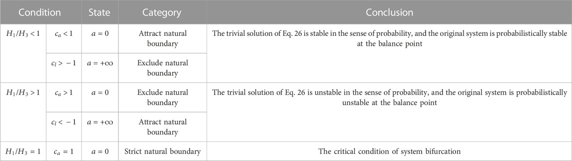
TABLE 1. Global stability analysis.

4.2.2 Stability of nonlinear Itô stochastic differential equation

When ${\alpha }_1,{\alpha }_2,{\alpha }_3,{\alpha }_4,H_2\ne 0$, $a=0$ is the first kind of singular boundary of Eq. 24. When $a=+\infty$ and $m_a=+\infty$, $a=+\infty$ is the second kind of singular boundary problem of Eq. 24. Calculating the diffusion index, drift indices, and characteristic value at boundary $a=0$ and $a=+\infty$, respectively, yields

$\begin{array}{c}{\alpha }_a=2,{\beta }_a=1,\\ c_a=\underset{a\to 0^{+}}{\lim }\frac{2m_a{\left(a-0\right)}^{\left({\alpha }_a-{\beta }_a\right)}}{{{\sigma }_{11}}^2\left(a\right)+{{\sigma }_{12}}^2\left(a\right)}\\ =\underset{a\to 0^{+}}{\lim }\left(\begin{array}{c}-a\left(\epsilon +{\omega }^{p-1}\mathit{sin}\left(\frac{p\pi }{2}\right)\right)+\frac{{\alpha }_1{a}^3}{4}-\frac{{\alpha }_2{a}^5}{8}\\ +\frac{5{\alpha }_3{a}^7}{64}-\frac{7{\alpha }_4{a}^9}{128}+\frac{S_1\left(1\right)}{a{{\omega }_0}^2}+\frac{3a{S}_2\left(1\right)}{4{{\omega }_0}^2}\end{array}\right)a/\left(\frac{S_1\left(1\right)}{{{\omega }_0}^2}+\frac{{a^{2}S}_2\left(1\right)}{4{{\omega }_0}^2}\right)\\ =\underset{a\to 0^{+}}{\lim }\frac{{{\omega }_0}^2\left(\begin{array}{c}-128a^2\left(\epsilon +{\omega }^{p-1}\mathit{sin}\left(\frac{p\pi }{2}\right)\right)+32{\alpha }_1{a}^4-16{\alpha }_2{a}^6\\ +10{\alpha }_3{a}^8-7{\alpha }_4{a}^{10}+128S_1\left(1\right)+96{a^{2}S}_2\left(1\right)\end{array}\right)}{128S_1\left(1\right)+32{a^{2}S}_2\left(1\right)}=1,\lim \\ {\alpha }_l=2,{\beta }_l=9,\\ c_l=-\underset{a\to +\infty }{\lim }\frac{2m_a{\left(a-0\right)}^{\left({\alpha }_l-{\beta }_l\right)}}{{{\sigma }_{11}}^2\left(a\right)+{{\sigma }_{12}}^2\left(a\right)}\\ =-\underset{a\to +\infty }{\lim }\left(\begin{array}{c}-a\left(\epsilon +{\omega }^{p-1}\mathit{sin}\left(\frac{p\pi }{2}\right)\right)+\frac{{\alpha }_1{a}^3}{4}-\frac{{\alpha }_2{a}^5}{8}\\ +\frac{5{\alpha }_3{a}^7}{64}-\frac{7{\alpha }_4{a}^9}{128}+\frac{S_1\left(1\right)}{a{{\omega }_0}^2}+\frac{3a{S}_2\left(1\right)}{4{{\omega }_0}^2}\end{array}\right)a^{-7}/\left(\frac{S_1\left(1\right)}{{{\omega }_0}^2}+\frac{{a^{2}S}_2\left(1\right)}{4{{\omega }_0}^2}\right)\\ =-\underset{a\to +\infty }{\lim }\frac{{{\omega }_0}^2\left(\begin{array}{c}-128a^2\left(\epsilon +{\omega }^{p-1}\mathit{sin}\left(\frac{p\pi }{2}\right)\right)+32{\alpha }_1{a}^4-16{\alpha }_2{a}^6\\ +10{\alpha }_3{a}^8-7{\alpha }_4{a}^{10}+128S_1\left(1\right)+96{a^{2}S}_2\left(1\right)\end{array}\right)}{128S_1\left(1\right)a^8+32S_2\left(1\right)a^{10}}=-\frac{7{\alpha }_4{{\omega }_0}^2}{32S_2\left(1\right)}.\end{array}$

Conclusion: when $a=0$ and $c_a=1$ are a strict natural boundary; when $a=+\infty$ , $c_l>-1$, and $\left({\alpha }_4{{\omega }_0}^2\right)/S_2\left(1\right)<32/7$, the boundary is an exclude natural boundary; when $c_l<-1$ and $\left({\alpha }_4{{\omega }_0}^2\right)/S_2\left(1\right)>32/7$, the boundary is an attract natural boundary; when $c_l=-1$ and $\left({\alpha }_4{{\omega }_0}^2\right)/S_2\left(1\right)=32/7$, the boundary is a strict natural boundary. Therefore, $c_a=1$ is a critical condition of system bifurcation.

5 Stochastic bifurcation analysis

5.1 D-bifurcation

If $H_2=H_3=0$, Eq. 13 becomes a deterministic system without a stochastic bifurcation phenomenon. Therefore, discussing the situation of $H_3\ne 0$ and ${\alpha }_1={\alpha }_2={\alpha }_3={\alpha }_4=H_2=0$, let ${\sigma }_{12}\left(a\right)={\left(H_3/4\right)}^{1/2}a$ and $m\left(a\right)=\left(H_1/8-H_3/8\right)a$, then the continuous dynamic system generated by Eq. 26 is

${\psi }_1\left(t\right)x=x+{\int }_0^{t}m\left({\psi }_1\left(s\right)x\right)ds+{\int }_0^t\sigma \left({\psi }_1\left(s\right)x\right)\circ dB,(27)$

Equation 27 is the only strong solution of Eq. 26 with $x$ as the initial value. When $m\left(0\right)=0$ and ${\sigma }_{12}\left(0\right)=0$, let $m\left(a\right)$ be bounded, for all $a\ne 0$, the elliptic condition ${\sigma }_{12}\left(0\right)\ne 0$ is satisfied, so there is only one stationary probability density. Therefore, the FPK equation corresponding to Eq. 26 is obtained.

$\frac{\partial p}{\partial t}=-\frac{\partial }{\partial a}\left[\left(\frac{H_1}{8}a\right)p\right]-\frac{{\partial }^2}{\partial a^2}\left[\left(\frac{H_3}{4}{a}^2\right)p\right].(28)$

Let $\partial p/\partial t=0$ get the stationary probability density corresponding to Eq. 28

$p\left(a\right)=c\left|{{\sigma }_{12}}^{-1}\left(a\right)\right|\mathit{exp}\left({\int }_0^a\frac{2m\left(u\right)}{{{\sigma }_{12}}^2\left(u\right)}du\right).(29)$

At this time, Eq. 27 has a non-trivial stationary state and a fixed-point equilibrium state. Assuming the invariant measures of these two kinds of stationary states are ${\upsilon }_1$ and ${\vartheta }_1$, respectively, the density is Eq. 29 and ${\vartheta }_1\left(x\right)$, respectively. Hence, the solution of Eq. 28 is

$a\left(t\right)=a\left(0\right)\mathit{exp}\left[{\int }_0^t\left(\dot{m}\left(a\right)+\frac{{\sigma }_{12}\left(a\right){\ddot{\sigma }}_{12}\left(a\right)}{2}\right)ds+{\int }_0^t{\dot{\sigma }}_{12}\left(a\right)d{B}_2\right].(30)$

The Lyapunov exponent of ${\psi }_1$ with respect to estimate $u$ can be defined as follows

${\lambda }_{{\psi }_1}\left(u\right)=\underset{t\to +\infty }{\lim }\frac{1}{t}\mathit{ln}‖a\left(t\right)‖,(31)$

Substituting Eq. 30 into Eq. 31, here ${\sigma }_{12}\left(0\right)=0$ and ${\dot{\sigma }}_{12}\left(0\right)=0$, its Lyapunov exponent of the fixed-point reads

$\begin{array}{c}{\lambda }_{{\psi }_1}\left({\vartheta }_1\right)=\underset{t\to +\infty }{\lim }\frac{1}{t}\left[\mathit{ln}‖a\left(0\right)‖+\dot{m}\left(0\right){\int }_0^{t}ds+{\dot{\sigma }}_{12}\left(0\right){\int }_0^{t}d{B}_2\left(s\right)\right]\\ =\dot{m}\left(0\right)+{\dot{\sigma }}_{12}\left(0\right)\underset{t\to +\infty }{\lim }\frac{B_2\left(t\right)}{t}=\dot{m}\left(0\right)=\frac{H_1}{8}-\frac{H_3}{8}.\end{array}(32)$

Invariant estimate ${\upsilon }_1$ with Eq. 29 as density. Substituting Eq. 30 into Eq. 31. Assuming that $\dot{\sigma }$ and $\dot{m}+\sigma \dot{\sigma }$ are bounded and integrable, respectively, the Lyapunov exponent can be obtained

$\begin{array}{c}{\lambda }_{{\psi }_1}\left({\upsilon }_1\right)=\underset{t\to +\infty }{\lim }\frac{1}{t}{\int }_0^t\left[\dot{m}\left(a\right)+{\sigma }_{12}\left(a\right){\ddot{\sigma }}_{12}\left(a\right)\right]ds={\int }_R\left[\dot{m}\left(a\right)+\frac{{\sigma }_{12}\left(a\right){\ddot{\sigma }}_{12}\left(a\right)}{2}\right]p\left(a\right)da\\ =-2{\int }_R{\left[\frac{m\left(a\right)}{{\sigma }_{12}\left(a\right)}\right]}^{2}p\left(a\right)da\dot{m}\left(0\right)=-2{H_2}^{3/2}\left(\frac{H_1}{8}-\frac{H_3}{8}\right)\mathit{exp}\left(\frac{8}{H_3}\left(\frac{H_1}{8}-\frac{H_3}{8}\right)\right).\end{array}(33)$

Let $\alpha =H_1-H_3$, when $\alpha <0$ and $H_1<H_3$, ${\vartheta }_1$ is stable, ${\upsilon }_1$ is unstable; when $\alpha >0$ and $H_1>H_3$, ${\vartheta }_1$ is unstable, ${\upsilon }_1$ is stable. So $\alpha$ is a D-bifurcation point of Eq. 13.

5.2 P-bifurcation

5.2.1 Stochastic P-bifurcation under additive recycling noise

When additive noise just exists, $D_1\ne 0$ and $D_2=0$. The following is an analysis of the stochastic P-bifurcation of the system in this case. Eq. 22, 23 show that the Itô stochastic differential equation corresponding to $a\left(t\right)$ does not depend upon $\theta \left(t\right)$, and it is a 1-D diffusion process; its corresponding FPK equation can be expressed as

$\frac{\partial p\left(a,t\right)}{\partial t}=-\frac{\partial }{\partial a}\left[m_1\left(a\right)p\left(a,t\right)\right]+\frac{1}{2}\frac{{\partial }^2}{\partial a^2}\left[{{\sigma }_{11}}^2\left(a\right)p\left(a,t\right)\right],(34)$

the corresponding boundary conditions are

$\left\{\begin{array}{c}p=c,c\in \left(-\infty ,+\infty \right),whena=0.\\ p\to 0,\frac{\partial p}{\partial a}\to 0,whena\to \infty .\end{array}\right.(35)$

In view of Eq. 35, the stationary probability density of the amplitude is

$p\left(a\right)=\frac{C}{{{\sigma }_{11}}^2\left(a\right)}\mathit{exp}\left[{\int }_0^a\frac{2m_1\left(u\right)}{{{\sigma }_{11}}^2\left(u\right)}du\right],(36)$

where $C$ is the normalization constant,

$C={\left[{\int }_0^{\infty }\left(\frac{1}{{{\sigma }_{11}}^2\left(a\right)}\mathit{exp}\left[{\int }_0^a\frac{2m_1\left(u\right)}{{{\sigma }_{11}}^2\left(u\right)}du\right]\right)da\right]}^{-1}.(37)$

In view of Eq. 23, from Eq. 36, we obtain

$p\left(a\right)=\frac{Ca{{\omega }_0}^2}{S_1\left(1\right)}\mathit{exp}\left[-\frac{a^2{{\omega }_0}^2\Delta }{7680S_1\left(1\right)}\right],(38)$

where

$\left\{\begin{array}{c}\Delta =3840\epsilon +3840{\omega }^{p-1}\mathit{sin}\left(\frac{p\pi }{2}\right)-480{\alpha }_1{a}^2+160{\alpha }_2{a}^4-75{\alpha }_3+42{\alpha }_4{a}^8,\\ {{\omega }_0}^2={\omega }^2+{\omega }^p\mathit{cos}\left(\frac{p\pi }{2}\right),\\ S_1\left(1\right)=2D_1\left[1+k^2+2kcos\left(\tau \right)\right].\end{array}\right.(39)$

The original system response meets $a\left(t\right)=\sqrt{x^2\left(t\right)+{\dot{x}}^2\left(t\right)}$, in view of Eq. 38, the joint probability density function of the system is

$p\left(a\right)=\frac{C\sqrt{x^2\left(t\right)+{\dot{x}}^2\left(t\right)}{{\omega }_0}^2}{S_1\left(t\right)}\mathit{exp}\left[-\frac{\left(x^2\left(t\right)+{\dot{x}}^2\left(t\right)\right){{\omega }_0}^2}{3840S_1\left(t\right)}\Delta \right].(40)$

5.2.1.1 Influence of fractional order

As fractional damping is a combination of the equivalent stiff and equivalent damping, the fractional order is of paramount importance; its value can be calculated by He-Liu’s fractal formulation [52] for practical applications. According to Eq. 12, when $p=1$, fractional damping becomes a damping term, while when $p=0$, it is a stiff term.

Setting $\tau =2,k=0.4,\epsilon =-0.1,{\alpha }_1=1.51,{\alpha }_2=2.85,{\alpha }_3=1.693,{\alpha }_4=0.312$, and $\omega =1$ in Eq. 13 as that in Refs [30, 53], the stochastic P-bifurcation is studied hereby. Keeping $D_1=0.005$ constant, we draw the joint probability density function section and top view of Eq. 13 under the influence of different fractional orders.

When $p=0.06$, the joint probability density function diagram shows a crater shape; there is only one peak in the section, and there is only a large limit cycle. The response is shown as a vibration far beyond the origin (Figure 1).

FIGURE 1

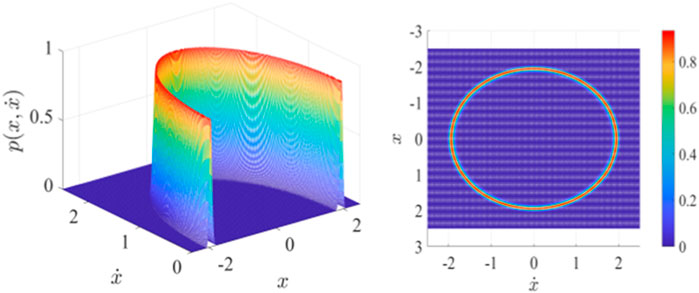
FIGURE 1. Joint probability density function section and top view of Eq. 13 when $\mathbf{p}=\mathbf{0.06}$.

When $p=0.139$, from the section, it can be clearly seen that there are two peaks, but the second peak has a much larger amplitude. At this time, the system has a balance point and a large limit cycle; hence, the system response switches between two peaks, and the probability of a large amplitude vibration is high, as shown in Figure 2.

FIGURE 2

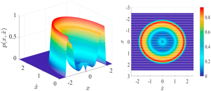
FIGURE 2. Joint probability density function section and top view of Eq. 13 when $\mathbf{p}=\mathbf{0.137}$.

When $p=0.141$, the section has three peaks, showing two peaks in addition to the origin. A balance point now coexists with a large and small limit cycle in the system, and the system response switches between the three peaks, which is a multimodal response. Due to the existence of the double limit point set, the relative heights of the joint probability density function peaks at the three peaks are different, implying that the system response peaks are different, as shown in Figure 3.

FIGURE 3

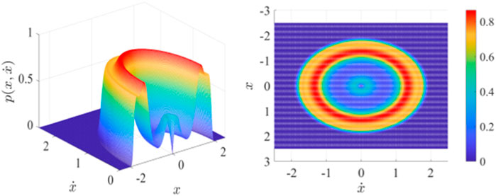
FIGURE 3. Joint probability density function section and top view of Eq. 13 when $\mathbf{p}=\mathbf{0.14}$.

When $p=0.145$, the section has two peaks, in contrast to Figure 2, the relative height of the peak changes, with the second peak being significantly smaller. At this time, the system has both a balance point and a small limit cycle; hence, the system response switches between two peaks, and the probability of a small amplitude vibration is high, as shown in Figure 4.

FIGURE 4

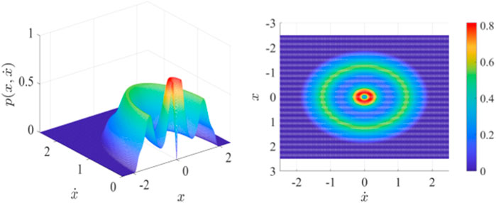
FIGURE 4. Joint probability density function section and top view of Eq. 13 when $\mathbf{p}=\mathbf{0.143}$.

Based on the above discussions, we conclude that the fractional order can cause stochastic P-bifurcation behavior in the system. From Figure 5, we find that an increasing fractional order will change the stationary response from a single mode to a dual mode and then to a tristable mode. The peak value changes from a single peak to two peaks and then to three peaks, so stochastic P-bifurcation occurs. Increasing the value of $p$ to 0.145 again, the tristable disappears and the bistable appears; the peak value changes from three peaks to two peaks, so stochastic P-bifurcation occurs.

FIGURE 5

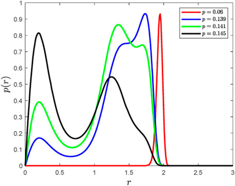
FIGURE 5. Stationary probability density function diagram of Eq. 13 when ${\mathbf{D}}_{\mathbf{1}}=\mathbf{0.005}$.

5.2.1.2 Influence of noise intensity

Keeping the above parameters unchanged, and fixing $p=0.14$, we draw the joint probability density function section and top view of Eq. 13 under the influence of different noise intensity.

When $D_1=0.03$, the joint probability density function diagram shows a crater shape, there is only one peak in the section, and there is only a large limit cycle. The response is shown as a vibration far beyond its origin, as shown in Figure 6.

FIGURE 6

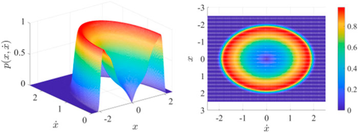
FIGURE 6. Joint probability density function section and top view of Eq. 13 when ${\mathbf{D}}_{\mathbf{1}}=\mathbf{0.03}$.

When $D_1=0.015$, from the section, it can be clearly seen that there are two peaks, but the first peak is much smaller. At this time, the system has both a balance point and a large limit cycle; hence, the system response switches between two peaks, and the probability of a large amplitude vibration is high, as shown in Figure 7.

FIGURE 7

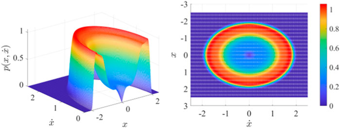
FIGURE 7. Joint probability density function section and top view of Eq. 13 when ${\mathbf{D}}_{\mathbf{1}}=\mathbf{0.015}$.

When $D_1=0.005$, the section has three peaks, showing two peaks in addition to the origin. A balance point now coexists with a large and small limit cycle in the system, and the system response switches among the three peaks, which is a multimodal response. Due to the existence of the double limit point set, the relative heights of the joint probability density function peaks at the three peaks are different, implying that the vibration frequency of the system response peak is different, as shown in Figure 8.

FIGURE 8

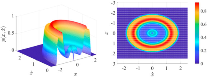
FIGURE 8. Joint probability density function section and top view of Eq. 13 when ${\mathbf{D}}_{\mathbf{1}}=\mathbf{0.005}$.

When $D_1=0.0013$, the section has two peaks, in contrast to Figure 7; the relative height of the peak changes, with the first peak being much larger. At this point, the system has a balance point and a small limit cycle, the system response switches between two peaks, and the probability of a small amplitude vibration is high, as shown in Figure 9.

FIGURE 9

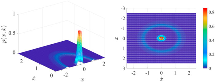
FIGURE 9. Joint probability density function section and top view of Eq. 13 when ${\mathbf{D}}_{\mathbf{1}}=\mathbf{0.0013}$.

Based on the above discussions, it can be verified that changing the noise intensity affects greatly stochastic P-bifurcation property. From Figure 10, it can also be seen that with noise intensity being reduced, the stationary response of the system switches from a single mode to a dual mode and then to a tristable mode. The peak value of the stationary probability density function curve changes from a single peak to two peaks and then three peaks, so stochastic P-bifurcation occurs. Decreasing the value of $D_1$ to 0.0013 again, the tristable disappears and the bistable appears; the peak value changes from three peaks to two peaks, so stochastic P-bifurcation occurs.

FIGURE 10

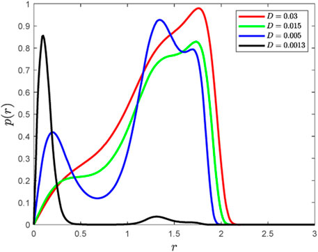
FIGURE 10. Stationary probability density function diagram of Eq. 13 when $\mathbf{p}=\mathbf{0.141}$.

5.2.2 Additive and multiplicative recycling noise

When $D_1\ne 0$ and $D_2\ne 0$, the expression of the stationary probability density function of the amplitude of Eq. 13 is

$p\left(a\right)=\frac{C}{{{\sigma }_{11}}^2\left(a\right)+{{\sigma }_{12}}^2\left(a\right)}\mathit{exp}\left[{\int }_0^a\frac{2m\left(u\right)}{{{\sigma }_{11}}^2\left(u\right)+{{\sigma }_{12}}^2\left(u\right)}du\right],(41)$

where $C$ is the normalization constant,

$C={\left[{\int }_0^{\infty }\left(\frac{1}{{{\sigma }_{11}}^2\left(a\right)+{{\sigma }_{12}}^2\left(a\right)}\mathit{exp}\left[{\int }_0^a\frac{2m_1\left(u\right)}{{{\sigma }_{11}}^2\left(u\right)+{{\sigma }_{12}}^2\left(u\right)}du\right]\right)da\right]}^{-1}.(42)$

In view of Eq. 23, from Eq. 42, we have

$p\left(a\right)=4Ca{{\omega }_0}^2{\left[4S_1\left(1\right)+a^2{S}_2\left(1\right)\right]}^{-\frac{{\Delta }_1}{{S_2}^5\left(1\right)}}\mathit{exp}\left(\frac{{\Delta }_2}{768{S_2}^4\left(1\right)}\right),(43)$

where

$\left\{\begin{array}{c}{\Delta }_1=2{{\omega }_0}^2\left[\left(\epsilon +{\omega }^{p-1}\mathit{sin}\left(\frac{p\pi }{2}\right)\right){S_2}^4+{\alpha }_1{S}_1{S_2}^3+2{\alpha }_2{S_1}^2{S_2}^2+5{\alpha }_3{S_1}^3{S}_2+14{\alpha }_4{S_1}^4\right],\\ {\Delta }_1=a^2{{\omega }_0}^2\left(384{\alpha }_1{S_2}^3+768{\alpha }_2{S}_1{S_2}^2+1920{\alpha }_3{S_1}^2{S}_2+5376{\alpha }_4{S_1}^3\right)\\ +a^4{{\omega }_0}^2\left(-96{\alpha }_2{S_2}^3-240{\alpha }_3{S}_1{S_2}^2-672{\alpha }_4{S_1}^2{S}_2\right)\\ +a^6{{\omega }_0}^2\left(40{\alpha }_3{S_2}^3+112{\alpha }_4{S}_1{S_2}^2\right)-21a^8{{\omega }_0}^2{\alpha }_4{S_2}^3,\\ {{\omega }_0}^2={\omega }^2+{\omega }^p\mathit{cos}\left(\frac{p\pi }{2}\right),\\ S_1\left(1\right)=2D_1\left[1+k^2+2kcos\left(\tau \right)\right],S_2\left(1\right)=2D_2\left[1+k^2+2kcos\left(\tau \right)\right].\end{array}\right.(44)$

Keeping the above parameters unchanged, we draw the joint probability density function section and top view of Eq. 13 under the influence of different fractional orders and noise intensity.

When $p=0.05$, let $D_1=0.5$ and $D_2=1$. The joint probability density function diagram shows a crater shape; there is only one peak in the section, and there is only a large limit cycle. The response is shown as a vibration far away from the origin. At the same time, reducing the value of noise intensity reveals that the peak of the joint probability density does not change with only one peak. However, the system only has a limit cycle, which has been in a monostable. Therefore, there is no stochastic P-bifurcation phenomenon occurring, as shown in Figure 11.

FIGURE 11

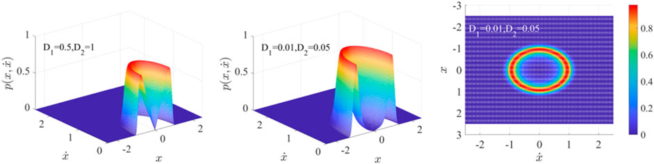
FIGURE 11. Joint probability density function section and top view of Eq. 13 when $\mathbf{p}=\mathbf{0.05}$.

When $p=0.1$, let $D_1=0.002$ and $D_2=0.01$. From the section, it can be clearly seen that there are two peaks, but the second peak has a much larger amplitude. At this time, the system has both a balance point and a limit cycle; hence, the system response switches between two peaks, and the large amplitude vibration has a higher probability. When the simultaneous improvement of the noise intensifies to $D_1=0.008$ and $D_2=0.2$, the peak value of the stationary probability density function curve changes from two peaks to one peak. There is only a large limit cycle, and the system response becomes a vibration far from the origin. Therefore, increasing the noise intensity induces a stochastic P-bifurcation property, as shown in Figure 12.

FIGURE 12

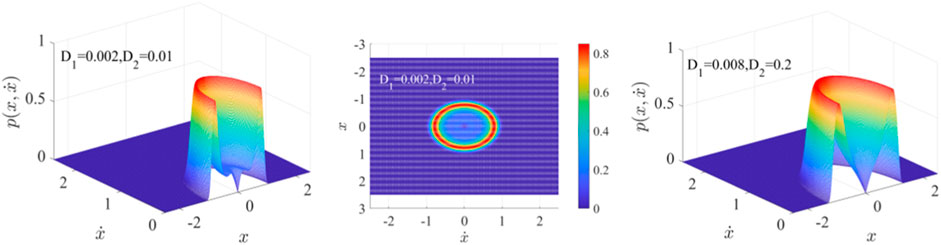
FIGURE 12. Joint probability density function section and top view of Eq. 13 when $\mathbf{p}=\mathbf{0.1}$.

When $p=0.14$, let $D_1=0.003$ and $D_2=0.01$. The section has a peak near the origin. There is only a balance point in the system at this time, and the response is shown as a vibration closer to the origin. When simultaneously improving its noise intensity to $D_1=0.004$ and $D_2=0.1$, the peak value of the stationary probability density function curve changes from a single peak to two peaks. At this time, the system has both a balance point and a limit cycle; hence, the system response switches between two peaks, and the probability of a large amplitude vibration is small. Therefore, increasing the noise intensity induces the stochastic P-bifurcation phenomenon. Further increasing the noise intensity to $D_1=0.006$ and $D_2=0.15$, the peak value of the section changes relatively, and the first peak is lower. The system response switches between two peaks, and the probability of a small one is small. Continuing to increase the value of noise intensity to $D_1=0.04$ and $D_2=0.3$, the peak value of the curve changes from two peaks to a single peak. There is only a limit cycle in the system at this time, and the response is shown as a vibration far away from the origin. Therefore, increasing the noise intensity induces the second stochastic P-bifurcation phenomenon, as show in Figure 13.

FIGURE 13

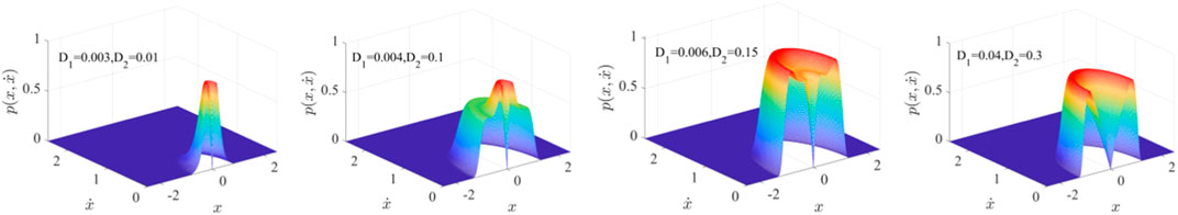
FIGURE 13. Joint probability density function section and top view of Eq. 13 when $\mathbf{p}=\mathbf{0.14}$.

6 Conclusion

In this paper, the stationary response and the stochastic bifurcation of the fractional van der Pol equation under multiplicative and additive recycling noise excitations are investigated. By the least square method, we obtain an equivalent integral nonlinear stochastic system. The Itô differential equation and One-dimensional Markov process are obtained according to the stochastic averaging method. We discuss the local and global stochastic stability and analyze the conditions for inducing D-bifurcation and P-bifurcation in the system. The analysis shows that when $\alpha <0$ and $H_1<H_3$, the point equilibrium state becomes stable, and the non-trivial stationary state becomes unstable; when $\alpha >0$ and $H_1>H_3$, the result is the opposite. So $\alpha$ is a D-bifurcation point of the original system. When only additive noise exists, the fractional order and the noise intensity will greatly affect the system’s property. It was found that reducing the order $p$ or increasing the noise intensity $D_1$ can cause nonlinear jumping or significant oscillation in the system, leading to system instability. Through increasing the order $p$ or reducing the noise intensity $D_1$, the system response is in a monostable state or a small disturbance near the balance point. Similarly, when additive and multiplicative noise coexist, selecting appropriate parameters can maintain the system response at a monostable or small disturbance near the balance point. Therefore, in practical engineering, to avoid the potential adverse effects of high noise intensity on the system, the occurrence of stochastic bifurcation behavior can be controlled by changing the noise intensity or fractional order. In the future, we will combine theory with practice to explore the impact of recycling noise on the stationary response and stochastic bifurcation of systems in wind turbines. We will study the impact of changing noise intensity and fractional order on the system, and how to handle these adverse effects to achieve optimal system performance.

Data availability statement

The original contributions presented in the study are included in the article/Supplementary material, further inquiries can be directed to the corresponding author.

Author contributions

J-GZ: supervision, writing–review and editing, funding acquisition, investigation, and project administration. FW: writing–original draft, writing–review and editing, and software. H-NW: writing–review and editing and software. All authors contributed to the article and approved the submitted version.

Funding

This study was supported by the key project of the Gansu Province natural science foundation of China (No. 23JRRA882).

Conflict of interest

The authors declare that the research was conducted in the absence of any commercial or financial relationships that could be construed as a potential conflict of interest.

Publisher’s note

All claims expressed in this article are solely those of the authors and do not necessarily represent those of their affiliated organizations, or those of the publisher, the editors and the reviewers. Any product that may be evaluated in this article, or claim that may be made by its manufacturer, is not guaranteed or endorsed by the publisher.

References

1. He JH. A tutorial review on fractal spacetime and fractional calculus. Int J Theor Phys (2014) 53:3698–718. doi:10.1007/s10773-014-2123-8

CrossRef Full Text | Google Scholar

2. He JH. Fractal calculus and its geometrical explanation. Phys (2018) 10:272–6. doi:10.1016/j.rinp.2018.06.011

CrossRef Full Text | Google Scholar

3. He CH, Liu C. Fractal approach to the fluidity of a cement mortar. Nonlinear Engineering-modeling Appl (2022) 11(1):1–5. doi:10.1515/nleng-2022-0001

CrossRef Full Text | Google Scholar

4. Zuo YT, Liu HJ. Fractal approach to mechanical and electrical properties of graphene/sic composites. Facta Universitatis: Ser Mech Eng (2021) 19(2):271–84. doi:10.22190/fume201212003z

CrossRef Full Text | Google Scholar

5. He CH, Liu C. Fractal dimensions of a porous concrete and its effect on the concrete’s strength. Facta Universitatis Ser Mech Eng (2023) 21(1):137–50. doi:10.22190/FUME221215005H

CrossRef Full Text | Google Scholar

6. Jankowski P. Detection of nonlocal calibration parameters and range interaction for dynamic of FGM porous nanobeams under electro-mechanical loads. Facta Universitatis Ser Mech Eng (2022) 20(3):457–78. doi:10.22190/fume210207007j

CrossRef Full Text | Google Scholar

7. He CH, Shen Y, Ji FY, He JH. Taylor series solution for fractal Bratu-type equation arising in electrospinning process. Fractals (2020) 28(1):2050011. doi:10.1142/s0218348x20500115

CrossRef Full Text | Google Scholar

8. Liu FJ, Zhang T, He CH, Tian D. Thermal oscillation arising in a heat shock of a porous hierarchy and its application. Facta Universitatis Ser Mech Eng (2022) 20(3):633–45. doi:10.22190/fume210317054l

CrossRef Full Text | Google Scholar

9. Liang YH, Wang KJ. A new fractal viscoelastic element: Promise and applications to Maxwell-Rheological model. Therm Sci (2021) 25(2):1221–7. doi:10.2298/tsci200301015l

CrossRef Full Text | Google Scholar

10. Zuo YT. Effect of Sic particles on viscosity of 3-D print paste a fractal rheological model and experimental verification. Therm Sci (2021) 25(3):2405–9. doi:10.2298/tsci200710131z

CrossRef Full Text | Google Scholar

11. Long Y, Xu BB, Chen DY, Ye W. Dynamic characteristics for a hydro-turbine governing system with viscoelastic materials described by fractional calculus. Appl Math Model (2018) 58:128–39. doi:10.1016/j.apm.2017.09.052

CrossRef Full Text | Google Scholar

12. Wang L, Xue LL, Xu W, Yue XL. Stochastic P-bifurcation analysis of a fractional smooth and discontinuous oscillator via the generalized cell mapping method. Int J Non-Linear Mech (2017) 96:56–63. doi:10.1016/j.ijnonlinmec.2017.08.003

CrossRef Full Text | Google Scholar

13. He CH, Amer TS, Tian D, Abolila AF, Galal AA. Controlling the kinematics of a spring-pendulum system using an energy harvesting device. J Low Frequency Noise: Vibration Active Control (2022) 41(3):1234–57. doi:10.1177/14613484221077474

CrossRef Full Text | Google Scholar

14. He CH, Ei-Dib YO. A heuristic review on the homotopy perturbation method for non-conservative oscillators. J Low FrequCency Noise, Vibration Active Control (2022) 41(2):572–603. doi:10.1177/14613484211059264

CrossRef Full Text | Google Scholar

15. He JH, Ei-Dib YO. The reducing rank method to solve third-order Duffing equation with the homotopy perturbation. Numer Methods Differential Equations (2021) 37(2):1800–8. doi:10.1002/num.22609

CrossRef Full Text | Google Scholar

16. Zhang WT, Xu W, Niu LZ, Tang YN. Bifurcations analysis of a multiple attractors energy harvesting system with fractional derivative damping under random excitation. Commun Nonlinear Sci Numer Simulation (2023) 118:107069. doi:10.1016/j.cnsns.2022.107069

CrossRef Full Text | Google Scholar

17. Hu DL, Mao XC, Han L. Stochastic stability analysis of a fractional viscoelastic plate excited by Gaussian white noise. Mech Syst Signal Process (2022) 177:109181. doi:10.1016/j.ymssp.2022.109181

CrossRef Full Text | Google Scholar

18. Li YJ, Wu ZQ, Lan QX, Cai YJ, Xu HF, Sun YT. Stochastic transition behaviors in a Tri-Stable van der Pol oscillator with fractional delayed element subject to Gaussian White Noise. Therm Sci (2022) 26(3):2713–25. doi:10.2298/tsci2203713l

CrossRef Full Text | Google Scholar

19. Li YJ, Wu ZQ, Lan QX, Cai YJ, Xu HF, Sun YT. Transition behaviors of system energy in a bi-stable van Ver Pol oscillator with fractional derivative element driven by multiplicative Gaussian white noise. Therm Sci (2022) 26(3):2727–36. doi:10.2298/tsci2203727l

CrossRef Full Text | Google Scholar

20. Li YJ, Wu ZQ, Wang F, Zhang GQ, Wang YC. Stochastic P-bifurcation in a generalized Van der Pol oscillator with fractional delayed feedback excited by combined Gaussian white noise excitations. J Low Frequency Noise, Vibration Active Control (2021) 40(1):91–103. doi:10.1177/1461348419878534

CrossRef Full Text | Google Scholar

21. Din A, Ain QT. Stochastic optimal control analysis of a mathematical model: Theory and application to non-singular kernels. fractal and fractional (2022) 6:279. doi:10.3390/fractalfract6050279

CrossRef Full Text | Google Scholar

22. Zhu R, Wang MX, Xu SY, Li K, Han QP, Tong X, et al. Fault diagnosis of rolling bearing based on singular spectrum analysis and wide convolution kernel neural network. J Low Frequency Noise, Vibration Active Control (2022) 41(4):1307–21. doi:10.1177/14613484221104639

CrossRef Full Text | Google Scholar

23. Kuo PH, Tseng YR, Luan PC, Yau HT. Novel fractional-order convolutional neural network based chatter diagnosis approach in turning process with chaos error mapping. Nonlinear Dyn (2023) 111:7547–64. doi:10.1007/s11071-023-08252-w

CrossRef Full Text | Google Scholar

24. Kuo PH, Chen YW, Hsieh TH, Jywe WY, Yau HT. A thermal displacement prediction system with an automatic Lrgtvac-PSO optimized branch Structured bidirectional GRU neural network. IEEE Sensors Journa (2023) 23:12574–86. doi:10.1109/JSEN.2023.3269064

CrossRef Full Text | Google Scholar

25. He JH, Jiao ML, Gepreel KA, Khan Y. Homotopy perturbation method for strongly nonlinear oscillators. Mathematics Comput Simulation (2023) 204:243–58. doi:10.1016/j.matcom.2022.08.005

CrossRef Full Text | Google Scholar

26. He JH, Jiao ML, He CH. Homotopy perturbation method for fractal Duffing oscillator with arbitrary conditions. Fractals (2022) 30. doi:10.1142/S0218348X22501651

CrossRef Full Text | Google Scholar

27. Chen LC, Zhu WQ. Stochastic jump and bifurcation of Duffing oscillator with fractional derivative damping under combined harmonic and white noise excitations. Int J Non-Linear Mech (2011) 46:1324–9. doi:10.1016/j.ijnonlinmec.2011.07.002

CrossRef Full Text | Google Scholar

28. Chen LC, Zhu WQ. Stationary response of duffing oscillator with fractional derivative damping under combined harmonic and wide band noise excitations. Chin J Appl Mech (2010) 3:517–21.

Google Scholar

29. He CH, Tian D, Moatimid GM, Salman HF, Zekry MH. Hybrid Rayleigh–van der pol–duffing oscillator: Stability analysis and controller. J Low Frequency Noise, Vibration Active Control (2022) 41(1):244–68. doi:10.1177/14613484211026407

CrossRef Full Text | Google Scholar

30. Li YJ, Wu ZQ. Stochastic P-bifurcation in a tri-stable Van der Pol system with fractional derivative under Gaussian white noise. J Vibroengineering (2019) 21:803–15. doi:10.21595/jve.2019.20118

CrossRef Full Text | Google Scholar

31. Li YJ, Wu ZQ, Lan QX, Hao Y, Zhang XY. Stochastic P bifurcation in a tri-stable van der Pol oscillator with fractional derivative excited by combined Gaussian white noises. J Vibration Shock (2021) 40(16):275–93. doi:10.21595/jve.2019.20118

CrossRef Full Text | Google Scholar

32. Chamgoué AC, Yamapi R, Woafo P. Bifurcations in a biorhythmic biological system with time-delayed noise. Nonlinear Dyn (2013) 73:2157–73. doi:10.1007/s11071-013-0931-7

CrossRef Full Text | Google Scholar

33. Wu YZ, Sun ZK. Residence-times distribution function in asymmetric bistable system driven by noise recycling. Acta Phys Sin (2020) 69(12):120501. doi:10.7498/aps.69.20201752

CrossRef Full Text | Google Scholar

34. Guo XY, Cao TQ. Phenomenon of double entropic stochastic resonance with recycled noise. Chin J Phys (2022) 77:721–32. doi:10.1016/j.cjph.2021.10.020

CrossRef Full Text | Google Scholar

35. He KY, Nadeem M, Habib S, Sedighi HM, Huang DH. Analytical approach for the temperature distribution in the casting-mould heterogeneous system. Int J Numer Methods Heat Fluid Flow (2021) 32:1168–82. doi:10.1108/HFF-03-2021-0180

CrossRef Full Text | Google Scholar

36. Fang JH, Nadeem M, Habib M, Karim S, Wahash HA. A new iterative method for the approximate solution of klein-gordon and sine-gordon equations. J Funct Spaces (2022) 2022:1–9. doi:10.1155/2022/5365810

CrossRef Full Text | Google Scholar

37. He JH, Kou SJ, He CH, Zhang ZW, Gepreel KA. Fractal oscillation and its frequency-amplitude property. Fractals (2021) 29(4):2150105. doi:10.1142/s0218348x2150105x

CrossRef Full Text | Google Scholar

38. He JH, Moatimid G, Zekry M. Forced nonlinear oscillator in a fractal space. Facta Universitatis, Ser Mech Eng (2022) 20(1):001–20. doi:10.22190/fume220118004h

CrossRef Full Text | Google Scholar

39. Tian D, Ain QT, Anjum N, He CH, Cheng B. Fractal N/MEMS: From pull-in instability to pull-in stability. Fractals (2021) 29:2150030. doi:10.1142/S0218348X21500304

CrossRef Full Text | Google Scholar

40. He CH. A variational principle for a fractal nano/microelectromechanical (N/MEMS) system. Intermational J Numer Methods Heat Fluid Flow (2023) 33(1):351–9. doi:10.1108/hff-03-2022-0191

CrossRef Full Text | Google Scholar

41. Ain QT, Sathiyaraj Karim S, Nadeem M, Mwanakatwe PK, Kandege Mwanakatwe P. ABC fractional derivative for the alcohol drinking model using two-scale fractal dimension. Complexity (2022) 2022:1–11. doi:10.1155/2022/8531858

CrossRef Full Text | Google Scholar

42. Wang Y, An JY. Amplitude-frequency relationship to a fractional Duffing oscillator arising in microphysics and tsunami motion. J Low Frequency Noise Vibration Active Control (2019) 38(3-4):1008–12. doi:10.1177/1461348418795813

CrossRef Full Text | Google Scholar

43. Mendes EM, Salgado GH, Aguirre LA. Numerical solution of Caputo fractional differential equations with infinity memory effect at initial condition. Commun Nonlinear Sci Numer Simulation (2019) 69:237–47. doi:10.1016/j.cnsns.2018.09.022

CrossRef Full Text | Google Scholar

44. Zeng HJ, Wang YX, Xiao M, Wang Y. Fractional solitons: New phenomena and exact solutions. Front Phys (2023) 11:1177335. doi:10.3389/fphy.2023.1177335

CrossRef Full Text | Google Scholar

45. Chen LC, Wang WH, Li ZS, Zhu WQ. Stationary response of Duffing oscillator with hardening stiffness and fractional derivative. Int J Non-Linear Mech (2013) 48:44–50. doi:10.1016/j.ijnonlinmec.2012.08.001

CrossRef Full Text | Google Scholar

46. Li W, Zhang MT, Zhao JF. Stochastic bifurcations of generalized Duffing-van der Pol system with fractional derivative under colored noise. Chin Phys B (2017) 26:090501. doi:10.1088/1674-1056/26/9/090501

CrossRef Full Text | Google Scholar

47. Chen LC, Li ZS, Zhuang QQ, Zhu WQ. First-passage failure of single-degree-of-freedom nonlinear oscillators with fractional derivative. J Vibration Control (2013) 19:2154–63. doi:10.1177/1077546312456057

CrossRef Full Text | Google Scholar

48. Chen LC, Zhu WQ. Stochastic response of fractional-order van der Pol oscillator. Theor Appl Mech Lett (2014) 4:013010. doi:10.1063/2.1401310

CrossRef Full Text | Google Scholar

49. Spanos PD, Zeldin BA. Random vibration of systems with frequency-dependent parameters or fractional derivatives. J Eng Mech (1997) 123(3):290–2. doi:10.1061/(asce)0733-9399(1997)123:3(290)

CrossRef Full Text | Google Scholar

50. Zhu WQ. Nonlinear stochastic dynamics and control: Hamilton theoretical framework. Beijing, China: Science Press (2003).

Google Scholar

51. Oseledec VI. A multiplicative ergodic theorem. Lyapunov characteristic numbers for dynamical systems. Trans Mosc Math. Soc (1968) 19(2):197–231.

Google Scholar

52. He CH, Liu C. Fractal dimensions of a porous concrete and its effect on the concrete’s strength. Facta Universitatis Ser Mech Eng (2023) 21(1):137–50. doi:10.22190/FUME221215005H

CrossRef Full Text | Google Scholar

53. Zhang XY, Wu ZQ. Bifurcations in tri-stable Duffing–Van der Pol oscillator with recycling noise. Mod Phys Lett B (2018) 32(20):1850228. doi:10.1142/s0217984918502287

CrossRef Full Text | Google Scholar