Complex solutions for nonlinear fractional partial differential equations via the fractional conformable residual power series technique and modified auxiliary equation method

The fractional-order nonlinear Gardner and Cahn–Hilliard equations are often used to model ultra-short burst beams of light, complex fields of optics, photonic transmission systems, ions, and other fields of mathematical physics and engineering. This study has two main objectives. First, the main objective of this investigation is to solve the fractional-order nonlinear Gardner and Cahn–Hilliard equations by using the modified auxiliary equation method, which is not found in the literature. Second, the exact and approximate solutions of these equations are obtained by utilizing the fractional conformable residual power series algorithm and the modified auxiliary equation method. For the analytical and numerical solutions to two equations, we employ two separate techniques and establish consistency between the precise answers that are derived and the compatible numerical solution. To the best of our knowledge, this method of solving equations has never been investigated in this manner. The 2D and 3D contours have been defined using appropriate parametric values to support the physical compatibility of the results. The assessed findings suggested that the approach used in this study to recover inclusive and standard solutions is approachable, efficient, and faster in computing and can be considered a useful tool in resolving more complex phenomena that arise in the field of engineering, mathematical physics, and optical fiber.

1 Introduction

In complicated areas of fields that can be modeled by various types of partial differential equations, many linear and nonlinear solutions appear. The nonlinear partial differential equations (NLPDEs) are crucial for studying a variety of issues. Understanding virtually nonlinear partial differential equations requires an effort to determine precise solutions to nonlinear equations [1–3]. Fractional calculus, which is the study of integrals and derivatives of any arbitrary real or complex order, has gained significant recognition over the past 30 years or so largely because of its well-established applications in numerous and varied disciplines of technical knowledge [4].

Fractional differential equations have received considerable attention over the past 20 years as a result of their capacity to accurately reproduce a broad range of events in a variety of scientific and technical fields. In science and engineering, fractional differential equations can be used to represent a variety of physical applications [5]. Fractional differential equations have been used to tackle numerous engineering and scientific problems [6]. The differential equation in fractional nonlinear partial differential equations (FNLPDEs) has nonlinear variables which create complex behaviors and phenomena not seen in linear equations. Complex patterns, chaotic dynamics, solitons, and shocks can all occur as a result of nonlinearity. The interaction between nonlinearity and fractional derivatives makes it particularly difficult to comprehend and analyze the dynamics of FNLPDEs.

The usage of fractional differential equations (FDEs) is widespread throughout many scientific disciplines due to their various applications in physics and engineering. Fractional partial differential equations (FPDEs) have grown in significance and reputation among FDEs in recent years as a result of their demonstrated utility in a wide range of extremely diverse scientific and engineering disciplines [7]. Many fractional types of equations are solved using novel transform [8] and zz transform with the Mittag-Leffler kernel [9]. Since they cannot be solved precisely, the majority of nonlinear FDEs require approximate and numerical solutions such as the Adomian decomposition method [10], spectral collocation method [11], Euler method and homotopy analysis method [12], Laplace residual power series [13], variational iteration transform method [14], and homotopy analysis method [15]. FNLPDEs find applications in various cutting-edge areas of research. For example, in materials science, FNLPDEs are used to model diffusion and transport in heterogeneous media. In finance, they are employed to describe complex price dynamics and risk management. In biology, FNLPDEs are utilized to study the spread of diseases and population dynamics. The unique combination of nonlinearity and fractional derivatives in FNLPDEs provides a versatile framework for modeling these emerging phenomena.

One of the most recent methods developed in this field is the auxiliary equation method proposed by Khater [16]. Although this approach was employed in numerous research studies [17], a modified auxiliary equation approach (also known as the modified Khater method) was developed to get precise traveling wave solutions. The soliton and other solitary wave solutions of the equations are obtained in this research paper using the modified auxiliary equation approach. It enhances the auxiliary equation method. This article describes a method that modifies the auxiliary differential equation methodology for solving nonlinear partial differential equations [18]. Over the past 30 years, fresh and state-of-the-art methods for investigating nonlinear differential systems with fractional-order equations have been created, along with new computer methods and symbolic programming. Analytical methodologies, new mathematical theories, and computational systems that enable us to study nonlinear complicated phenomena have triggered this revolution in understanding. Furthermore, the sub-equation method [19], modified Kudryashov method [20], and F-expansion method [21–23] are just a few of the methods that have been used.

A semi-approximate approach called numerical simulations was developed specifically for addressing challenging nonlinear temporal FPDEs that can appear in a variety of scientific fields. This approach, which was devised and developed by Abu Arqub for the study of fuzzy differential equations, is used for generalizing the expansion of the Taylor series of arbitrary order and minimizing the residual error identified to detect the unknown compounds. This method has the ability to immediately solve nonlinear terms without any constraints, transformations, linearizations, or changes to the models. As a result, it has attracted considerable attention and has become an energizing focus of the research community [24, 25].

The Gardner equation [26] is developed to illustrate the description of solitary inner waves in shallow water and combines the KdV and modified KdV equations. The Gardner equation is frequently used in various branches of physics, such as plasma theories, quantum area theories, fluid mechanics, and physics [27]. Numerous wave phenomena in the plasma and solid phases are also covered [28]. We recognize the conformable fractional-order nonlinear Gardner (FG) equation in the following form:

${\partial }_t^{\alpha }w\left(x,t\right)+6\left(w-{\lambda }^2{w}^2\right)\frac{\partial w}{\partial x}-\frac{{\partial }^{3}w}{\partial x^3}=0,(1)$

with an initial condition

$w\left(x,0\right)=\frac{1}{2}+\frac{1}{2}\tanh \left(\frac{x}{2}\right),$

and boundary condition

$w\left(0,t\right)=\frac{1}{2}+\frac{1}{2}\tanh \left(\frac{-t}{2}\right),$

$w\left(1,t\right)=\frac{1}{2}+\frac{1}{2}\tanh \left(\frac{1-t}{2}\right).$

A binary alloy’s phase separation under a critical temperature is illustrated by the Cahn–Hilliard equation, which was first proposed by Cahn and Hilliard in 1958 [29]. The spinodal decomposition, phase separation, and phase ordering dynamics are three fascinating physical phenomena that depend critically on this equation [30]. In this framework, the fractional Cahn–Hilliard (FCH) equation [31] is expressed as follows:

${\partial }_t^{\alpha }w\left(x,t\right)-\frac{\partial w}{\partial x}-6w{\left(\frac{\partial w}{\partial x}\right)}^2-\left(3w^2-1\right)\frac{{\partial }^{2}w}{\partial x^2}+\frac{{\partial }^{4}w}{\partial x^4}=0,(2)$

with an initial condition

$w\left(x,0\right)=\tanh \left(\frac{\sqrt{2}\left(x\right)}{2}\right),$

and boundary condition

$w\left(0,t\right)=\tanh \left(\frac{\sqrt{2}\left(t\right)}{2}\right),$

$w\left(1,t\right)=\tanh \left(\frac{\sqrt{2}\left(1+t\right)}{2}\right).$

The methodology of this paper includes the following: Section 2 discusses the modified auxiliary equation method (MAEM) and also solves the equations. Section 3 discusses the semi-analytical fractional conformable residual power series algorithm and contains an explanation of the system to a solution. Section 4 examines the stability property of the equations. Section 5 contains the discussion and results of the system to illustrate the approximate delicacy. Section 6 presents the conclusion.

Preliminaries

Definition 1. The α-order fractional conformable derivative of a function w(x, t) of order αϵ(0, 1) is given as

$\frac{{\partial }^{\alpha }w\left(t\right)}{\partial t}=\underset{ϵ\to 0}{\lim }\frac{w\left(ϵt^{1-\alpha }+t\right)-w\left(t\right)}{ϵ},t>0.$

Moreover, if the previous limit exists at a point s; s > 0 in (0, s), then w(t) is called α-differentiable so that $\frac{{\partial }^{\alpha }w(s)}{\partial t}={\lim }_{t\to s^{+}}\frac{{\partial }^{\alpha }w(t)}{\partial t}$.

Definition 2. The multiple time-fractional series (MTFS) expansion t₀ > 0 is given as

$\sum _{i=0}^{\infty }{\zeta }_i\left(x\right){\left(t-t_0\right)}^{\text{i}\alpha }={\zeta }_0\left(x\right)+{\zeta }_1\left(x\right){\left(t-t_0\right)}^{\alpha }+\dots ,$

where ϵ(n − 1, n), tϵ(t₀, t₀ + r^1/α), r > 0, r^1/α is a radius of convergence and ζ_i(x) indicates unknown coefficients of the expansion. When α = 1, then the expansion in Definition 2 reduces to the usual series expansion at t₀ > 0, with a radius of convergence r that converges uniformly on |t − t₀| < r. Many other definitions are provided in [32].

2 Methodology

2.1 Modified auxiliary equation method

First, we introduce the MAEM [33]. Let us consider FNLPDEs.

$F\left(v,v_t^{\alpha },v_{xx},,v_{xt},,\dots \right)=0,(3)$

where F is the function’s polynomial. In Eq. 3, v is a function of the spatial variables x and t and represents the propagation of the wave profile. To modify the following, Eq. 3 is transformed into an ordinary differential equation as

$v=V\left(\eta \right),\eta =x-\frac{v{t}^{\alpha }}{\alpha },(4)$

where α represents arbitrary constants. Eq. 3 is converted into an ODE of the kind using transforms from Eq. 4.

$M\left(V,V^{\prime },V^{″},\dots \right)=0,(5)$

where M stands for the polynomial involving the function V and its regular derivatives V′ = dV/dη. The solution to Eq. 5 is

$V\left(\eta \right)=a_0+\sum _{i=1}^m\left(a_i{L}^{i\varphi \left(\eta \right)}+a_{-i}{\left(L\right)}^{-i\varphi \left(\eta \right)}\right),(6)$

where a₀ and a_i are unknown constants. Function ϕ′(η) is expressed as

${\varphi }^{\prime }\left(\eta \right)=\frac{\theta L^{\varphi \left(\eta \right)}+\vartheta L^{-\varphi \left(\eta \right)}+\sigma }{\text{In}\left(L\right)},(7)$

where σ, θ, and ϑ are arbitrary constants and L ≠ 1, L > 0. On the basis of the (HBP), we may calculate N. The formal solution to Eq. 5 is obtained by replacing the N in Eq. 6. By substituting the ODE Eq. 7 formal solution into Eq. 5 and setting the coefficients of L^iϕ(η), i = 0, ±1, ±2 … to zero, the system of linear equations is produced. The unknown constants a₀, a_i, and a_−i can be found by solving this system of equations. The following solutions for auxiliary Eq. 7 are taken into consideration as follows:

Case I. When ϑ ≠ 0, σ² − 4θϑ < 0,

$L^{\varphi \left(\eta \right)}=\frac{-\sigma +\sqrt{-{\sigma }^2+4\theta \vartheta }\tan \left(\frac{1}{2}\sqrt{-{\sigma }^2+4\theta \vartheta }\eta \right)}{2\vartheta },(8)$

or

$L^{\varphi \left(\eta \right)}=-\frac{\sigma +\sqrt{-{\sigma }^2+4\theta \vartheta }\cot \left(\frac{1}{2}\sqrt{-{\sigma }^2+4\theta \vartheta }\eta \right)}{2\vartheta }.(9)$

Case II. When ϑ ≠ 0, σ² − 4θϑ > 0,

$L^{\varphi \left(\eta \right)}=-\frac{\sigma +\sqrt{-{\sigma }^2+4\theta \vartheta }\tanh \left(\frac{1}{2}\sqrt{-{\sigma }^2+4\theta \vartheta }\eta \right)}{2\vartheta },(10)$

or

$L^{\varphi \left(\eta \right)}=-\frac{\sigma +\sqrt{-{\sigma }^2+4\theta \vartheta }\coth \left(\frac{1}{2}\sqrt{-{\sigma }^2+4\theta \vartheta }\eta \right)}{2\vartheta }.(11)$

Case III. When ϑ ≠ 0, σ² − 4θϑ = 0,

$L^{\varphi \left(\eta \right)}=-\frac{\sigma \eta +2}{2\vartheta \eta }.(12)$

By substituting the unknown values for a₀, a_i, a₋i and the aforementioned cases into Eq. 6, using transformations from Eq. 4, it is possible to obtain the closed-form solutions to Eq. 1 and Eq. 2.

2.1.1 Application to the fractional-order nonlinear Gardner equation

The governing Eq. 1 transforms into the following ODE using the following conformable derivative transformation from Eq. 4:

$-v{V}^{\prime }+V^{\left(3\right)}+6\left(V-{\lambda }^2{V}^2\right)V^{\prime }=0,$

$-vV+V^{″}-2{\lambda }^2{V}^3+3V^2=0.(13)$

By changing the degree of the highest-order derivative term and nonlinear with HBP, N = 1 is calculated. According to the formal solution in Eq. 13 derived from Eq. 6, we obtain

$V\left(\eta \right)=a_0+a_1{L}^{\varphi \left(\eta \right)}+\frac{a_{-1}}{L^{\varphi \left(\eta \right)}}.(14)$

When Eq. 14 is substituted with Eq. 7 in Eq. 13, the coefficients of powers of L^iϕ(η), i = 0, ±1, ±2 … are set to zero, resulting in a linear equation system. The following sets of solutions are found by using Mathematica software.

Set 1:

$\begin{array}{c}\hfill a_1=0,a_{-1}=\frac{\vartheta }{\lambda },a_0=0,v=\frac{1}{{\lambda }^2},\theta =0,\sigma =-\frac{1}{\lambda }.\end{array}(15)$

Set 2:

$\begin{array}{c}\hfill a_1=-\frac{1}{16{\lambda }^3\vartheta },a_{-1}=-\frac{\vartheta }{\lambda },a_0=\frac{1}{2{\lambda }^2},v=\frac{1}{{\lambda }^2},\theta =-\frac{1}{16{\lambda }^2\vartheta },\sigma =0.\end{array}(16)$

Set 3:

$\begin{array}{c}\hfill a_1=\frac{1}{16{\lambda }^3\vartheta },a_{-1}=\frac{\vartheta }{\lambda },a_0=\frac{1}{2{\lambda }^2},v=\frac{1}{{\lambda }^2},\theta =-\frac{1}{16{\lambda }^2\vartheta },\sigma =0.\end{array}(17)$

Set 4:

$\begin{array}{c}\hfill a_1=0,a_{-1}=-\frac{\vartheta }{\lambda },a_0=\frac{1}{{\lambda }^2},v=\frac{1}{{\lambda }^2},\theta =0,\sigma =-\frac{1}{\lambda }.\end{array}(18)$

Set 5:

$\begin{array}{c}\hfill a_1=0,a_{-1}=\frac{\vartheta }{\lambda },a_0=\frac{1}{{\lambda }^2},v=\frac{1}{{\lambda }^2},\theta =0,\sigma =\frac{1}{\lambda }.\end{array}(19)$

Family 1. Solutions to Eq. 1 are derived by substituting the values from Set 1 into Eq. 15.

Case I. When ϑ ≠ 0, σ² − 4θϑ < 0,

$\begin{array}{c}\hfill v_1{,}_1=\frac{2{\vartheta }^2}{\lambda \left(\sqrt{4\theta \vartheta -{\sigma }^2}\tan \left(\frac{1}{2}\eta \sqrt{4\theta \vartheta -{\sigma }^2}\right)-\sigma \right)},\end{array}(20)$

or

$\begin{array}{c}\hfill v_1{,}_2=-\frac{2{\vartheta }^2}{\lambda \left(\sqrt{4\theta \vartheta -{\sigma }^2}\cot \left(\frac{1}{2}\eta \sqrt{4\theta \vartheta -{\sigma }^2}\right)+\sigma \right)}.\end{array}(21)$

Case II. When ϑ ≠ 0, σ² − 4θϑ > 0,

$\begin{array}{c}\hfill v_1{,}_3=-\frac{2{\vartheta }^2}{\lambda \left(\sqrt{4\theta \vartheta -{\sigma }^2}\tanh \left(\frac{1}{2}\eta \sqrt{4\theta \vartheta -{\sigma }^2}\right)+\sigma \right)},\end{array}(22)$

or

$\begin{array}{c}\hfill v_1{,}_4=-\frac{2{\vartheta }^2}{\lambda \left(\sqrt{4\theta \vartheta -{\sigma }^2}\coth \left(\frac{1}{2}\eta \sqrt{4\theta \vartheta -{\sigma }^2}\right)+\sigma \right)}.\end{array}(23)$

Case III. When ϑ ≠ 0, σ² − 4θϑ = 0,

$\begin{array}{c}\hfill v_1{,}_5=-\frac{2{\vartheta }^2\left(x-\frac{t^{\alpha }}{\alpha {\lambda }^2}\right)}{\lambda \left(2-\frac{x-\frac{t^{\alpha }}{\alpha {\lambda }^2}}{\lambda }\right)}.\end{array}(24)$

Family 2. Solutions to Eq. 1 are derived by substituting the values from Set 2 into Eq. 16.

Case I. When ϑ ≠ 0, σ² − 4θϑ < 0,

$\begin{array}{c}\hfill v_1{,}_6=\frac{1}{2{\lambda }^2}-\frac{\sqrt{4\theta \vartheta -{\sigma }^2}\tan \left(\frac{1}{2}\eta \sqrt{4\theta \vartheta -{\sigma }^2}\right)-\sigma }{32{\lambda }^3{\vartheta }^2}-\frac{2{\vartheta }^2}{\lambda \left(\sqrt{4\theta \vartheta -{\sigma }^2}\tan \left(\frac{1}{2}\eta \sqrt{4\theta \vartheta -{\sigma }^2}\right)-\sigma \right)},\end{array}(25)$

or

$\begin{array}{c}\hfill v_1{,}_7=\frac{1}{2{\lambda }^2}+\frac{\sqrt{4\theta \vartheta -{\sigma }^2}\cot \left(\frac{1}{2}\eta \sqrt{4\theta \vartheta -{\sigma }^2}\right)+\sigma }{32{\lambda }^3{\vartheta }^2}+\frac{2{\vartheta }^2}{\lambda \left(\sqrt{4\theta \vartheta -{\sigma }^2}\cot \left(\frac{1}{2}\eta \sqrt{4\theta \vartheta -{\sigma }^2}\right)+\sigma \right)}.\end{array}(26)$

Case II. When ϑ ≠ 0, σ² − 4θϑ > 0,

$\begin{array}{c}\hfill v_1{,}_8=\frac{1}{2{\lambda }^2}+\frac{\sqrt{4\theta \vartheta -{\sigma }^2}\tanh \left(\frac{1}{2}\eta \sqrt{4\theta \vartheta -{\sigma }^2}\right)+\sigma }{32{\lambda }^3{\vartheta }^2}+\frac{2{\vartheta }^2}{\lambda \left(\sqrt{4\theta \vartheta -{\sigma }^2}\tanh \left(\frac{1}{2}\eta \sqrt{4\theta \vartheta -{\sigma }^2}\right)+\sigma \right)},\end{array}(27)$

or

$\begin{array}{c}\hfill v_1{,}_9=\frac{1}{2{\lambda }^2}+\frac{\sqrt{4\theta \vartheta -{\sigma }^2}\coth \left(\frac{1}{2}\eta \sqrt{4\theta \vartheta -{\sigma }^2}\right)+\sigma }{32{\lambda }^3{\vartheta }^2}+\frac{2{\vartheta }^2}{\lambda \left(\sqrt{4\theta \vartheta -{\sigma }^2}\coth \left(\frac{1}{2}\eta \sqrt{4\theta \vartheta -{\sigma }^2}\right)+\sigma \right)}.\end{array}(28)$

Case III. When ϑ ≠ 0, σ² − 4θϑ = 0,

$\begin{array}{c}\hfill v_1{,}_{10}=\frac{1}{2{\lambda }^2}+\frac{2{\vartheta }^2\left(x-\frac{t^{\alpha }}{\alpha {\lambda }^2}\right)}{\lambda \left(\sigma \left(x-\frac{t^{\alpha }}{\alpha {\lambda }^2}\right)+2\right)}+\frac{\sigma \left(x-\frac{t^{\alpha }}{\alpha {\lambda }^2}\right)+2}{32{\lambda }^3{\vartheta }^2\left(x-\frac{t^{\alpha }}{\alpha {\lambda }^2}\right)}.\end{array}(29)$

2.1.2 Application to the fractional-order nonlinear Cahn–Hilliard equation

The governing Eq. 2 transforms into the following ODE using the traveling wave transformations from Eq. 4:

$-v{V}^{\prime }+V^{\left(4\right)}-\left(3V^2-1\right)V^{″}-6V{V}^{\prime 2}-V^{\prime }=0.$

Then, integrating the aforementioned equation, we obtain

$\left(-v-1\right)V+V^{\left(3\right)}+\left(1-3V^2\right)V^{\prime }=0.(30)$

By adjusting the highest-order derivative term’s degree and nonlinear using homogeneous balance principal, N = 1 is calculated. According to the formal solution of Eq. 30 derived from Eq. 6, we obtain

$V\left(\eta \right)=a_0+a_1{L}^{\varphi \left(\eta \right)}+\frac{a_{-1}}{L^{\varphi \left(\eta \right)}}.(31)$

When Eq. 31 is substituted with Eq. 7 into Eq. 30, the coefficients of powers of L^iϕ(η), i = 0, ±1, ±2 … are set to zero, resulting in a linear equation system. The following sets of solutions are found using Mathematica software.

Set 1:

$\begin{array}{c}\hfill a_1=-\frac{5\sqrt{3}}{32\vartheta },a_{-1}=-\frac{2\vartheta }{\sqrt{3}},a_0=\frac{1}{4\sqrt{3}},v=-1,\sigma =0,\theta =-\frac{15}{64\vartheta }.\end{array}(32)$

Set 2:

$\begin{array}{c}\hfill a_1=0,a_{-1}=\frac{2\vartheta }{\sqrt{3}},a_0=\frac{1}{27}\left(4\sqrt{3}-5\sqrt{30}\right),v=-1,\sigma =\frac{1}{9}\left(5-4\sqrt{10}\right),\theta =0.\end{array}(33)$

Set 3:

$\begin{array}{c}\hfill a_1=\frac{5\sqrt{3}}{32\vartheta },a_{-1}=\frac{2\vartheta }{\sqrt{3}},a_0=-\frac{1}{4\sqrt{3}},v=-1,\sigma =0,\theta =-\frac{15}{64\vartheta }.\end{array}$

Set 4:

$\begin{array}{c}\hfill a_1=0,a_{-1}=\frac{2\vartheta }{\sqrt{3}},a_0=\frac{1}{27}\left(4\sqrt{3}+5\sqrt{30}\right),v=-1,\sigma =\frac{1}{9}\left(4\sqrt{10}+5\right),\theta =0.\end{array}$

Set 5:

$\begin{array}{c}\hfill a_1=0,a_{-1}=-\frac{2\vartheta }{\sqrt{3}},a_0=\frac{1}{27}\left(5\sqrt{30}-4\sqrt{3}\right),v=-1,\sigma =\frac{1}{9}\left(5-4\sqrt{10}\right),\theta =0.\end{array}$

Family 1. Solutions to Eq. 2 are derived by substituting the values from Set 1 into Eq. 32.

Case I. When ϑ ≠ 0, σ² − 4θϑ < 0,

$\begin{array}{c}\hfill v_2{,}_1=\frac{1}{4\sqrt{3}}-\frac{4{\vartheta }^2}{\sqrt{3}\left(\sqrt{4\theta \vartheta -{\sigma }^2}\tan \left(\frac{1}{2}\eta \sqrt{4\theta \vartheta -{\sigma }^2}\right)-\sigma \right)}-\frac{5\sqrt{3}\left(\sqrt{4\theta \vartheta -{\sigma }^2}\tan \left(\frac{1}{2}\eta \sqrt{4\theta \vartheta -{\sigma }^2}\right)-\sigma \right)}{64{\vartheta }^2},\end{array}(34)$

or

$\begin{array}{c}\hfill v_2{,}_2=\frac{1}{4\sqrt{3}}+\frac{4{\vartheta }^2}{\sqrt{3}\left(\sqrt{4\theta \vartheta -{\sigma }^2}\cot \left(\frac{1}{2}\eta \sqrt{4\theta \vartheta -{\sigma }^2}\right)+\sigma \right)}+\frac{5\sqrt{3}\left(\sqrt{4\theta \vartheta -{\sigma }^2}\cot \left(\frac{1}{2}\eta \sqrt{4\theta \vartheta -{\sigma }^2}\right)+\sigma \right)}{64{\vartheta }^2}.\end{array}(35)$

Case II. When ϑ ≠ 0, σ² − 4θϑ > 0,

$\begin{array}{c}\hfill v_2{,}_3=\frac{1}{4\sqrt{3}}+\frac{4{\vartheta }^2}{\sqrt{3}\left(\sqrt{4\theta \vartheta -{\sigma }^2}\tanh \left(\frac{1}{2}\eta \sqrt{4\theta \vartheta -{\sigma }^2}\right)+\sigma \right)}+\frac{5\sqrt{3}\left(\sqrt{4\theta \vartheta -{\sigma }^2}\tanh \left(\frac{1}{2}\eta \sqrt{4\theta \vartheta -{\sigma }^2}\right)+\sigma \right)}{64{\vartheta }^2},\end{array}(36)$

or

$\begin{array}{c}\hfill v_2{,}_4=\frac{1}{4\sqrt{3}}+\frac{4{\vartheta }^2}{\sqrt{3}\left(\sqrt{4\theta \vartheta -{\sigma }^2}\coth \left(\frac{1}{2}\eta \sqrt{4\theta \vartheta -{\sigma }^2}\right)+\sigma \right)}+\frac{5\sqrt{3}\left(\sqrt{4\theta \vartheta -{\sigma }^2}\coth \left(\frac{1}{2}\eta \sqrt{4\theta \vartheta -{\sigma }^2}\right)+\sigma \right)}{64{\vartheta }^2}.\end{array}(37)$

Case III. When ϑ ≠ 0, σ² − 4θϑ = 0,

$\begin{array}{c}\hfill v_2{,}_5=\frac{1}{4\sqrt{3}}+\frac{4\eta {\vartheta }^2}{\sqrt{3}\left(\eta \sigma +2\right)}+\frac{5\sqrt{3}\left(\eta \sigma +2\right)}{64\eta {\vartheta }^2}.\end{array}(38)$

3 Numerical investigation using the fractional conformable residual power series algorithm

In this section, a newly developed approach is utilized to produce accurate approximations of the time-fractional equations supplied with a given initial condition inside a finite spatiotemporal domain [34]. This approach uses a newly designed algorithm. Let us consider the following nonlinear time-fractional equations to achieve our goal:

${\partial }_t^{\alpha }w\left(x,t\right)+N\left(w,w^2,w_x,w_{\text{xx}}\right)+\dots =0,(39)$

with an initial condition

$w\left(x,0\right)=w_0\left(x\right).(40)$

The numerical simulation that is being provided assumes that the solution to Eqs 39, 40 has a multiple time-fractional series (MTFS) expansion of approximately t₀ = 0 of the following form:

$w\left(x,t\right)=\sum _{i=1}^m\frac{t^{\text{i}\alpha }{\zeta }_i\left(x\right)}{i!{\alpha }^i}.(41)$

The mth truncated solution of w(x, t) of Eq. 40 is defined as

$w_m={\zeta }_0\left(x\right)+\sum _{i=1}^m\frac{t^{\text{i}\alpha }{\zeta }_i\left(x\right)}{i!{\alpha }^i}.(42)$

Initially, the residual error R_s(x, t) of Eqs 39, 40 is given as

${\mathcal{R}}_s\left(x,t\right)={\partial }_t^{\alpha }w\left(x,t\right)+N\left(w,w^2,w_x,w_{\text{xx}}\right)+\dots .(43)$

The R_s(x, t) mth residual error should be truncated so that

${\mathcal{R}}_s^m\left(x,t\right)={\partial }_t^{\alpha }{w}_m\left(x,t\right)+N\left(w_m,w_m^2,w_{x,m},w_{\text{xx},m}\right)+\dots .(44)$

By replacing the mth truncated residual error in Eq. 44 with the truncated MTFS solution in Eq. 42, we obtain

$\begin{array}{c}\hfill {\partial }_t^{\alpha \left(m-1\right)}{\mathcal{R}}_s^2\left(x,t\right)={\partial }_t^{\text{m}\alpha }\left({\zeta }_0\left(x\right)+\sum _{i=1}^m\frac{t^{\text{i}\alpha }{\zeta }_i\left(x\right)}{i!{\alpha }^i}\right)+N\left(\left(\sum _{i=1}^m\frac{t^{\text{i}\alpha }{\zeta }_i\left(x\right)}{i!{\alpha }^i}+{\zeta }_0\left(x\right)\right)\right),\\ \hfill N\left({\left(\sum _{i=1}^m\frac{t^{\text{i}\alpha }{\zeta }_i\left(x\right)}{i!{\alpha }^i}+{\zeta }_0\left(x\right)\right)}^2,{\left(\sum _{i=1}^m\frac{t^{\text{i}\alpha }{\zeta }_i\left(x\right)}{i!{\alpha }^i}+{\zeta }_0\left(x\right)\right)}_x,{\left(\sum _{i=1}^m\frac{t^{\text{i}\alpha }{\zeta }_i\left(x\right)}{i!{\alpha }^i}+{\zeta }_0\left(x\right)\right)}_{xx}\right)+\dots .\end{array}(45)$

To make the major steps of the provided FCRPSA in determining the m-term truncated solution’s unknown coefficients ζ_i(x) more clear (Eq. 42), set m = 1 and equate $R_s^1(x,t)$ to zero at t = 0. Therefore, ζ₁(x) is obtained. Thereafter, set m = 2, apply operator ${\partial }_t^{\alpha }$ on both sides of the resulting relevant equation, and solve ${\partial }_t^{\alpha }{\mathcal{R}}_s^2(x,0)$. Then, ζ₂(x) is also obtained. The unknown coefficient ζ_i(x) of the MTFS expansion would be discovered if we continue solving in this manner (Eq. 42).

3.1 Numerical simulation of the fractional-order nonlinear Gardner equation

Let us consider the equation

$D_t^{\alpha }\left(x,t\right)+6\left(w-{\lambda }^2{w}^2\right)\frac{\partial w}{\partial x}-\frac{{\partial }^{3}w}{\partial x^3}=0,(46)$

with an initial condition

$w\left(0,t\right)=\frac{1}{2}\tanh \left(\frac{x}{2}\right)+\frac{1}{2}.(47)$

We use the fractional conformable residual power series algorithm to solve this equation. For this, the m-truncated term is taken as

$w_m={\zeta }_0\left(x\right)+\sum _{i=1}^m\frac{t^{\text{i}\alpha }{\zeta }_i\left(x\right)}{i!{\alpha }^i},(48)$

and the residual error function is

${\mathcal{R}}_s^m\left(x,t\right)=\frac{{\partial }^{\alpha }{w}_m}{\partial t}+6w_m-{\lambda }^2{w}_m^2\frac{\partial w_m}{\partial x}+\frac{{\partial }^3{w}_m}{\partial x^3}.(49)$

For m = 0,

$w_0\left(x,t\right)=\frac{1}{2}\tanh \left(\frac{x}{2}\right)+\frac{1}{2}.$

For m = 1, the truncated term is

$w_1\left(x,t\right)={\zeta }_0\left(x\right)+\frac{{\zeta }_1\left(x\right)t^{\alpha }}{\alpha },(50)$

${\zeta }_0\left(x\right)=w_0\left(x,t\right)=\frac{1}{2}\tanh \left(\frac{x}{2}\right)+\frac{1}{2},(51)$

$w_1\left(x,t\right)=\frac{1}{2}\tanh \left(\frac{x}{2}\right)+\frac{1}{2}+\frac{{\zeta }_1\left(x\right)t^{\alpha }}{\alpha }.(52)$

Therefore, the first residual error function is

${\mathcal{R}}_s^1\left(x,t\right)=\frac{{\partial }^{\alpha }{w}_1}{\partial t}+6w_1-{\lambda }^2{w}_1^2\frac{\partial w_1}{\partial x}+\frac{{\partial }^3{w}_1}{\partial x^3}.(53)$

Substituting Eq. 50 into Eq. 53,we obtain

$\begin{array}{c}\hfill {\mathcal{R}}_s^1\left(x,t\right)=6\left(\left(\frac{t^{\alpha }{\zeta }_1\left(x\right)}{\alpha }+{\zeta }_0\left(x\right)\right)-{\lambda }^2{\left(\frac{t^{\alpha }{\zeta }_1\left(x\right)}{\alpha }+{\zeta }_0\left(x\right)\right)}^2\right)\\ \hfill \left(\frac{t^{\alpha }{\zeta }_1^{\prime }\left(x\right)}{\alpha }+{\zeta }_0^{\prime }\left(x\right)\right)+\left(\frac{t^{\alpha }{\zeta }_1^3\left(x\right)}{\alpha }+{\zeta }_0^3\left(x\right)\right)+{\zeta }_1\left(x\right).\end{array}(54)$

Thus, $R_s^1(x,t)$ at t = 0 results in

$6\left({\zeta }_0\left(x\right)-{\lambda }^2{\zeta }_0{\left(x\right)}^2\right){\zeta }_0^{\prime }\left(x\right)+{\zeta }_0^3\left(x\right)+{\zeta }_1\left(x\right)=0,(55)$

${\zeta }_1\left(x\right)=\frac{1}{8}{\text{sech}}^4\left(\frac{x}{2}\right)\left(3\left({\lambda }^2-1\right)\sinh \left(x\right)+\left(3{\lambda }^2-4\right)\cosh \left(x\right)-1\right).(56)$

So, the first series solution w₁(x, t) is provided by

$w_1\left(x,t\right)=\frac{1}{2}+\frac{1}{2}\tanh \left(\frac{x}{2}\right)+\frac{1}{8}{\text{sech}}^4\left(\frac{x}{2}\right)\left(3\left({\lambda }^2-1\right)\sinh \left(x\right)+\left(3{\lambda }^2-4\right)\cosh \left(x\right)-1\right)\frac{t^{\alpha }}{\alpha }.(57)$

For m = 2, the truncated term is

$w_2\left(x,t\right)=\frac{{\zeta }_2\left(x\right)t^{2\alpha }}{2{\alpha }^2}+\frac{{\zeta }_1\left(x\right)t^{\alpha }}{\alpha }+{\zeta }_0\left(x\right),(58)$

$w_2\left(x,t\right)=\frac{1}{2}+\frac{1}{2}\tanh \left(\frac{x}{2}\right)+\frac{1}{8}{\text{sech}}^4\left(\frac{x}{2}\right)\left(3\left({\lambda }^2-1\right)\sinh \left(x\right)+\left(3{\lambda }^2-4\right)\cosh \left(x\right)-1\right)\frac{t^{\alpha }}{\alpha }+\frac{{\zeta }_2\left(x\right)t^{2\alpha }}{2{\alpha }^2},(59)$

and the second residual error function is obtained by substituting Eq. 58 into Eq. 59

$\begin{array}{c}\hfill {\mathcal{R}}_s^2\left(x,t\right)=\frac{{\partial }^{\alpha }}{\partial t}\left(\frac{t^{2\alpha }{\zeta }_2\left(x\right)}{2{\alpha }^2}+\frac{t^{\alpha }{\zeta }_1\left(x\right)}{\alpha }+{\zeta }_0\left(x\right)\right)+\\ \hfill 6\left(\left(\frac{t^{2\alpha }{\zeta }_2\left(x\right)}{2{\alpha }^2}+\frac{t^{\alpha }{\zeta }_1\left(x\right)}{\alpha }+{\zeta }_0\left(x\right)\right)-{\lambda }^2{\left(\frac{t^{2\alpha }{\zeta }_2\left(x\right)}{2{\alpha }^2}+\frac{t^{\alpha }{\zeta }_1\left(x\right)}{\alpha }+{\zeta }_0\left(x\right)\right)}^2\right)\\ \hfill \frac{{\partial }^2}{\partial x^2}\left(\frac{t^{2\alpha }{\zeta }_2\left(x\right)}{2{\alpha }^2}+\frac{t^{\alpha }{\zeta }_1\left(x\right)}{\alpha }+{\zeta }_0\left(x\right)\right)+\frac{{\partial }^3}{\partial x^3}\left(\frac{t^{2\alpha }{\zeta }_2\left(x\right)}{2{\alpha }^2}+\frac{t^{\alpha }{\zeta }_1\left(x\right)}{\alpha }+{\zeta }_0\left(x\right)\right),\end{array}(60)$

$\begin{array}{c}\hfill {\mathcal{R}}_s^2\left(x,t\right)=\left(\frac{t^{\alpha }{\zeta }_2\left(x\right)}{\alpha }+{\zeta }_1\left(x\right)\right)+\\ \hfill 6\left(\left(\frac{t^{2\alpha }{\zeta }_2\left(x\right)}{2{\alpha }^2}+\frac{t^{\alpha }{\zeta }_1\left(x\right)}{\alpha }+{\zeta }_0\left(x\right)\right)-6{\lambda }^2{\left(\frac{t^{2\alpha }{\zeta }_2\left(x\right)}{2{\alpha }^2}+\frac{t^{\alpha }{\zeta }_1\left(x\right)}{\alpha }+{\zeta }_0\left(x\right)\right)}^2\right)\\ \hfill \left(\frac{t^{2\alpha }{\zeta }_2^{\prime }\left(x\right)}{2{\alpha }^2}+\frac{t^{\alpha }{\zeta }_1^{\prime }\left(x\right)}{\alpha }+{\zeta }_0^{\prime }\left(x\right)\right)+\left(\frac{t^{2\alpha }{\zeta }_2^3\left(x\right)}{2{\alpha }^2}+\frac{t^{\alpha }{\zeta }_1^3\left(x\right)}{\alpha }+{\zeta }_0^3\left(x\right)\right).\end{array}(61)$

Then, d^α/dt is applied on both sides of Eq. 61 and thus at t = 0, we obtain

$\left(-{\zeta }_1^3\left(x\right)\right)\left({\zeta }_2\left(x\right)=12{\lambda }^2{\zeta }_0\left(x\right){\zeta }_1\left(x\right){\zeta }_0^{\prime }\left(x\right)+6{\lambda }^2{\zeta }_0{\left(x\right)}^2{\zeta }_1^{\prime }\left(x\right)-6{\zeta }_1\left(x\right){\zeta }_0^{\prime }\left(x\right)-6{\zeta }_0\left(x\right){\zeta }_1^{\prime }\left(x\right)\right),(62)$

$\begin{array}{c}\hfill {\zeta }_2\left(x\right)=-\frac{1}{64}{\text{sech}}^7\left(\frac{x}{2}\right)\left(18{\lambda }^4\cosh \left(\frac{5x}{2}\right)-42{\lambda }^2\cosh \left(\frac{5x}{2}\right)-24\left({\lambda }^2-1\right)\cosh \left(\frac{x}{2}\right)\right)\\ \hfill -\frac{1}{64}{\text{sech}}^7\left(\frac{x}{2}\right)\left(-6\left(15{\lambda }^4-37{\lambda }^2+22\right)\cosh \left(\frac{3x}{2}\right)+24\cosh \left(\frac{5x}{2}\right)\right)\\ \hfill -\frac{1}{64}{\text{sech}}^7\left(\frac{x}{2}\right)\left(-204{\lambda }^2\sinh \left(\frac{x}{2}\right)+222{\lambda }^2\sinh \left(\frac{3x}{2}\right)+206\sinh \left(\frac{x}{2}\right)-129\sinh \left(\frac{3x}{2}\right)\right)-\\ \hfill \frac{1}{64}{\text{sech}}^7\left(\frac{x}{2}\right)\left(-90{\lambda }^4\sinh \left(\frac{3x}{2}\right)+18{\lambda }^4\sinh \left(\frac{5x}{2}\right)-42{\lambda }^2\sinh \left(\frac{5x}{2}\right)+25\sinh \left(\frac{5x}{2}\right)\right),\end{array}(63)$

$\begin{array}{c}\hfill w_2\left(x,t\right)=\frac{1}{2}+\frac{1}{2}\tanh \left(\frac{x}{2}\right)+\frac{1}{8}{\text{sech}}^4\left(\frac{x}{2}\right)\left(3\left({\lambda }^2-1\right)\sinh \left(x\right)+\left(3{\lambda }^2-4\right)\cosh \left(x\right)-1\right)\frac{t^{\alpha }}{\alpha }\\ \hfill -\frac{1}{64}{\text{sech}}^7\left(\frac{x}{2}\right)\left(18{\lambda }^4\cosh \left(\frac{5x}{2}\right)-42{\lambda }^2\cosh \left(\frac{5x}{2}\right)-24\left({\lambda }^2-1\right)\cosh \left(\frac{x}{2}\right)\right)\\ \hfill -\frac{1}{64}{\text{sech}}^7\left(\frac{x}{2}\right)\left(-6\left(15{\lambda }^4-37{\lambda }^2+22\right)\cosh \left(\frac{3x}{2}\right)+24\cosh \left(\frac{5x}{2}\right)\right)\\ \hfill -\frac{1}{64}{\text{sech}}^7\left(\frac{x}{2}\right)\left(-204{\lambda }^2\sinh \left(\frac{x}{2}\right)+222{\lambda }^2\sinh \left(\frac{3x}{2}\right)+206\sinh \left(\frac{x}{2}\right)-129\sinh \left(\frac{3x}{2}\right)\right)-\\ \hfill \frac{1}{64}{\text{sech}}^7\left(\frac{x}{2}\right)(-90{\lambda }^4\sinh \left(\frac{3x}{2}\right)+18{\lambda }^4\sinh \left(\frac{5x}{2}\right)-42{\lambda }^2\sinh \left(\frac{5x}{2}\right)+25\sinh \left(\frac{5x}{2}\right))\frac{t^{2\alpha }}{2{\alpha }^2}.\end{array}(64)$

Similarly, through this process, we obtain

$\begin{array}{c}\hfill w_n\left(x,t\right)=\frac{1}{2}+\frac{1}{2}\tanh \left(\frac{x}{2}\right)+\frac{1}{8}{\text{sech}}^4\left(\frac{x}{2}\right)\left(3\left({\lambda }^2-1\right)\sinh \left(x\right)+\left(3{\lambda }^2-4\right)\cosh \left(x\right)-1\right)\frac{t^{\alpha }}{\alpha }\\ \hfill -\frac{1}{64}{\text{sech}}^7\left(\frac{x}{2}\right)\left(18{\lambda }^4\cosh \left(\frac{5x}{2}\right)-42{\lambda }^2\cosh \left(\frac{5x}{2}\right)-24\left({\lambda }^2-1\right)\cosh \left(\frac{x}{2}\right)\right)\\ \hfill -\frac{1}{64}{\text{sech}}^7\left(\frac{x}{2}\right)(-6\left(15{\lambda }^4-37{\lambda }^2+22\right)\cosh \left(\frac{3x}{2}\right)+24\cosh \left(\frac{5x}{2}\right))\\ \hfill -\frac{1}{64}{\text{sech}}^7\left(\frac{x}{2}\right)(-204{\lambda }^2\sinh \left(\frac{x}{2}\right)+222{\lambda }^2\sinh \left(\frac{3x}{2}\right)++206\sinh \left(\frac{x}{2}\right))\frac{t^{2\alpha }}{2{\alpha }^2}+\dots .\end{array}(65)$

If α = 1, we obtain the exact solution

$w\left(x,t\right)=\frac{1}{2}\tanh \left(\frac{x-t}{2}\right)+\frac{1}{2}.(66)$

3.2 Numerical simulation of the fractional-order nonlinear Cahn–Hilliard equation

Let us consider the equation

$\frac{{\partial }^{\alpha }w}{\partial t}=\frac{\partial w}{\partial x}-6w{\left(\frac{\partial w}{\partial x}\right)}^2+\left(3w^2-1\right)\frac{{\partial }^{2}w}{\partial x^2}-\frac{{\partial }^{4}w}{\partial x^4},(67)$

with an initial condition

$w\left(x,0\right)=\tanh \left(\frac{\sqrt{2}x}{2}\right).(68)$

We use the fractional conformable residual power series algorithm for solving this equation. For this, the m-truncated term is

$w_m={\zeta }_0\left(x\right)+\sum _{i=1}^m\frac{t^{\text{i}\alpha }{\zeta }_i\left(x\right)}{i!{\alpha }^i},(69)$

and the residual error function is

${\mathcal{R}}_s^m\left(x,t\right)=\frac{{\partial }^{\alpha }{w}_m}{\partial t}-\frac{\partial w_m}{\partial x}-6w_m{\left(\frac{\partial w_m}{\partial x}\right)}^2-3w_m^2-1\frac{{\partial }^2{w}_m}{\partial x^2}+\frac{{\partial }^4{w}_m}{\partial x^4}.(70)$

For m = 0,

$w_0\left(x,t\right)=\tanh \left(\frac{\sqrt{2}x}{2}\right).$

For m = 1, the truncated term is

$w_1\left(x,t\right)={\zeta }_0\left(x\right)+\frac{{\zeta }_1\left(x\right)t^{\alpha }}{\alpha },(71)$

${\zeta }_0\left(x\right)=w_0\left(x,t\right)=\tanh \left(\frac{\sqrt{2}x}{2}\right),(72)$

$w_1\left(x,t\right)=\tanh \left(\frac{\sqrt{2}x}{2}\right)+\frac{{\zeta }_1\left(x\right)t^{\alpha }}{\alpha }.(73)$

Therefore, the first residual error function is

${\mathcal{R}}_s^1\left(x,t\right)=\frac{{\partial }^{\alpha }{w}_1}{\partial t}-w_1-6w_1{\left(\frac{\partial w_1}{\partial x}\right)}^2-\left(3w_1^2-1\right)\frac{{\partial }^2{w}_1}{\partial x^2}+\frac{{\partial }^4{w}_1}{\partial x^4}.(74)$

Substituting Eq. 71 into Eq. 74, we obtain

$\begin{array}{c}\hfill {\mathcal{R}}_s^1\left(x,t\right)=\frac{{\partial }^{\alpha }}{\partial t}\left(\frac{{\zeta }_1\left(x\right)t^{\alpha }}{\alpha }+{\zeta }_0\left(x\right)\right)-\frac{\partial }{\partial x}\left({\zeta }_0\left(x\right)+\frac{{\zeta }_1\left(x\right)t^{\alpha }}{\alpha }\right)\\ \hfill -6\left({\zeta }_0\left(x\right)+\frac{{\zeta }_1\left(x\right)t^{\alpha }}{\alpha }\right){\left(\frac{\partial }{\partial x}{\zeta }_0+\frac{{\zeta }_{1}x{t}^{\alpha }}{\alpha }\right)}^2\\ \hfill -\left(3{\left({\zeta }_0\left(x\right)+\frac{{\zeta }_{1}x{t}^{\alpha }}{\alpha }\right)}^2-1\right)\frac{{\partial }^2}{\partial x^2}\left(\frac{{\zeta }_1\left(x\right)t^{\alpha }}{\alpha }+{\zeta }_0\left(x\right)\right)+\frac{{\partial }^4}{\partial x^4}\left({\zeta }_0\left(x\right)+\frac{{\zeta }_1\left(x\right)t^{\alpha }}{\alpha }\right).\end{array}(75)$

Thus, $R_s^1(x,t)$ at t = 0,

$-6{\zeta }_0\left(x\right){\zeta }_0^{\prime }{\left(x\right)}^2-\left(3{\zeta }_0{\left(x\right)}^2-1\right){\zeta }_0^{″}\left(x\right)-{\zeta }_0\left(x\right)+{\zeta }_0^4\left(x\right)+{\zeta }_1\left(x\right)=0,(76)$

${\zeta }_1\left(x\right)=\frac{{\text{sech}}^2\left(\frac{x}{\sqrt{2}}\right)}{\sqrt{2}}.(77)$

Therefore, the first series solution w₁(x, t) is provided by

$w_1\left(x,t\right)=\tanh \left(\frac{\sqrt{2}x}{2}\right)+\frac{{\text{sech}}^2\left(\frac{x}{\sqrt{2}}\right)}{\sqrt{2}}\frac{t^{\alpha }}{\alpha }.(78)$

For m = 2, the truncated term is

$w_2\left(x,t\right)=\frac{{\zeta }_2\left(x\right)t^{2\alpha }}{2{\alpha }^2}+\frac{{\zeta }_1\left(x\right)t^{\alpha }}{\alpha }+{\zeta }_0\left(x\right),(79)$

$w_2\left(x,t\right)=\tanh \left(\frac{\sqrt{2}x}{2}\right)+\frac{{\text{sech}}^2\left(\frac{x}{\sqrt{2}}\right)}{\sqrt{2}}\frac{t^{\alpha }}{\alpha }+\frac{{\zeta }_2\left(x\right)t^{2\alpha }}{2{\alpha }^2}.(80)$

Substituting Eq. 79 into Eq. 80, the second residual error function is

$\begin{array}{c}\hfill {\mathcal{R}}_s^2\left(x,t\right)=\frac{{\partial }^{\alpha }}{\partial t}\left(\frac{t^{2\alpha }{\zeta }_2\left(x\right)}{2{\alpha }^2}+\frac{t^{\alpha }{\zeta }_1\left(x\right)}{\alpha }+{\zeta }_0\left(x\right)\right)-\frac{\partial }{\partial x}\left(\frac{t^{2\alpha }{\zeta }_2\left(x\right)}{2{\alpha }^2}+\frac{t^{\alpha }{\zeta }_1\left(x\right)}{\alpha }+{\zeta }_0\left(x\right)\right)-\\ \hfill 6\left(\frac{t^{2\alpha }{\zeta }_2\left(x\right)}{2{\alpha }^2}+\frac{{\zeta }_{1}x{t}^{\alpha }}{\alpha }+{\zeta }_0\left(x\right)\right)\frac{\partial }{\partial x}{\left(\frac{t^{2\alpha }{\zeta }_2\left(x\right)}{2{\alpha }^2}+\frac{t^{\alpha }{\zeta }_1\left(x\right)}{\alpha }+{\zeta }_0\left(x\right)\right)}^2-\\ \hfill \left(3{\left(\frac{t^{2\alpha }{\zeta }_2\left(x\right)}{2{\alpha }^2}+\frac{{\zeta }_{1}x{t}^{\alpha }}{\alpha }+{\zeta }_0\left(x\right)\right)}^2-1\right)\frac{{\partial }^2}{\partial x^2}\left(\frac{t^{2\alpha }{\zeta }_2\left(x\right)}{2{\alpha }^2}+\frac{t^{\alpha }{\zeta }_1\left(x\right)}{\alpha }+{\zeta }_0\left(x\right)\right)+\\ \hfill \frac{{\partial }^4}{\partial x^4}\left(\frac{t^{2\alpha }{\zeta }_2\left(x\right)}{2{\alpha }^2}+\frac{{\zeta }_{1}x{t}^{\alpha }}{\alpha }+{\zeta }_0\left(x\right)\right),\end{array}(81)$

$\begin{array}{c}\hfill {\mathcal{R}}_s^2\left(x,t\right)=\left(\frac{t^{\alpha }{\zeta }_2\left(x\right)}{\alpha }+{\zeta }_1\left(x\right)\right)-\left(\frac{t^{2\alpha }{\zeta }_2^{\prime }\left(x\right)}{2{\alpha }^2}+\frac{t^{\alpha }{\zeta }_1^{\prime }\left(x\right)}{\alpha }+{\zeta }_0^{\prime }\left(x\right)\right)-\\ \hfill 6\left(\frac{t^{2\alpha }{\zeta }_2\left(x\right)}{2{\alpha }^2}+\frac{t^{\alpha }{\zeta }_1\left(x\right)}{\alpha }+{\zeta }_0\left(x\right)\right){\left(\frac{t^{2\alpha }{\zeta }_2^{\prime }\left(x\right)}{2{\alpha }^2}+\frac{t^{\alpha }{\zeta }_1^{\prime }\left(x\right)}{\alpha }+{\zeta }_0^{\prime }\left(x\right)\right)}^2-\\ \hfill \left(3{\left(\frac{t^{2\alpha }{\zeta }_2\left(x\right)}{2{\alpha }^2}+\frac{t^{\alpha }{\zeta }_1\left(x\right)}{\alpha }+{\zeta }_0\left(x\right)\right)}^2-1\right)\left(\frac{t^{2\alpha }{\zeta }_2^{″}\left(x\right)}{2{\alpha }^2}+\frac{t^{\alpha }{\zeta }_1^{″}\left(x\right)}{\alpha }+{\zeta }_0^{″}\left(x\right)\right)+\\ \hfill \left(\frac{t^{2\alpha }{\zeta }_2^4\left(x\right)}{2{\alpha }^2}+\frac{t^{\alpha }{\zeta }_1^4\left(x\right)}{\alpha }+{\zeta }_0^4\left(x\right)\right)\end{array}.(82)$

Then, d^α/dt is applied on both sides of Eq. 82 and thus at t = 0, we obtain

${\zeta }_2\left(x\right)=12{\zeta }_0\left(x\right){\zeta }_0^{\prime }\left(x\right){\zeta }_1^{\prime }\left(x\right)+6{\zeta }_1\left(x\right){\zeta }_0^{\prime }{\left(x\right)}^2+3{\zeta }_0{\left(x\right)}^2{\zeta }_1^{″}\left(x\right)+6{\zeta }_1\left(x\right){\zeta }_0\left(x\right){\zeta }_0^{″}\left(x\right)-{\zeta }_1^{″}\left(x\right)+{\zeta }_1\left(x\right)-{\zeta }_1^4\left(x\right),(83)$

$\begin{array}{c}\hfill {\zeta }_2\left(x\right)=\tanh \left(\frac{x}{\sqrt{2}}\right)\left(-{\text{sech}}^2\left(\frac{x}{\sqrt{2}}\right)\right)\end{array},(84)$

$\begin{array}{c}\hfill w_2\left(x,t\right)=\frac{t^{2\alpha }\tanh \left(\frac{x}{\sqrt{2}}\right)\left(-{\text{sech}}^2\left(\frac{x}{\sqrt{2}}\right)\right)}{2{\alpha }^2}+\frac{t^{\alpha }{\text{sech}}^2\left(\frac{x}{\sqrt{2}}\right)}{\sqrt{2}\alpha }+\tanh \left(\frac{\sqrt{2}x}{2}\right).\end{array}(85)$

Similarly, through this process, we obtain

$\begin{array}{c}\hfill w_3\left(x,t\right)=\frac{1}{16}{\text{sech}}^6\left(\frac{x}{\sqrt{2}}\right)\left(\tanh \left(\frac{x}{\sqrt{2}}\right)\left(\sqrt{2}\sinh \left(2\sqrt{2}x\right)\right)\right)\\ \hfill \frac{1}{16}{\text{sech}}^6\left(\frac{x}{\sqrt{2}}\right)\left(\left(-224\cosh \left(\sqrt{2}x\right)+4\cosh \left(2\sqrt{2}x\right)+492\right)-4\sqrt{2}\right),\end{array}(86)$

$\begin{array}{c}\hfill w_n\left(x,t\right)=\frac{t^{2\alpha }\tanh \left(\frac{x}{\sqrt{2}}\right)\left(-{\text{sech}}^2\left(\frac{x}{\sqrt{2}}\right)\right)}{2{\alpha }^2}+\frac{t^{\alpha }{\text{sech}}^2\left(\frac{x}{\sqrt{2}}\right)}{\sqrt{2}\alpha }+\tanh \left(\frac{\sqrt{2}x}{2}\right)+\frac{1}{16}{\text{sech}}^6\left(\frac{x}{\sqrt{2}}\right)\\ \hfill \left(\tanh \left(\frac{x}{\sqrt{2}}\right)\left(\sqrt{2}\sinh \left(2\sqrt{2}x\right)-224\cosh \left(\sqrt{2}x\right)+4\cosh \left(2\sqrt{2}x\right)+492\right)-4\sqrt{2}\right.+\dots .\end{array}(87)$

If α = 1, we obtain the exact solution

$w\left(x,t\right)=\tanh \left(\frac{\sqrt{2}\left(x+t\right)}{2}\right).(88)$

4 Stability analysis

In this section, we examine the stability property [35] for Eqs 1, 2. Understanding the stability of an equilibrium solution may be gained by linearizing the FNLPDE around it. In order to investigate the rise or decay of minor perturbations, eigenvalue analysis is performed on the linearized equation, which has fractional derivatives. By solving the characteristic equation linked to the linearized system, the eigenvalues may be found. The equilibrium is stable if all of the eigenvalues have negative real portions; otherwise, it is unstable. Nevertheless, it is crucial to keep in mind that the fractional character of the derivatives makes the eigenvalue analysis more complicated. A Hamiltonian system is used to investigate the stability feature of the nonlinear fractional equations. The Hamiltonian system’s momentum is represented using the following formula:

$H=1/2{\int }_{-k}^k{w}^2\left(x\right),dx.(89)$

Consequently, the condition for the stability of solutions is as follows:

$\frac{\partial H}{\partial v}>0.(90)$

For example, we check the stability property for Eq. 24, and we obtain

$H=\frac{2{\vartheta }^4\left(\frac{\sigma \left(-\left(v-10\right)\right)+\frac{4}{\sigma \left(v-10\right)-2}-4\log \left(10\sigma +\sigma \left(-v\right)+2\right)}{{\sigma }^3}-\frac{\sigma \left(-\left(v+10\right)\right)+\frac{4}{\sigma \left(v+10\right)-2}-4\log \left(2-\sigma \left(v+10\right)\right)}{{\sigma }^3}\right)}{{\lambda }^2}.(91)$

Therefore,

$\frac{\partial H}{\partial v}|v=2=1.6>0.(92)$

So, this solution is stable on the interval xϵ[−10, 10]. Similarly, we can check the stability of other obtained solutions with our novel technique.

5 Results and discussion

The MAEM and methods for fractional conformable residual power series are designed particularly to handle fractional equations. They take into account the special characteristics and behaviors related to fractional calculus and are designed to operate with fractional derivatives. These techniques offer specialized tools that are ideally suited for studying FNLPDEs with fractional-order derivatives. When compared to other numerical techniques, the MAEM and fractional conformable residual power series algorithms can provide computational efficiency. They frequently require shortening series expansions or solving auxiliary equations, which can lower the complexity and expense of computing. This benefit may be especially important when handling complex or computationally difficult FNLPDEs. Table 1 presents a comparison of the absolute error |w − w₂| of both equations. These results clearly demonstrate the accuracy and effectiveness of the numerical technique. The results of the MAEM include the periodic and singular solutions. Utilizing 3D surface plots, 2D contour plots, density graphs, and 2D line graphs, the graphical simulation of a few retrieved solutions is discussed. The graphs are created for appropriate values of the arbitrary parameters α, λ, and ϑ. Figure 1 shows the 3D, 2D, and counterplot graphs at α = 1, λ = 1, ϑ = −1, and t = 5 of v₁,₁(x, t). Similarly, Figure 2 shows the 3D, 2D, and counterplot graphs at α = 1, λ = 1, ϑ = 1, and t = 10, which is a periodic solitary wave of v₁,₃(x, t). Figure 3 shows the 3D, 2D, and counterplot graphs at α = 1, λ = 1, ϑ = −1, and t = 0.5, 1, 1.5 of v₁,₅(x, t). Similarly, Figure 4 shows the 3D, 2D, and counterplot graphs at α = 1 and t = 5 of v₁,₇(x, t). Figure 5 shows the 3D, 2D, and counterplot graphs at θ = 1 and ϑ = 0.1 of v₂,₂(x, t). Similarly, Figure 6 shows the 3D, 2D, and counterplot graphs at θ = 1 and ϑ = 0.1, which is periodic solitary wave of v₂,₄(x, t). Figure 7 shows the 3D, 2D, and counterplot graphs at α = 1, which is a singular soliton solution of v₂,₅(x, t). Figure 8 shows the 3D, 2D, and counterplot graphs at θ = 1 and ϑ = 0.1, which is periodic solitary wave of v₂,₄(x, t). Figure 9 shows the 3D, 2D, and counterplot graphs at α = 1, which is a singular soliton solution of v₂,₅(x, t). Figure 10 shows the 3D, 2D, and counterplot graphs at θ = 1 and ϑ = 0.1, which is a periodic solitary wave of v₂,₄(x, t). Figure 11 shows the comparison of error terms between numerical and analytical techniques. Figure 12 shows the comparison between numerical and analytical techniques. Figure 13 shows the stability analysis of governing equations. Fundamental mathematical techniques used to describe and examine real-world occurrences in science and engineering include trigonometric, hyperbolic, and rational functions. In order to represent oscillatory motion and periodic phenomena like waves and tides, trigonometric functions like sine and cosine are used. Heat conduction, population expansion, and fluid dynamics are the three areas where hyperbolic functions, such as hyperbolic sine and cosine, are used to depict exponential growth and decay. Rational functions, which are polynomial ratios, have asymptotes, holes, and other graph characteristics that make them useful for simulating complex systems in financial analysis, control systems, population dynamics, and circuit design.

TABLE 1

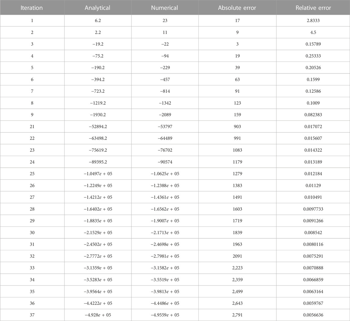
TABLE 1. Comparison of analytical solutions via the MSSE technique and numerical solutions computed via the modified VI technique for the model under investigation.

FIGURE 1

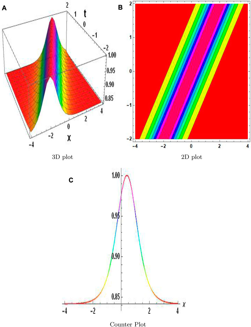
FIGURE 1. Physical depiction of v_1,1 at σ = 0.4, θ = −1.4, and η = 0.5.

FIGURE 2

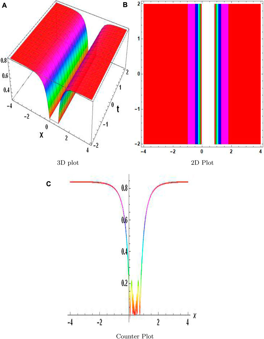
FIGURE 2. Physical depiction of v_1,2 at σ = 0.34, θ = −2.4, and η = 1.5.

FIGURE 3

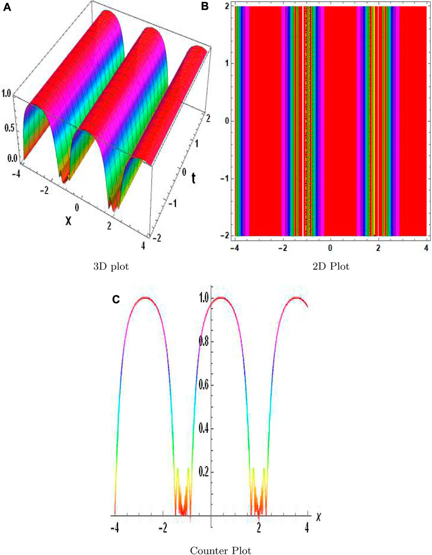
FIGURE 3. Physical depiction of v_1,3 at σ = −0.4, θ = 0.4, and η = −0.5.

FIGURE 4

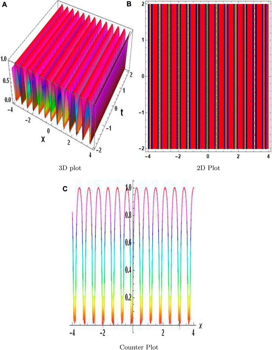
FIGURE 4. Physical depiction of v_1,4 at σ = 0.44, θ = −0.54, and η = 2.5.

FIGURE 5

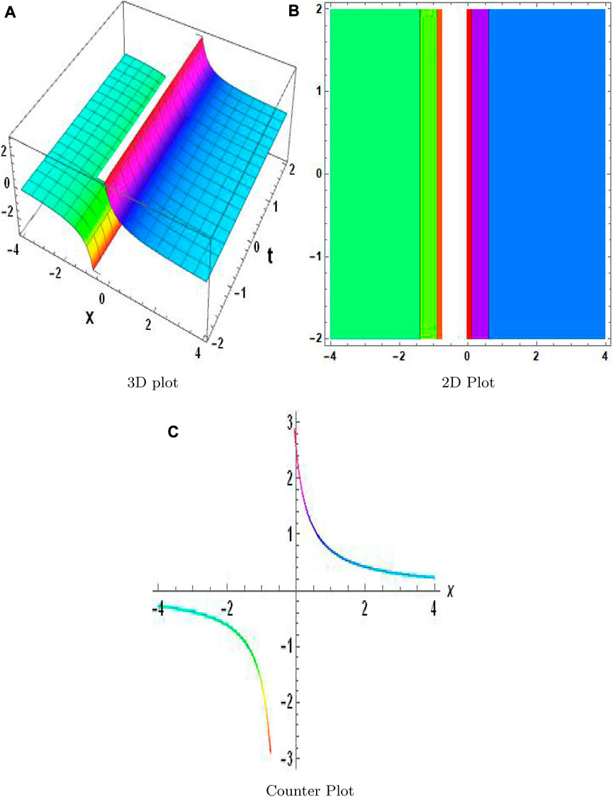
FIGURE 5. Physical depiction of v_1,5 at σ = 1.4, θ = −1.24, and η = 1.4.

FIGURE 6

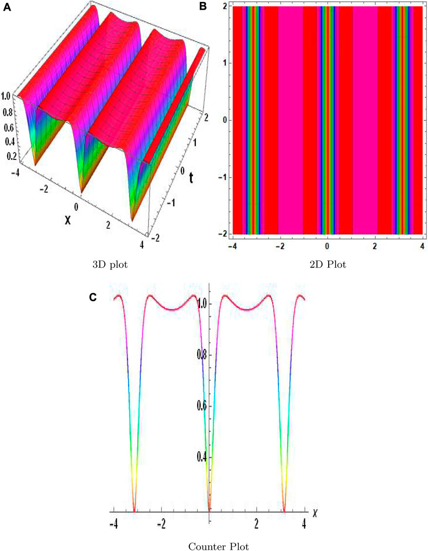
FIGURE 6. Physical depiction of v_2,1 at σ = −0.4, θ = −1.4, and η = −0.5.

FIGURE 7

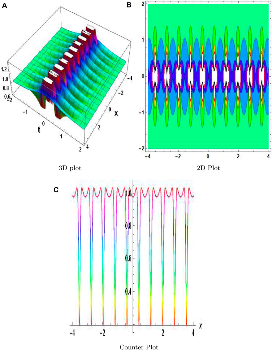
FIGURE 7. Physical depiction of v_2,2 at σ = 0.74, θ = −1.74, and η = 0.75.

FIGURE 8

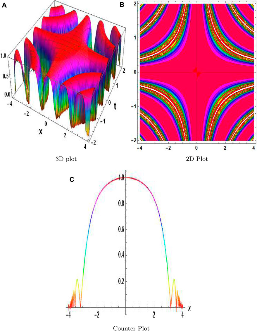
FIGURE 8. Physical depiction of v_2,3 at σ = 1.4, θ = −3.4, and η = 3.5.

FIGURE 9

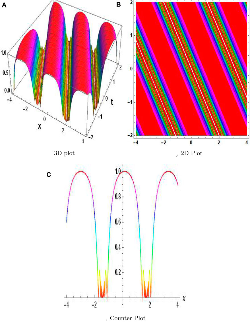
FIGURE 9. Physical depiction of v_2,4 at σ = −0.3, θ = −1.3, and η = 0.35.

FIGURE 10

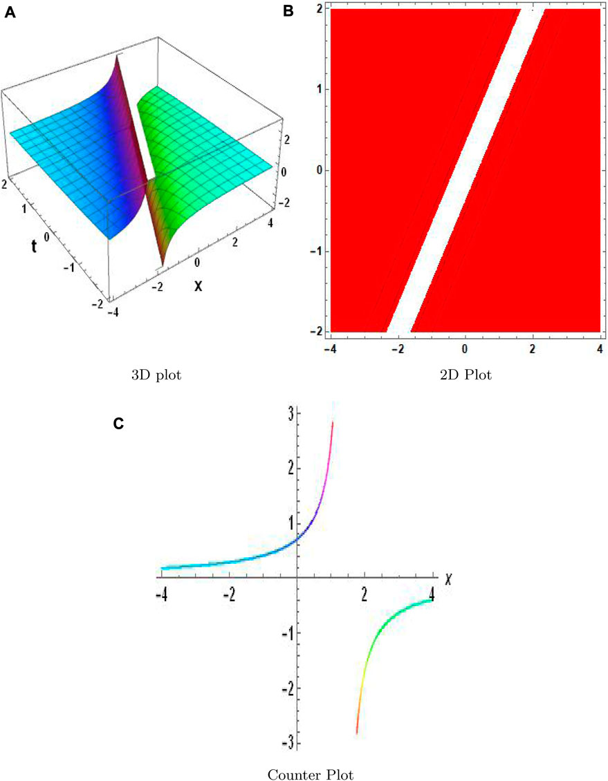
FIGURE 10. Physical depiction of v_2,5 at σ = 0.4, θ = −1.4, and η = 0.5. (A) is 3-D plot, (B) is 2-D plot, and (C) is contour plot.

FIGURE 11

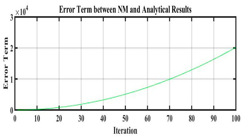
FIGURE 11. Comparison of error terms between numerical and analytical results by using values of Table 1.

FIGURE 12

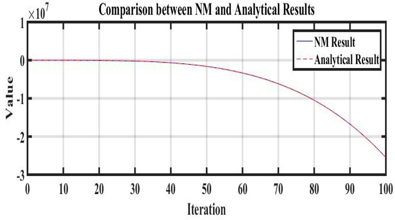
FIGURE 12. Comparison between numerical and analytical results by using values of Table 1.

FIGURE 13

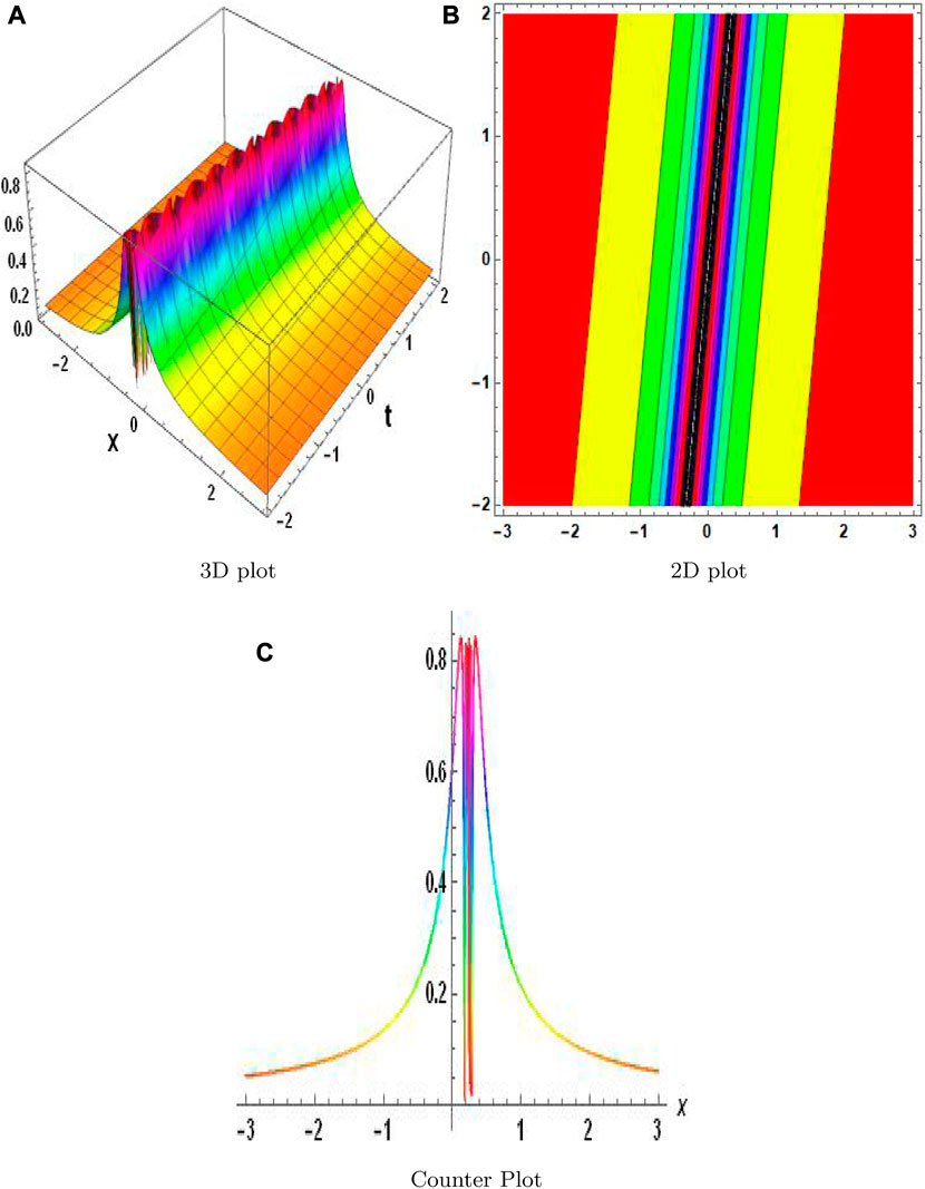
FIGURE 13. Physical depiction of H in Eq. 92 under σ = 0.5, v = 2.4, λ = 1.4, and ϑ = 0.4.

6 Conclusion

The nonlinear fractional Cahn–Hilliard and Gardner equations have been addressed in this paper using a unique methodology. This analytical technique is useful for creating partial differential equations and discovering approximate solutions under the right initial circumstances. The effectiveness of the suggested method is also shown by the precise results obtained utilizing MAEM with a smaller number of series terms. The application of this method to two different physical models demonstrates its accuracy and efficiency in handling fractional nonlinear equations, leading to stunning and complicated graphics. Additionally, the approximation series’ quick convergence is noted. We can see how the graphs change as a result of changing parameter values. When the calculations and simulations performed in Mathematica 11 were compared to previous numerical findings, it became clear that this numerical method is capable of handling difficult fractional equations in higher dimensions. The analytical approach used here is also notable for being straightforward, reliable, and succinct when solving nonlinear partial differential equations. The overall findings of the study emphasize the importance of this strategy in improving our knowledge and management of such difficult equations.

Data availability statement

The original contributions presented in the study are included in the article/Supplementary Material; further inquiries can be directed to the corresponding author.

Author contributions

AA: writing, conceptualization, formal analysis, supervision, and review and editing. AN: review implementation and editing. MN: formal analysis and review and editing. MJB: formal analysis and review and editing. AF: formal analysis and writing the original draft. AFA: formal analysis and review and editing. RH: formal analysis and review and editing. All authors contributed to the article and approved the submitted version.

Acknowledgments

The authors extend their appreciation to the Researchers Supporting Project (No. RSP2023R218), King Saud University, Riyadh, Saudi Arabia.

Conflict of interest

The authors declare that the research was conducted in the absence of any commercial or financial relationships that could be construed as a potential conflict of interest.

Publisher’s note

All claims expressed in this article are solely those of the authors and do not necessarily represent those of their affiliated organizations, or those of the publisher, the editors, and the reviewers. Any product that may be evaluated in this article, or claim that may be made by its manufacturer, is not guaranteed or endorsed by the publisher.

References

1. Ali A, Ahmad J, Javed S. Solitary wave solutions for the originating waves that propagate of the fractional Wazwaz-Benjamin-Bona-Mahony system. Alexandria Eng J (2023) 69:121–33. doi:10.1016/j.aej.2023.01.063

CrossRef Full Text | Google Scholar

2. Ali A, Ahmad J, Javed S. Exploring the dynamic nature of soliton solutions to the fractional coupled nonlinear Schrödinger model with their sensitivity analysis. Opt Quan Elect (2023) 55(9):810. doi:10.1007/s11082-023-05033-y

CrossRef Full Text | Google Scholar

3. Wang KJ. Traveling wave solutions of the Gardner equation in dusty plasmas. Results Phys (2022) 33:105207. doi:10.1016/j.rinp.2022.105207

CrossRef Full Text | Google Scholar

4. Kudryashov NA. Optical solitons of the model with generalized anti-cubic nonlinearity. Optik (2022) 257:168746. doi:10.1016/j.ijleo.2022.168746

CrossRef Full Text | Google Scholar

5. Wang KJ. Variational principle and diverse wave structures of the modified Benjamin-Bona-Mahony equation arising in the optical illusions field. Axioms (2022) 11(9):445. doi:10.3390/axioms11090445

CrossRef Full Text | Google Scholar

6. Ali A, Ahmad J, Javed S, Rehman SU. Analysis of chaotic structures, bifurcation and soliton solutions to fractional Boussinesq model. Physica Scripta (2023) 98:075217. doi:10.1088/1402-4896/acdcee

CrossRef Full Text | Google Scholar

7. Islam SR, Arafat SY, Wang H. Abundant closed-form wave solutions to the simplified modified Camassa-Holm equation. J Ocean Eng Sci (2022) 8:238–45. doi:10.1016/j.joes.2022.01.012

CrossRef Full Text | Google Scholar

8. Shakeel M, El-Zahar ER, Shah NA, Chung JD. Generalized exp-function method to find closed form solutions of nonlinear dispersive modified benjamin–bona–mahony equation defined by seismic sea waves. Mathematics (2022) 10(7):1026. doi:10.3390/math10071026

CrossRef Full Text | Google Scholar

9. Joseph SP. Exact traveling wave doubly periodic solutions for generalized double sine-gordon equation. Int J Appl Comput Math (2022) 8(1):42–19. doi:10.1007/s40819-021-01236-7

CrossRef Full Text | Google Scholar

10. Athron P, Fowlie A, Lu CT, Wu L, Wu Y, Zhu B. The W boson mass and muon g − 2: Hadronic uncertainties or new physics? (2022). arXiv preprint arXiv:2204.03996.

Google Scholar

11. Seidel A. Integral approach for hybrid manufacturing of large structural titanium space components (2022).

Google Scholar

12. Saifullah S, Ahmad S, Alyami MA, Inc M. Analysis of interaction of lump solutions with kink-soliton solutions of the generalized perturbed KdV equation using Hirota-bilinear approach. Phys Lett A (2022) 454:128503. doi:10.1016/j.physleta.2022.128503

CrossRef Full Text | Google Scholar

13. Liu SZ, Wang J, Zhang DJ. The fokas–lenells equations: bilinear approach. Stud Appl Math (2022) 148(2):651–88. doi:10.1111/sapm.12454

CrossRef Full Text | Google Scholar

14. Khater MM. Prorogation of waves in shallow water through unidirectional Dullin–Gottwald–Holm model; computational simulations. Int J Mod Phys B (2022) 37:2350071. doi:10.1142/s0217979223500716

CrossRef Full Text | Google Scholar

15. Muniyappan A, Sahasraari LN, Anitha S, Ilakiya S, Biswas A, Yıldırım Y, et al. Family of optical solitons for perturbed Fokas–Lenells equation. Optik (2022) 249:168224. doi:10.1016/j.ijleo.2021.168224

CrossRef Full Text | Google Scholar

16. He XJ, Lü X. M-lump solution, soliton solution and rational solution to a (3+ 1)-dimensional nonlinear model. Mathematics Comput Simulation (2022) 197:327–40. doi:10.1016/j.matcom.2022.02.014

CrossRef Full Text | Google Scholar

17. Zhang T, Li M, Chen J, Wang Y, Miao L, Lu Y, et al. Multi-component ZnO alloys: bandgap engineering, hetero-structures, and optoelectronic devices. Mater Sci Eng R: Rep (2022) 147:100661. doi:10.1016/j.mser.2021.100661

CrossRef Full Text | Google Scholar

18. Min R, Hu X, Pereira L, Soares MS, Silva LC, Wang G, et al. Polymer optical fiber for monitoring human physiological and body function: A comprehensive review on mechanisms, materials, and applications. Opt Laser Technolog (2022) 147:107626. doi:10.1016/j.optlastec.2021.107626

CrossRef Full Text | Google Scholar

19. Lechelon M, Meriguet Y, Gori M, Ruffenach S, Nardecchia I, Floriani E, et al. Experimental evidence for long-distance electrodynamic intermolecular forces. Sci Adv (2022) 8(7):eabl5855. doi:10.1126/sciadv.abl5855

PubMed Abstract | CrossRef Full Text | Google Scholar

20. Tarla S, Ali KK, Yilmazer R, Yusuf A. Investigation of the dynamical behavior of the Hirota-Maccari system in single-mode fibers. Opt Quan Elect (2022) 54(10):613–2. doi:10.1007/s11082-022-04021-y

CrossRef Full Text | Google Scholar

21. Ahmad J, Rizwanullah M, Suthar T, Albarqi HA, Ahmad MZ, Vuddanda PR, et al. Receptor-targeted surface-engineered nanomaterials for breast cancer imaging and theranostic applications. The Eur Phys J D (2022) 76(1):1–44. doi:10.1615/CritRevTherDrugCarrierSyst.2022040686

CrossRef Full Text | Google Scholar

22. Dubey S, Chakraverty S. Application of modified extended tanh method in solving fractional order coupled wave equations. Math Comput Simulation (2022) 198:509–20. doi:10.1016/j.matcom.2022.03.007

CrossRef Full Text | Google Scholar

23. Siddique I, Mehdi KB, Jarad F, Elbrolosy ME, Elmandouh AA. Novel precise solutions and bifurcation of traveling wave solutions for the nonlinear fractional (3+ 1)-dimensional WBBM equation. Int J Mod Phys B (2022) 37:2350011. doi:10.1142/s021797922350011x

CrossRef Full Text | Google Scholar

24. Jiang Y, Wang F, Salama SA, Botmart T, Khater MM. Computational investigation on a nonlinear dispersion model with the weak non-local nonlinearity in quantum mechanics. Results Phys (2022) 38:105583. doi:10.1016/j.rinp.2022.105583

CrossRef Full Text | Google Scholar

25. Bilal M, Rehman SU, Ahmad J. The study of new optical soliton solutions to the time-space fractional nonlinear dynamical model with novel mechanisms. J Ocean Eng Sci (2022). doi:10.1016/j.joes.2022.05.027

CrossRef Full Text | Google Scholar

26. Fu Z, Liu S, Liu S. New kinds of solutions to Gardner equation. Chaos, Solitons & Fractals (2004) 20(2):301–9. doi:10.1016/s0960-0779(03)00383-7

CrossRef Full Text | Google Scholar

27. Chen W, Sun H, Li XC. Fractional derivative modelling in mechanics and engeneering. Springer (2022).

Google Scholar

28. Abouelregal AE, Fahmy MA. Generalized Moore-Gibson-Thompson thermoelastic fractional derivative model without singular kernels for an infinite orthotropic thermoelastic body with temperature-dependent properties. ZAMM-Journal Appl Math Mechanics/Zeitschrift für Angew Mathematik Mechanik (2022) 102:e202100533. doi:10.1002/zamm.202100533

CrossRef Full Text | Google Scholar

29. Zhu Y, Tang T, Zhao S, Joralmon D, Poit Z, Ahire B, et al. Recent advancements and applications in 3D printing of functional optics. Additive Manufacturing (2022) 52:102682. doi:10.1016/j.addma.2022.102682

CrossRef Full Text | Google Scholar

30. Li Q, Shan W, Wang P, Cui H. Breather, lump and N-soliton wave solutions of the (2+ 1)-dimensional coupled nonlinear partial differential equation with variable coefficients. Commun Nonlinear Sci Numer Simulation (2022) 106:106098. doi:10.1016/j.cnsns.2021.106098

CrossRef Full Text | Google Scholar

31. Prakasha DG, Veeresha P, Baskonus HM. Two novel computational techniques for fractional Gardner and Cahn-Hilliard equations. Comput Math Methods (2019) 1(2):e1021. doi:10.1002/cmm4.1021

CrossRef Full Text | Google Scholar

32. Aniqa A, Ahmad J. Soliton solution of fractional Sharma-Tasso-Olever equation via an efficient (G′/G)-expansion method. Ain Shams Eng J (2022) 13(1):101528. doi:10.1016/j.asej.2021.06.014

CrossRef Full Text | Google Scholar

33. Khater M, Lu D, Attia RA. Dispersive long wave of nonlinear fractional Wu-Zhang system via a modified auxiliary equation method. AIP Adv (2019) 9(2). doi:10.1063/1.5087647

CrossRef Full Text | Google Scholar

34. Scarmozzino R, Gopinath A, Pregla R, Helfert S. Numerical techniques for modeling guided-wave photonic devices. IEEE J Selected Top Quan Elect (2000) 6(1):150–62. doi:10.1109/2944.826883

CrossRef Full Text | Google Scholar

35. Ali A, Ahmad J, Javed S. Stability analysis and novel complex solutions to the malaria model utilising conformable derivatives. The Eur Phys J Plus (2023) 138(3):259–17. doi:10.1140/epjp/s13360-023-03851-3

CrossRef Full Text | Google Scholar