 Shinichi Saito
95% of researchers rate our articles as excellent or good
Learn more about the work of our research integrity team to safeguard the quality of each article we publish.
Find out more
ORIGINAL RESEARCH article
Front. Phys. , 25 July 2023
Sec. Optics and Photonics
Volume 11 - 2023 | https://doi.org/10.3389/fphy.2023.1225360
Spin angular momentum of a photon corresponds to a polarisation degree of freedom of lights, and such that various polarisation properties are coming from macroscopic manifestation of quantum-mechanical properties of lights. An orbital degree of freedom of lights is also manipulated to form a vortex of lights with orbital angular momentum, which is also quantised. However, it is considered that spin and orbital angular momentum of a photon cannot be split from the total orbital angular momentum in a gauge-invariant way. Here, we revisit this issue for a coherent monochromatic ray from a laser source, propagating in a waveguide. We obtained the helical components of spin and orbital angular momentum by the correspondence with the classical Ponyting vector. By applying a standard quantum field theory using a coherent state, we obtained the gauge-independent expressions of spin and orbital angular momentum operators. During the derivations, it was essential to take a finite cross-sectional area into account, which leads the finite longitudinal component along the direction of the propagation, which allows the splitting. Therefore, the finite mode profile was responsible to justify the splitting, which was not possible as far as we were using plane-wave expansions in a standard theory of quantum-electrodynamics (QED). Our results suggest spin and orbital angular momentum are well-defined quantum-mechanical freedoms at least for coherent photons propagating in a waveguide and in a vacuum with a finite mode profile.
Newton recognised the polarisation degree of freedom in lights and called it as “sides” [1], whose properties were successfully elucidated by Stokes [2] and Poincaré [3] within the framework of classical mechanics [4–6]. Later, the discoveries of Plank and Einstein led to the establishment of quantum mechanics, and the wave-particle duality is unified in the form of a light quanta, a photon [7–10]. From a quantum mechanical point of view, the polarisation is understood as spin of a photon [8–10]. There are a lot of experimental evidences to believe that spin of a photon is 1 in the unit of Dirac constant, ℏ, which is the Plank constant, h, divided by 2π [7–10]. The most standard justification of spin 1 nature of a photon is the selection rule of absorption and emission of a photon by electrons in an atom [7–10]. Spin 1/2 nature of an electron and the integer quantisation of orbital angular momentum of electrons in a spherical potential are well-established, and the absorption and emission of a photon involves the change of ℏ in the orbital angular momentum of electronic states [7–10]. Spin 1 of a photonic state implies that there are potentially three orthogonal states, quantised along the direction of the propagation. However, a photon is propagating at the speed of light, c, in the vacuum, and it is described by a transverse wave. Consequently, electromagnetic fields of photons are oscillating perpendicular to the direction of the propagation, such that we can observe only two orthogonal polarisation modes and the spin 0 component is not observed [10]. As a result, the polarisation state of a photon [11–14] is described as a quantum-mechanical 2-level system using the SU(2) Lie algebra [4–6, 6, 8, 9, 15–27]. Therefore, it is natural to believe that a photon has inherent spin 1 as a quantum-mechanical degree of freedom.
It was rather recently that orbital angular momentum [5, 6, 28–33] of a light is considered in addition to spin. Allen and his co-workers demonstrated that the orbital angular momentum of the Laguerre-Gauss mode of a light is quantised in the unit of ℏ [28]. In their derivation, the classical electromagnetic wave in the Laguerre-Gauss mode under Lorentz gauge is used and the orbital angular momentum was calculated by using the classical Poynting vector, and the quantisation of electromagnetic fields as photons were taken into account at the end of the calculation to estimate the orbital angular momentum per photon [28]. In this pioneering work, they obtained that the orbital angular momentum of a photon is quantised in the unit of ℏ [28]. This suggests that the orbital angular momentum is also well-defined quantum-mechanical degree of freedom in addition to spin.
However, this native expectation is subsequently denied, because the gauge-independent expressions of spin and orbital angular momentum for photons were not obtained [29–31, 34, 35]. It is now generally believed that spin and orbital angular momentum of photons are not separately well-defined in a proper unique gauge invariant way [29–31, 34, 35]. More recently, it was successfully found that spin and orbital angular momentum operators are well-defined to satisfy the commutation relationship with the SO(3) symmetry in a gauge invariant way [36]. These previous works of quantum-field theories were based on plane wave expansions, which are suitable for most of many-body systems with translational and rotational symmetries, including black bodies, for which quantum mechanics was developed [7–10], and even more exotic systems like Quark-Gluon Plasma (QGP) [30]. Here, we will revisit this grand challenge for a monochromatic coherent ray of photons travelling in a waveguide, where rotational symmetry is spontaneously broken upon lasing. We are considering application in laser optic experiments [6], and therefore, we will work in a rest frame and we have not used the covariant formulation for relativity, which is important for high-energy physics such as Quantum Chromo-Dynamics (QCD) [30]. Nevertheless, we have employed the field theory of Quantum-Electro-Dynamics (QED), tailored to consider the Laguerre-Gauss mode in a GRaded-INdex (GRIN) fibre [6, 37]. We show that it is essential to consider the finite size of the mode profile to derive appropriate expressions for spin and optical angular momentum operators.
Fundamental understanding on the nature of spin and orbital angular momentum would be important for various applications of structured lights [38–43]. For example, it was experimentally demonstrated that an arbitrary spin state could be converted to the properly designed superposition state of orbital angular momentum [44], and this experiment suggests that the orbital angular momentum state is well-defined with the polarisation state, so that spin and orbital angular momentum must be equally qualified observables. It is also interesting to consider the light-matter interaction and the corresponding selection rule with the orbtial angular momentum [41]. It was shown that the dipole selection rule is not significantly affected by orbital angular momentum, while orbital angular momentum of lights could be transferred to the orbital of an excited electron in a quantum dot [41]. The conservation law of total angular momentum is also important in silicon photonic devices, and we have previously shown that the quantum number of spin and orbital angular momentum emitted from the micro-gear must be determined by the number of gears and the number of nodes in the ring [45]. For high-speed fibre-optic communication, orbital angular momentum will expand the bandwidth significantly, and technologies for multiplexing and de-multiplexing are important [40, 46]. Among many other applications, we think it is exciting to explore macroscopic quantum coherency among various superposition states with orthogonal spin and orbital angular momentum states, known as classically entangled states [38–43]. In order to explore the potential use of these states for quantum computing and/or quantum simulation [47], we have examined how spin and orbital angular momentum are represented based on a quantum field theory.
Before showing our final results, we start from classical results for electromagnetic waves and adding some complexities gradually to address what was the potential issue [5, 6, 28–33]. First, we confirm orbital angular momentum described by a Laguerre-Gauss mode in a free space under the Lorentz gauge [28]. Then, we confirm that the same result can be obtained by using the Coulomb gauge and compare the difference of gauges. We also confirm the impacts of polarisation on optical angular momentum by using a horizontally polarised mode and a circularly polarised mode. Finally, we extend the analysis for the GRIN waveguide for both polarisations.
Here, we consider a uniform transparent material with the dielectric constant of ϵ and the permeability of μ0. The velocity of the light in the material is given by
The electric field, E, and magnetic induction, B, are obtained by
respectively, which immediately gives the electric displacement field D = ϵE and the magnetic field H = B/μ0. We can confirm that Maxwell equations [5],
in the absence of the charge ρ = 0 and the current J = 0 are satisfied under the Lorentz gauge by directly inserting Eqs 4, 5.
We consider an electromagnetic wave in a Cartesian coordinate. From Maxwell equations, we obtain the Helmholtz
A particular solution, polarised along the horizontal direction is
where r = (x, y, z) is the Cartesian coordinate, z is the axis along the direction of the propagation,
and the Helmholtz equation becomes
which is the same form with the non-relativistic Schödinger equation [8, 9, 52–54]. A particular solution, which is separable in a cylindrical coordinate [6, 28], is obtained as
where
In the mode profile of ψ(r, z), the phase factor of eimϕ is very important to describe the optical orbital angular momentum of ℏm [28]. Another important feature of the Laguerre-Gauss mode is the Gouy phase [28, 52, 55–59]
The phase of the Laguerre-Gauss mode as a scalar field of ψ(r, z) is given by
We consider the gradient of the phase in the cylindrical coordinate (r, ϕ, z)
where the unit vectors along r and ϕ are obtained by a rotation of the unit vectors in (x, y) coordinate (Figure 1) as
In particular, it is important to be aware that the unit vectors
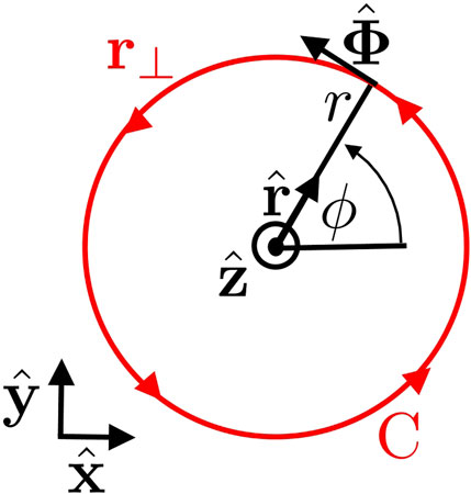
FIGURE 1. Topological charge by optical angular momentum. The contour integral along the closed circle C in a cylindrical coordinate (r, ϕ, z) is considered, which gives the winding number, called the topological charge. Note that the existence of the node at the origin is required to support the topological charge. We assume that the light is propagating along z and the direction of rotation is defined to be positive, if the rotation is anti-clock-wise seen from the top of the z-axis in the detector side. In this definition, the left-circular vortexed state, shown above, corresponds to the positive winding number, corresponding to the quantised optical angular momentum pointing towards the positive z direction.
We consider the contour integral for the closed path C (Figure 1) for the gradient of the phase as
which is the winding number, called the topological charge. Please note that I is the dimensionless number, such that it is confusing to call it as charge. The winding number would be a more precise word, instead. Nevertheless, the existence of the finite I is responsible for twisting lights to form a vortex with optical angular momentum, such that it works like a source of generating a vortex of the electric field, similar to charge, which is the source of divergence of the electric field. In order to sustain the vortex, it is essential to have a node within the inside of the contour, C. Otherwise, the integration of the gradient simply becomes zero as
in the limit of closed integration circle, r1 → r0. This means that there is a node required at the centre of the beam in order to sustain non-zero topological charge, which is guaranteed in the Laguerre-Gauss mode with a power of r|m| for m ≠ 0. Please also note that there is no singularity in the electric field but there is a node (zero point). In other words, the amplitude becomes zero, such that it is impossible to define a phase at the node. Therefore, we can also claim that there is a singularity in the phase, if we try to define the phase at the node. This is consistent with the view that we should not expect singularities in observables like electric and magnetic fields. The topological charge simply corresponds to a node.
Another important source of an unnecessary confusion is the definition of the direction of the rotation of the vortex. Depending on whether we are observing the vortex from the detector side or from the source side, the rotation will become opposite. In our paper, we define the positive rotation for the left-circular vortex, seen from the detector side, which corresponds to the positive topological charge, m > 0 (Figure 1). We usually use the right-handed coordinate for Cartesian coordinate of (x, y, z), and we are assuming that the light is propagating towards the positive z direction. In the descriptions of the rotation of the vortex and the polarisation ellipse, we think it is natural to describe in the (x, y) plane, seen from the top of the z-axis, corresponding to seeing from the detector side for a ray pointing towards z (Figure 1). In the cylindrical coordinate, a standard definition of the angle ϕ is measured from the x-axis in the anti-clock-wise direction, such that x = cos ϕ and y = sin ϕ. In this coordinate, the left-circulation (anti-clock-wise) of the contour corresponds to the positive topological charge, and we will confirm that this corresponds to the quantised orbital angular momentum of
Similar to the polarised lights, we would like to propose to call as vortexed lights for the ray with a vortex of non-zero topological charge.
The time dependence of the ray, we are considering in this paper, is simply described by e−iωt. Strictly, both E and B must be real, since these are observables but it is easier to use complex valuables, instead, and to make a convention to take the real part at the end of the calculations [6]. In this convention, it is important to take a factor of 2 for the products, because the time average of cos2(ωt) or sin2(ωt) must be 1/2. This is important when we consider the momentum of the electromagnetic wave
and the Poynting vector
whose time averages are obtained as
and
respectively. The Poynting vector describes the flux flow of the energy by photons, such that
where
Next, we consider the horizontally polarised Laguerre-Gauss mode in Lorentz gauge [28] using the vector potential,
where the total mode profile and the propagation is described by the wavefunction
In this case, we obtain B and E as a function of A = (A, 0, 0). It is straightforward to obtain
where we have abbreviated as ∂x = ∂/∂x, ∂y = ∂/∂y, ∂z = ∂/∂z, and ∂t = ∂/∂t. The Lorentz condition becomes
from which we obtain
Then, we obtain
In the paraxial approximation, we can neglect as
and we use
For the calculations of Poynting vector and the momentum, we calculate
which yields
where
The naive expectation value of the momentum would be
Thus, we obtain
Therefore, we realise that the vector potential is essentially an wavefunction. In fact, it can also be re-written as
This expression is very similar to a probability flux for a wavefunction [7–10, 28]. For taking the time average, it becomes
for which we expect the relationships, |E0| ≈ ω|A0| and
The dominant contribution of this value becomes
If we accept the coherent monochromatic light is quantised as photons, the average energy density simply becomes the ratio between the number of photons
which immediately yields
This means that the total momentum density of the electromagnetic wave is the sum of the contributions from photons per unit volume, and each photon has the momentum of p = ℏk. This is also consistent with the Bose-Einstein condensation nature of the coherent ray of photons from a laser source, because the coherent photons occupy the same energy and momentum state.
In the above estimation, we have not considered the mode profile, coming from the Laguerre-Gauss mode, such that we calculate
in more detail. To do so, it is better to move to use the cylindrical coordinate. The derivatives are converted to be
for which we use
and
Then, finally we obtain
where we can also use the Plank’s law for the quantisation of photons,
After obtaining the momentum density, we can proceed to estimate orbital angular momentum, which is naturally expected as [28]
for which we can also use the quantisation condition to obtain
This means that the major component of the optical orbital angular momentum is along z direction, which is given by
We can also calculate the magnitude of the optical orbital angular momentum density as [28]
In the previous subsection, we have confirmed the original approach using the Lorentz gauge [28] for the preparations. The results should not be dependent on the arbitrary choice of the gauge. Here, we use the Coulomb gauge to confirm it.
In the Coulomb gauge [5], the vector potential satisfies the transversality condition
which yields
One might naively think that the horizontally polarised Laguerre-Gauss mode is described by
however, this is wrong because this does not satisfy the transversality condition due to the r and ϕ dependences of the vortexed mode (∂xA ≠ 0 and ∂yA ≠ 0).
The correct form for the Coulomb gauge would be
which is the same form for that in the Lorentz gauge. Therefore, the small finite longitudinal component is responsible for guaranteeing the gauge-invariant solution. Consequently, the vector potential in the Coulomb gauge is described as
which is obviously different from that in the Lorentz gauge due to the existence of the longitudinal component of Az. We can double check that this satisfy the transversality condition, directly by calculating
By using the vector potential and vanishing scalar potential in the Coulomb gauge, we obtain the same formulas for E and B, compared with those obtained in the Lorentz gauge. Therefore, A and Φ could depend on the choice of the gauges, while the observables such as E and B cannot be dependent [5]. The differences of the gauges are summarised in Table 1. In particular, the inclusions of the small longitudinal fields are indispensable for the considerations of the orbital angular momentum due to the spatial dependence of the mode profile. This is a remarkable difference compared with the simple plane-wave expansion without considering the mode profile in the most of the theory of QED [7, 10, 29–31, 34–36]. This is one of the key considerations to enable the splitting of spin and orbital angular momentum, as we shall see in due course.
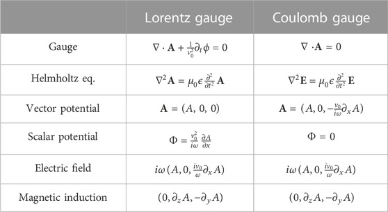
TABLE 1. Summary of fields in different gauges. The horizontal polarisation is assumed.
Before we continue to consider the full quantum field theoretic treatment, it is further worth for learning from the historical work [28] for circularly polarised mode, because this shows how spin could appear in optical angular momentum. Here, we will go back to the Lorentz gauge [28], because now we understand that the choice of the gauge should not affect the final result at all.
For circularly polarised Laguerre-Gauss mode, we assume
where σ = σz corresponds to the quantum number for spin pointing to the direction of the propagation (z). Usually, a circularly polarised state is defined by a transverse electric field, and we will in fact confirm that the above postulate for a vector potential is consistent with the calculated electric field as a circularly polarised state. In our preferred notation, shown in Figure 1, the left-circularly polarised state corresponds to the anti-clock-wise rotation of the polarization circle, seen from the detector side, which corresponds to σ = +1 and spin angular momentum along z for the photon is +ℏ. The right-circulary polarised state rotates clock-wise, which corresponds to σ = −1 and spin angular momentum per photon is −ℏ. A = A(r, ϕ, z) = A0Ψ(r, ϕ, z) = A0u(r, z)eimϕei(kz−ωt) is described by the Laguerre-Gauss mode, such that we have spatial profile with the non-zero derivatives.
It is straightforward to obtain the magnetic induction as
From the Lorentz condition, we obtain
which gives
In the paraxial approximation, we calculate
and together with ∂tA = −iωA, we obtain
Here, we confirm that the transverse electric field of (Ex, Ey) is consistent with the assumed circular polarisation as Ey/Ex = iσ. The small longitudinal component of Ez plays an essential role for splitting spin and orbital angular momentum, as we will see below.
Then, we can proceed for calculating the momentum and the optical angular momentum. First, we calculate
where the spin independent term is coming from the orbital component, which is the same as that in the horizontally polarised mode and is proportional to
For them, we evaluate the derivatives,
which will cancel each other for
and we also use the identity
Finally, we obtain
This gives the angular momentum contribution from spin as
By averaging over the cross section, x and y components vanish, and we calculate
where we use the normalisation condition
and we obtain [28]
Therefore, the circular polarised ray carries the spin angular momentum, and the single photon contributes with the amount of ℏσz along the direction of the polarisation. In our convention (Figure 1), the left-circularly polarised photon (σz = +1) brings ℏ, while the right-circularly polarised photon (σz = −1) brings −ℏ [28], as we expected.
Next, we consider a GRIN fibre [6, 37], which has a quadratic dependence of the dielectric constant profile on r, described as
We continue to use the Lorentz gauge in this subsection, and the Helmholtz equation in a GRIN fibre becomes
For the horizontally polarised mode, the solution would be in the form of
where the beam waist becomes constant,
where δω0 = v0g. The radius of the spherical phase diverges, R → ∞, so that the beam is perfectly collimated to propagate in a GRIN fibre for a long distance without focussing or de-focussing within the fibre. The important point, here, is that the profile of the Laguerre-Gauss mode works as an envelop function, ψ(r, ϕ, z), against the total wavefunction, Ψ(r, ϕ, z). In the simple plane-wave expansion, the approximation of ψ(r, ϕ, z) → 1 is employed, but this is not acceptable when we consider the orbital angular momentum, due to the vortexed beam shape with a node, characterised by topological charge.
The Lorentz condition becomes
By inserting the horizontally polarised form, A = (A, 0, 0), we obtain
which gives
Therefore, we can approximate
We also obtain
Then, we can proceed for calculating the momentum and angular momentum. For that, we need to estimate
By evaluating derivatives,
we obtain
Using the quantisation of the energy for photons, we obtain
Finally, we obtain the angular momentum
For the circular polarised state, we can follow exactly the same procedure to obtain the spin contribution to the angular momentum as
These results are the same as those obtained by taking the limit of R → ∞ in the formulas obtained for the free space.
In the previous section, we have confirmed the important discovery of Allen and collaborators for optical angular momentum [28]. While it was intriguing to obtain the quantised angular momentum, solely by accepting the fact that the energy of the optical ray is quantised as a photon at the end of the calculation, it is not conclusive whether spin and orbital angular momentum are really fundamental quantum degrees of freedom of photons or not [5, 6, 28–36]. In particular, it is highly questionable whether we can derive a full quantum-mechanical expression solely by using Poynting vector and the classical expectation for the angular momentum,
First, we clarify the problems of using plane-waves for the description of the coherent monochromatic ray of photons emitted from a laser source. Historically, the quantum mechanics was developed to explain black-body radiation, such that it would be natural for physicists at that time to consider photons of all possible modes under thermal equilibrium with the Plank distribution function at finite temperature [7–10]. Therefore, a standard theory of QED is based on the plane-wave expansions of the field, imposing the commutation relationship to field operators as Bosons for photons [7–10]. However, photons are barely interacting each other due to the absence of charge, and a coherent ray of photons from a laser source is described by a single mode [6, 32, 60] essentially similar to the Bose-Einstein condensation, in a sense that the macroscopic number of photons are occupying the same state. Due to the absence of the Coulomb interaction between photons, photons can be treated purely quantum mechanically without considering the ensemble average [10, 32, 60], such that the temperature for photons emitted from a laser are equivalent to zero temperature, even if the measurements are conducted at room temperature.
In that sense, it would be not suitable for light from a laser by using a plane-wave for discussing the nature of orbital angular momentum. Even lights from Sun are not spreading to the entire universe like plane-waves, and lights are predominantly propagating along uni-direction with finite spreading as wave-packets. Moreover, the plane-wave cannot sustain the vortexed lights, as we have shown in the previous section due to the lack of the node at the centre of the vortex. Even without the orbital angular momentum (m = 0), the plane-wave description is not suitable for the light propagating with the finite mode profile for discussing the nature of spin of photons, as we shall see below. Plane-waves are suitable for extended states, spreading to the entire system, while lights propagating in a waveguide are trapped in bound states. Nevertheless, in this subsection, we intentionally use the plane-wave to understand what was the problem to elucidate the nature of the angular momentum of photons.
In this subsection, we explain our notation on the use of the quantum field theory for photons. The use of the plane wave corresponds to the flat nodeless mode profile, which spreads the entire volume of the system, which is described by an envelop function
and the full single wavefunction for a photon is
where β = kz − ωt + β0 describes the standard phase evolution for a photon, propagating along z and β0 is the arbitrary U(1) global phase. Here, we consider a propagation in a uniform material, such that the dispersion is ω = v0k. The normalisation over the volume, V, is included in
whose complex conjugate (adjoint) is
where
where σ and σ′ describe the polarisation, and δσ,σ′ is the Kronecker delta, which gives 1 for the same mode and 0 for the orthogonal mode.
The observable electric field operator is given by
which always satisfy the transversality condition
One would recognise that this is already a big problem when we consider orbital angular momentum, because of the lack of the small longitudinal component along z (Table 1), which was responsible to guarantee the gauge condition. Nevertheless, let’s continue to see what happens to spin angular momentum under the plane wave expansion. Please also note that we have not summed up over all possible electromagnetic modes in a waveguide, because we are considering a single mode of a monochromatic coherent ray from a laser source.
The transversality condition for the Coulomb gauge,
which gives the amplitude of the vector potential per photon,
The magnetic induction operator is calculated as
This corresponds to the average amplitude of the magnetic induction of
We think it is worth for clarifying our definition of the polarisation for electromagnetic waves (Figure 2). As we explained in Figure 1, we define our rotation seen from the detector side, and the positive rotation is for the anti-clock-wise direction. The electric field and magnetic induction operators are summarised as
where the components of the electric field operator are defined as
The relative vectorial relationships are schematically depicted in Figure 2. In our definition, the vectorial direction of the magnetic induction is obtained by rotating the electric filed with the amount of 90° along z. The 90°-rotation of the electric field corresponds to the application of the optical rotator, which rotates the polarisation state described by Jones vector on the Poincaré sphere with the amount of 180° along S3, which converts the horizontal linear polarisation to the vertical one or the diagonal linear polarisation to the anti-diagonal one, while keeping the circular polarised states for both left and right circulations.
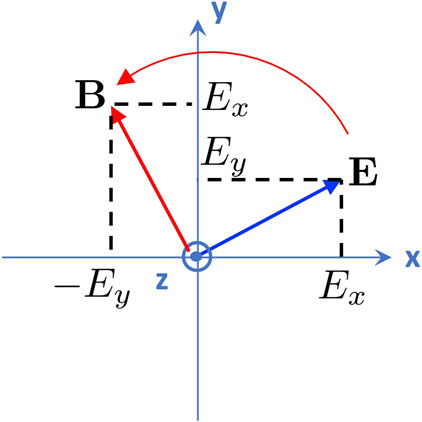
FIGURE 2. Orthogonality between electric and magnetic fields. The vectorial direction of B is obtained by rotating E with the amount of 90° along z.
The Hamiltonian is expected to be
Upon inserting field operators,
which is equivalent to the longitudinal phase-matching condition k = 2πn/L with an integer
and the spatial integration gives the volume V = LxLyLz, which will be cancelled with the contribution from
where zero-point fluctuations of ℏω/2 per polarisation degree of freedom are successfully included.
The momentum density operator for photons is given by
where the Ponynting vector operator is
The integrated total momentum operator becomes
where the zero-point oscillations are included. If we consider a ray, propagating in an opposite direction, the zero-pint oscillations cancel each other among photons with +k and −k.
Then, we proceed to calculate the angular momentum operator
using plane-wave basis. We use identities [5],
and split the total angular momentum operator [29–31, 34–36] into the orbital angular momentum operator
where
and
But, this is not extremely successful, because
due to the odd parity symmetry of x and y against the origin, while
due to the same argument on the parity symmetries of the integrand. Moreover, if we continue to use
where the first term might vanish [30, 34, 35], if we consider the mode vanishes at the boundary of the waveguide. The tactic of the introduction of the vanishing boundary condition [30, 34, 35] can be justified, if we consider a mode profile, which is not properly taken into account for plane-waves. Then, we obtain the only finite component along the direction of the propagation (i = z),
which apparently depends on the choice of the gauge [29–31, 34, 35]. We obtained this expression by using the Coulomb gauge, and one might be able to justify to take only the transversal component of the vector potential to justify this formula [29, 31]. However, it is still questionable to retain the finite operator contribution, which has vanished in the symmetry argument. Nevertheless, if we continue to proceed to express
which makes reasonable sense [29]. Although the derivation, we have confirmed, in this subsection is not acceptable, the final result is intriguing.
Next, we show that the problems were coming from the choice of the expansions of the field by plane-waves. Our goal is to justify the splitting between spin and orbital angular momentum and to get more insights for obtaining full quantum operators for spin and orbital angular momentum. We will achieve this goal by using a Laguerre-Gauss mode and a standard quantum-field theory for a vortexed coherent monochromatic ray.
We must develop a quantum field theory for a coherent monochromatic ray for photons, propagating in a waveguide. Therefore, we need to take topological charge into account for allowing the vortexed beam with a specially non-trivial profile. In order to make the argument based on a specific example, we consider a GRIN fibere, but the application to the other waveguide will be straightforward. Here, we consider the fundamental principle to develop the theory.
First, we consider a monochromatic coherent state for photons [32, 60, 61],
where σ describes the polarisation state such as horizontal (H) and vertical (V) states. ασ is a complex number, which we will obtain, soon. We can also choose other combinations of orthogonal states such as diagonal (D) and anti-diagonal (A) or left (L) and right (R) polarised states. The quantum mechanical expectation value of the number operators by the coherent state becomes
where
which is obtained by assigning
where α is the auxiliary angle to split
The electromagnetic field, expected from the coherent state, must be compatible with Maxwell equations and, thus, with the Helmholtz equation. Both the electric field and the magnetic field are observalbes and obtained by taking the quantum-mechanical expectation values by the coherent state. The dominant contribution for the complex electric field becomes
where Ψ(r, t) works as a wavefunction to describe the orbital part of photons. If we take quantum-mechanical average of
where
which describes the spin state of photons [6, 11, 12].
As we have shown in the previous sections, the results should not depend on the choice of the gauge. We will chose the Coulomb gauge, such that E(r, t) should satisfy the Helmholtz equation (Table 1), which is equivalent to imposing Ψ(r, t) to satisfy the Hemholtz equation,
This means that the orbital wavefunction of a photon is described by the Hemholtz equation rather than the Schrödinger equation. In a free space, this simply gives the plane-wave, but in a material with the spatial profile of the dielectric constant, the solution can be highly non-trivial, depending on the symmetry of the system and boundary conditions. For a monochromatic ray, we can assume a simple Plank-Einstein relationship of E = ℏω, such that the wavefunction is described by a single mode of the angular frequency of ω as Ψ(r, t) = Ψ(r)e−iωt, and we obtain
In a GRIN waveguide, we can assume
In the cartesian coordinate, we can assume
which gives the Hermite-Gauss mode [6]
where
In a cylindrical coordinate,
which gives the Laguerre-Gauss mode
The dispersion relationship for the Hermite-Gauss mode is given by a frequency shift, δw0 = v0g, as
and the corresponding equation for the Laguerre-Gauss mode is obtained by replacing l = 2n and m → |m|. This can be rewritten by using the Plank-Einstein relationship for the energy (E = ℏω) and momentum (p = ℏk) of a photon,
which yields
where the energy gap Δ is
which implies that the photon confined in a waveguide is massive due to the broken symmetry [62–65]. The mass increases with the increase of the orbital angular momentum m and the radial quantum number of n. In a weak coupling limit (g → 0), the effective mass of m* vanishes. We should choose the solution of the positive energy for the confined mode, propagating the waveguide, and thus we obtain
Below, we will focus on the Laguerre-Gauss mode with a cylindrical symmetry. We normalise the wavefunction as
and the normalised solution becomes
where the volume is given by
Now, we will examine the complex electric field operator in more detail. According to our classical considerations for a Laguerre-Gauss beam, it was essential to take the small longitudinal component for ensuring the vortexed beam sustained by topological charge. This corresponds to add the longitudinal component,
for obtaining a self-consistent result in the Coulomb gauge (Table 1), for which
must be satisfied. The latter corresponds to the identity for the complex vector potential operator,
By inserting this into
which gives the longitudinal component of the operator as
where we have used
which is valid in the weak confinement limit, g → 0.
Consequently, we obtain
whose conjugate becomes
The electric field operator is also obtained as
whose quantum-mechanical expectation value must always be real, which is guaranteed by
On the other hand, the conjugate of the complex vector potential operator satisfies
which yields
This satisfies the transversality condition of the Coulomb gauge
It is also straightforward to calculate
by assuming
which guarantees that the magnetic induction is also observable,
(Figure 2) is also satisfied for a vortexed beam, because
By using the obtained
where we have used
By taking the quantum-mechanical average using the coherent state, we obtain the total energy of photons,
and the energy density of the electromagnetic waves becomes
where the photon density is given by
We define the complex momentum operator,
whose conjugate is
Therefore,
is observable, because
whose average over space becomes
The major component along z is obtained as
as we expected. In a similar way, we calculate
where the last term of Ψ*∂yΨ + Ψ∂yΨ* will be cancelled when we calculate
We can simplify the integrands as
and
Then, we obtain
We obtain
Similarly, we calculate
and then, we obtain
for which, we calculate the integrands,
and
Then, we obtain
whose integrand becomes
If we move to the cylindrical coordinate (r, ϕ, z), we obtain the momentum-density operators
Finally, we can calculate the angular momentum-density operators by assuming
In the Cartesian coordinate, (x, y, z) = (r cos ϕ, r sin ϕ, z), we obtain
where we have used
at the last line.
In the cylindrical coordinate,
where the last line is especially important, since we finally obtained orbital and spin angular momentum operators
respectively.
When we integrate over space, we realise
Thus, we obtain
For the angular momentum operator, defined by
we obtain
where
For the spin operator, the number operators of left and right circular states are used, which are defined as
and
Here, we could split the total angular momentum operator into orbital and spin angular momentum operators without the apparent gauge dependence. We could perform a gauge transformation for photons, but due to the absence of charge for photons, the gauge field will not couple to the change of the angular momentum operators. The gauge independence is obvious in our expressions, because the number of photons should not depend on the choice of the gauge, otherwise the total energy of the system can change depending on the arbitrary choice of the gauge.
It is interesting to be aware that there exists contributions from zero-point oscillations in the orbital angular momentum for a ray propagating towards one direction. Such a zero-point fluctuation is absent for spin. We do not know exactly why a zero-point fluctuation has not been appeared for spin. But, spin is an internal degree of freedom for photons, which can never be removed. On the other hand, orbital angular momentum (m ≠ 0) could be suspended, if the waveguide is small enough to allow only the single mode. In such a single mode waveguide, the zero-point fluctuation can also be suppressed. However, as far as the waveguide allows the higher order mode with non-zero orbital angular momentum, the zero-point fluctuation must be remained. Another possible reason is found in the expression of calculated spin and orbital angular momentum. The orbital angular momentum is expressed as the sum of numbers of photons in 2 orthogonal polarisation states
Another interesting point is that we could obtain only the angular momentum operators along the direction of the propagation from simple analogy from the classical counter part defined by
Before proceeding to consider the full orbital angular momentum operators, further, in this section, we discuss the origin of the photonic spin angular momentum for a coherent monochromatic ray without an orbital angular momentum in a general waveguide (Figure 3). Spin of a photon is an inherent quantum degree of freedom, which should be described quantum-mechanically rather than classically. In the absence of the orbital angular momentum (m = 0), we should not have any issue to regard the total angular momentum is exclusively coming from spin. Therefore, the situation would be simpler than the splitting of spin and orbital angular momentum. We check the derivation of the last section for the case of m = 0 in detail to understand spin of photons.
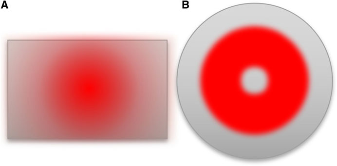
FIGURE 3. Examples of waveguides of (A) a rectangle shape and (B) a cylindrical shape. The mode profile is essential to confine lights inside waveguides, so that a plane-wave cannot be a good approximate mode. The Gaussian profile is used to describe the Hermite-Gauss mode for the strip waveguide (A) and the Laguerre-Gauss mode for (B) in a GRIN waveguide.
For photons propagating in a waveguide, it is essential to take the mode profile [6] into account, which means |∂rΨ| ≠ 0. On the other hand, we will employ the paraxial approximation,
From the Coulomb gauge condition,
we obtain the longitudinal component,
which was not considered in the plane-wave expansions. The existence of this small longitudinal component is responsible to obtain the spin angular momentum operator, properly. Then, we obtain the same expression for
On the other hand, in the absence of the angular orbital momentum, the mode profile is described by a real function,
which correspond to
in a Cartesian coordinate, and
in a cylindrical coordinate.
Then, we calculate
in a Cartesian coordinate, and
After the integration, finally, we obtain
as before, while
where the total angular momentum along z is solely described by the spin angular momentum
as we expected, and the orbital angular momentum vanishes. We also confirmed that the final result depends solely on the difference of number of photons between left and right circularly polarised photons, such that
In the previous sections, we have obtained the spin operator only along the direction of the propagation as,
where
Here, we impose the principle of rotational invariance for photonic polarisation states to describe the propagation in a waveguide with a cylindrical symmetry or a free space. We know that there exists two orthogonal polarised states for describing the photonic state, and we choose left and right circularly polarised states as basis states, for example. Then, we use SU(2) Lie-Algebra [66], and spin should work as a generator of rotation [7–10],
where
which satisfy the commutation relationship
Then, we obtain
Similarly, we obtain
We also define
to account for the total number of coherent photons for each polarised components. This also accounts for the time averaging of incoherent lights, which we are not discussing, here.
The general polarisation coherent state in the chiral basis is described by Bloch state [7–10]
where θ is the polar angle and ϕ is the azimuthal angle. By taking the quantum mechanical average of spin operators
which means that the Stokes parameters [11–14, 16–20, 67, 68] to describe the polarisation state of coherent photons were actually the quantum-mechanical expectation values of spin for photons.
We can also go back to the original horizontal-vertical (HV) basis by the unitary transformation, which we obtained from the classical correspondence using
where
and
We can also re-write
The quantum mechanical expectation values using coherent state of |αH, αV⟩ are immediately calculated as
We can also use the Jones vector to calculate the spin expectation values by using the coherent state, and we obtain
which is consistent with the above results obtained in the chiral representation. The spatial components of Stokes parameters, S = (S1, S2, S3), are usually shown in Poincaré sphere. In the Jones vector description, the polar angle γ = 2α is measured from S1 axis and the azimuthal angle δ is measured from S2 in the S2-S3 plane.
We can also confirm the sum rule
for the expectation values in the coherent spin states.
We also obtained the commutation relationships [16–20, 67, 68] for spin operators as
which are valid for both chiral and Jones bases. Therefore, we obtained the spin operators for all components as generators of rotations for polarisation state of a coherent monochromatic ray of photons.
Now, we are ready to discuss what was
The helicity operator naturally sets the direction of the quantisation axis of spin aligned to the direction of the propagation. Nevertheless, this does not exclude the other polarisation states nor the spin components, perpendicular to the direction of the propagation. The spin expectation values are observables, as clearly established as polarimetry [11, 12]. Please also note that the expectation values of spin components are independent on the value of the quantum orbital angular momentum, m, because we have allowed the vortexed ray with non-zero topological charge. In that sense, our results show that the spin angular momentum is independent on the orbital angular momentum. Therefore, our framework is a natural extension of a standard QED theory to account for the spatial profile of the orbital wavefunction of photons, and we found that the spin angular momentum was not affected by the orbital angular momentum.
It is amazing to consider why Stokes and Poincaré [2–6] could establish the descriptions of polarisation states using these parameters before the discoveries of quantum mechanics and the quantum field theories. It is also astonishing to be aware that Stokes and Poincaré [2, 3] properly assigned the correct order parameters
Now, we will extend our discussions for quantum-mechanical nature of orbital angular momentum for photons. In order to make the argument specific, we consider a GRIN fibre under a cylindrical symmetry, again, but the extension to a more general waveguide is straightforward, as we discussed in sections for obtaining spin operators. In the preceding sections, we obtained the orbital angular momentum along the direction of the propagation as,
There is no doubt that
This means that the orbital angular momentum is not dependent on the polarisation state, as far as the average number of total photons,
Our next challenge is to identify the corresponding transverse operators, which should satisfy the commutation relationship. In conjunction with the argument for spin operators,
if we could successfully define the orbital angular momentum operator,
For further consideration of the orbital angular momentum, we should consider the orbital wavefunction,
and its energy dispersion
where the energy gap,
is dependent on the quantum numbers n and m. From this dispersion, we recognise that the frequency depends on n and |m|, such that the coupling between modes with different quantum numbers would not be coherently maintained for a long-distance propagation, because the phase and group velocities are different. For a monochromatic ray, considered in this work, we will not discuss the coupling between modes with different energies. We also neglect the coupling between modes with the different values of n, such that the coupling within the same n is considered, which is not explicitly shown below for simplicity. On the other hand, the modes with m and −m are degenerate, such that the coherent coupling among these modes are allowed. Moreover, these modes are orthogonal,
for m ≠ 0. Therefore, we can consider the coherent coupling between |m⟩ and | − m⟩, which is described by SU(2), and phases and amplitudes of these orthogonal components will determine the quantum mechanical average of the orbital angular momentum, similar to the Stokes parameters on the Poincaré sphere.
First, we consider the consequence of the coupling between |m⟩ and | − m⟩ for the angular momentum along z, which should become
where
which is independent on the polarisation state, σ. Therefore, the single particle wavefunction describes the orbital degree of freedom including the orbital angular momentum. We realised the zero-point oscillations have not contributed to
Then, we apply the same principle for spin to the orbital angular momentum, that photonic votexed states are rotationally invariant for the light propagation in a waveguide with a cylindrical symmetry or a free space. This means that we can allow arbitrary superposition states between |m⟩ and | − m⟩ defined by their relative phases and amplitudes. This allows us to use the SU(2)-Lie algebra for describing the orbital angular momentum operators, which are represented as
where
Within this Hilbert space, we realise that the helicity operator is obtained as
where the number operator is defined as
For example, if we take the quantum-mechanical average over the coherent spin state with the average number of photons
while we still expect non-trivial expectation values for the orbital angular momentum.
Moreover, if we assume the superposition state of the orbitals of |m⟩ and | − m⟩ with the polar angle of Θ and the azimuthal angle of Φ in the higher-order Poincaré sphere [70–74], the higher-order Bloch state becomes
which yields the expectation value of the orbital angular momentum as
This shows that the vortexed photon with the topological charge of m has an angular momentum of ℏm and the vectorial direction of the orbital angular momentum is proportional to the spatial vector, L = (L1, L2, L3), shown in the higher-order Poincaré sphere.
We can also confirm the sum rule
for the expectation values for the coherent vortexed states, similar to the spin state.
The commutation relationships for orbital angular momentum operators are obtained as
where the unusual factor of 2 is coming from the SU(2) nature of the Hilbert space for coupling among ℏm and −ℏm, which we are considering due to the energy coherence of the mode, similar to the case for spin operators.
More generally, the entire Hilbert space is described by the direct sum for states with different m, composed of 2m degrees of freedom from multiple SU(2) spaces and 1 degree of freedom from U(1) for m = 0, as
For the free space, in the limits of g → 1 and v0 → c, the states of photons with different m would degenerate due to the closing of the energy gap. In this case, the coherent superposition between states with different m will be allowed. The total Hilbert space will become the direct product between the orbital Hilbert space and the spin Hilbert space, SU(2m + 1) ⊗ SU(2) with m → ∞, in principle.
We have confirmed the historical derivations of the angular momentum using classical electromagnetic waves of Laguerre-Gauss modes. While extending the treatment towards the quantum field theory, we have found that the plane-wave expansions cannot sustain a vortex with topological charge, which also leads erroneous results of zero angular momentum and gauge dependent expressions.
The problem could be overcome by taking the small longitudinal component along the direction of the propagation due to the finite mode profile of the ray. As a result, we obtained helicity operators for both spin and orbital angular momentum. By accepting the principle of the rotational symmetries of photonic states in a waveguide with a cylindrical symmetry, we obtain the angular momentum operators as generators of rotations for both spin and orbital angular momentum. We have also shown that the Stokes parameters in Poincaré sphere are actually quantum-mechanical averages of spin operators by coherent states. We could extend this concept to the orbital angular momentum in higher-order Poincaré sphere.
In conclusion, spin and orbital angular momentum are intrinsic quantum degrees of freedom for photons. We have shown that the splitting of spin and orbital angular momentum from the total orbital angular momentum is achievable for a coherent monochromatic ray of photons emitted from a laser source. Therefore, spin and orbit can be treated independently, as far as the waveguide for the propagation is rotationally symmetric and coupling between them is negligible. We believe that our results will be valuable for various applications of spin and orbital angular momentum of photons, because fully quantum-mechanical degrees of freedom are available by using ubiquitously-available laser sources.
The original contributions presented in the study are included in the article, further inquiries can be directed to the corresponding author.
The author confirms being the sole contributor of this work and has approved it for publication.
This work is supported by JSPS KAKENHI Grant Number JP 18K19958.
The author would like to express sincere thanks to Prof I. Tomita for continuous discussions and encouragements
Author SS is employed by Hitachi, Ltd.
All claims expressed in this article are solely those of the authors and do not necessarily represent those of their affiliated organizations, or those of the publisher, the editors and the reviewers. Any product that may be evaluated in this article, or claim that may be made by its manufacturer, is not guaranteed or endorsed by the publisher.
2. Stokes GG. On the composition and resolution of streams of polarized light from different sources. Trans Cambridge Phil Soc (1851) 9:399–416. doi:10.1017/CBO9780511702266.010
4. Born M, Wolf E. Principles of optics. Cambridge): Cambridge University Press (1999). doi:10.1017/9781108769914
6. Yariv Y, Yeh P. Photonics: Optical electronics in modern communications. Oxford): Oxford University Press (1997).
12. Gil JJ, Ossikovski R. Polarized light and the mueller matrix approach. London): CRC Press (2016). doi:10.1201/b19711
13. Pedrotti FL, Pedrotti LM, Pedrotti LS. Introduction to optics. New York: Pearson Education (2007).
15. Jones RC. A new calculus for the treatment of optical systems i. description and discussion of the calculus. J Opt Soc Am (1941) 31:488–93. doi:10.1364/JOSA.31.000488
17. Collett E. Stokes parameters for quantum systems. Am J Phys (1970) 38:563–74. doi:10.1119/1.1976407
18. Luis A. Degree of polarization in quantum optics. Phys Rev A (2002) 66:013806. doi:10.1103/PhysRevA.66.013806
19. Luis A. Polarization distributions and degree of polarization for quantum Gaussian light fields. Opt Comm (2007) 273:173–81. doi:10.1016/j.optcom.2007.01.016
20. Björk G, Söderholm J, Sánchez-Soto LL, Klimov AB, Ghiu I, Marian P, et al. Quantum degrees of polarization. Opt Comm (2010) 283:4440–7. doi:10.1016/j.optcom.2010.04.088
21. d Castillo Gft , García IR. The Jones vector as a spinor and its representation on the Poincaré sphere. Rev Mex Fis (2011) 57:406–13. doi:10.48550/arXiv.1303.4496
22. Sotto M, Tomita I, Debnath K, Saito S. Polarization rotation and mode splitting in photonic crystal line-defect waveguides. Front Phys (2018) 6:85. doi:10.3389/fphy.2018.00085
23. Sotto M, Debnath K, Khokhar AZ, Tomita I, Thomson D, Saito S. Anomalous zero-group-velocity photonic bonding states with local chirality. J Opt Soc Am B (2018) 35:2356–63. doi:10.1364/JOSAB.35.002356
24. Sotto M, Debnath K, Tomita I, Saito S. Spin-orbit coupling of light in photonic crystal waveguides. Phys Rev A (2019) 99:053845. doi:10.1103/PhysRevA.99.053845
25. Al-Attili AZ, Kako S, Husain MK, Gardes FY, Higashitarumizu N, Iwamoto S, et al. Whispering gallery mode resonances from ge micro-disks on suspended beams. Front Mat (2015) 2:43. doi:10.3389/fmats.2015.00043
26. Al-Attili AZ, Burt D, Li Z, Higashitarumizu N, Gardes F, Ishikawa Y, et al. Chiral germanium micro-gears for tuning orbital angular momentum. Sci Rep (2022) 12:7465. doi:10.1038/s41598-022-11245-1
27. Saito S, Tomita I, Sotto M, Debnath K, Byers J, Al-Attili AZ, et al. Si photonic waveguides with broken symmetries: Applications from modulators to quantum simulations. Jpn J Appl Phys (2020) 59:SO0801. doi:10.35848/1347-4065/ab85ad
28. Allen L, Beijersbergen MW, Spreeuw RJC, Woerdman JP. Orbital angular momentum of light and the transformation of Laguerre-Gaussian laser modes. Phys Rev A (1992) 45:8185–9. doi:10.1103/PhysRevA.45.8185
29. v Enk SJ, Nienhuis G. Commutation rules and eigenvalues of spin and orbital angular momentum of radiation fields. J Mod Opt (1994) 41:963–77. doi:10.1080/09500349414550911
30. Leader E, Lor C. The angular momentum controversy: What’s it all about and does it matter? Phys Rep (2014) 541:163–248. doi:10.1016/j.physrep.2014.02.010
31. Barnett SM, Allen L, Cameron RP, Gilson CR, Padgett MJ, Speirits FC, et al. On the natures of the spin and orbital parts of optical angular momentum. J Opt (2016) 18:064004. doi:10.1088/2040-8978/18/6/064004
32. Grynberg G, Aspect A, Fabre C. Introduction to quantum optics: From the semi-classical approach to quantized light. Cambridge): Cambridge University Press (2010).
33. Bliokh KY, Rod guez-Fortuo FJ, Nori F, Zayats AV. Spin-orbit interactions of light. Nat Photon (2015) 9:796–808. doi:10.1038/NPHOTON.2015.201
34. Chen XS, Xf L, Sun WM. Spin and orbital angular momentum in gauge theories: Nucleon spin structure and multipole radiation revisited. Phys Rev Lett (2008) 100:232002. doi:10.1103/PhysRevLett.100.232002
35. Ji X. Comment on Spin and orbital angular momentum in gauge theories: Nucleon spin structure and multipole radiation revisited. Phys Rev Lett (2010) 104:039101. doi:10.1103/PhysRevLett.104.039101
36. Yang LP, Khosravi F, Jacob Z. Quantum field theory for spin operator of the photon. Phys Rev Res (2022) 4:023165. doi:10.1103/PhysRevResearch.4.023165
37. Kawakami S, Nishizawa J. An optical waveguide with the optimum distribution of the refractive index with reference to waveform distortion. IEEE Trans Microw Theor Techn. (1968) 16:814–8. doi:10.1109/TMTT.1968.1126797
38. Forbes A, d Oliveira M, Dennis MR. Structured light. Nat Photon (2021) 15:253–62. doi:10.1038/s41566-021-00780-4
39. Nape I, Sephton B, Ornelas P, Moodley C, Forbes A. Quantum structured light in high dimensions. APL Photon (2023) 8:051101. doi:10.1063/5.0138224
40. Ma M, Lian Y, Wang Y, Lu Z. Generation, transmission and application of orbital angular momentum in optical fiber: A review. Front Phys (2021) 9:773505. doi:10.3389/fphy.2021.773505
41. Rosen GFQ, Tamborenea PI, Kuhn T. Interplay between optical vortices and condensed matter. Rev Mod Phys (2022) 94:035003. doi:10.1103/RevModPhys.94.035003
42. Shen Y, Rosales-Guzmán C. Nonseparable states of light: From quantum to classical. Laser Photon Rev (2022) 16:2100533. doi:10.1002/lpor.202100533
43. Cisowski C, Götte JB, Franke-Arnold S. Colloquium: Geometric phases of light: Insights from fiber bundle theory. Rev Mod Phys (2022) 94:031001. doi:10.1103/revmodphys.94.031001
44. Devlin RC, Ambrosio A, Rubin NA, Mueller JPB, Capasso F. Arbitrary spin-to–orbital angular momentum conversion of light. Science (2017) 358:896–901. doi:10.1126/science.aao5392
45. Saito S. Poincaré rotator for vortexed photons. Front Phys (2021) 9:646228. doi:10.3389/fphy.2021.646228
46. Liu R, Zhang J, Liu J, Lin Z, Li Z, Lin Z, et al. 1-pbps orbital angular momentum fibre-optic transmission. Light Sci Appl (2022) 11:202. doi:10.1038/s41377-022-00889-3
47. Nielsen M, Chuang I. Quantum computation and quantum information. Cambridge): Cambridge Univ. Press (2000).
48. Shoji Y, Mizumoto T, Yokoi H, Hsieh IW, Osgood JM. Magneto-optical isolator with silicon waveguides fabricated by direct bonding. Appl Phys Lett (2008) 92:071117. doi:10.1063/1.2884855
49. Ebbesen TW, Lezec HJ, Ghaemi HF, Thio T, Wolf PA. Extraordinary optical transmission through sub-wavelength hole arrays. Nat (1998) 391:667–9. doi:10.1038/35570
50. Ishi T, Fujikata J, Makita K, Baba T, Ohashi K. Si nano-photodiode with a surface plasmon antenna. Jpn J Appl Phys (2005) 44:L364–L366. doi:10.1143/JJAP.44.L364
51. Smith DR, Padilla WJ, Vier DC, Nemat-Nasser SC, Schultz S. Composite medium with simultaneously negative permeability and permittivity. Phys Rev Lett (2000) 84:4184–7. doi:10.1103/PhysRevLett.84.4184
52. Simon R, Mukunda N. Bargmann invariant and the geometry of the Güoy effectoy effect. Phys Rev Lett (1993) 70;880–3. doi:10.1103/PhysRevLett.70.880
53. Barnett SM, Babiker M, Padgett MJ. Optical orbital angular momentum. Phil Trans R Soc A (2016) 375:20150444. doi:10.1098/rsta.2015.0444
55. Pancharatnam S. Generalized theory of interference, and its applications. Proc Indian Acad Sci Sect A (1956) XLIV:247–62. doi:10.1007/BF03046050
56. Berry MV. Quantual phase factors accompanying adiabatic changes. Proc R Sco Lond A (1984) 392:45–57. doi:10.1098/rspa.1984.0023
57. Tomita A, Cao RY. Observation of Berry’s topological phase by use of an optical fiber. Phys Rev Lett (1986) 57:937–40. doi:10.1103/PhysRevLett.57.937
58. Hamazaki J, Oka K, Morita R. Direct observation of gouy phase shift in a propagating optical vortex. Opt Exp (2006) 14:8382–92. doi:10.1364/OE.14.008382
59. Bliokh K. Geometrodynamics of polarized light: Berry phase and spin Hall effect in a gradient-index medium. J Opt A: Pure Appl Opt (2009) 11:094009. doi:10.1088/1464-4258/11/9/094009
61. Parker MA. Physics of optoelectronics. Boca Raton): Taylor & Francis (2005). doi:10.1201/9781420027716
62. Nambu Y. Quasi-particles and gauge invariance in the theory of superconductivity. Phys Rev (1960) 117:648–63. doi:10.1103/PhysRev.117.648
63. Anderson PW. Random-phase approximation in the theory of superconductivity. Phys Rev (1958) 112:1900–16. doi:10.1103/PhysRev.112.1900
64. Goldstone J, Salam A, Weinberg S. Broken symmetries. Phy Rev (1962) 127:965–70. doi:10.1103/PhysRev.127.965
65. Higgs PW. Broken symmetries and the masses of gauge Bosons. Phys Lett (1962) 12:508–9. doi:10.1103/PhysRevLett.13.508
66. Georgi H. Lie algebras in particle physics: From isospin to unified theories (Frontiers in physics). Massachusetts): Westview Press (1999).
67. Fano U. A Stokes-parameter technique for the treatment of polarization in quantum mechanics. Phy Rev (1954) 93:121–3. doi:10.1103/PhysRev.93.121
68. Delbourgo R. Minimal uncertainty states for the rotation and allied groups. J Phys A: Math Gen (1977) 10:1837–46. doi:10.1088/0305-4470/10/11/012
69. Barnett SM, Cameron RP, Yao AM. Duplex symmetry and its relation to the conservation of optical helicity. Phys Rev A (2012) 86:013845. doi:10.1103/PhysRevA.86.013845
70. Padgett MJ, Courtial J. Poincaré-sphere equivalent for light beams containing orbital angular momentum sphere equivalent for light beams containing orbital angular momentum. Opt Lett (1999) 24:430–2. doi:10.1364/OL.24.000430
71. Holleczek A, Aiello A, Gabriel C, Marquardt C, Leuchs G. Classical and quantum properties of cylindrically polarized states of light. Opt Exp (2011) 19:9714–36. doi:10.1364/OE.19.009714
72. Milione G, Sztul HI, Nolan DA, Alfano RR. Higher-order Poincaré sphere, Stokes parameters, and the angular momentum of light sphere, Stokes parameters, and the angular momentum of light. Phys Rev Lett (2011) 107:053601. doi:10.1103/PhysRevLett.107.053601
73. Liu Z, Liu Y, Ke Y, Liu Y, Shu W, Luo H, et al. Generation of arbitrary vector vortex beams on hybrid-order Poincaré sphere sphere. Photon Res (2017) 5:15–21. doi:10.1364/PRJ.5.000015
Keywords: orbital angular momentum, spin angular momentum, gauge invariance, Poincaré sphere, polarisation, coherent state, helicity, quantum field theory
Citation: Saito S (2023) Spin and orbital angular momentum of coherent photons in a waveguide. Front. Phys. 11:1225360. doi: 10.3389/fphy.2023.1225360
Received: 19 May 2023; Accepted: 26 June 2023;
Published: 25 July 2023.
Edited by:
Jifeng Liu, Dartmouth College, United StatesReviewed by:
Yijie Shen, University of Southampton, United KingdomCopyright © 2023 Saito. This is an open-access article distributed under the terms of the Creative Commons Attribution License (CC BY). The use, distribution or reproduction in other forums is permitted, provided the original author(s) and the copyright owner(s) are credited and that the original publication in this journal is cited, in accordance with accepted academic practice. No use, distribution or reproduction is permitted which does not comply with these terms.
*Correspondence: Shinichi Saito, c2hpbmljaGkuc2FpdG8ucXRAaGl0YWNoaS5jb20=
Disclaimer: All claims expressed in this article are solely those of the authors and do not necessarily represent those of their affiliated organizations, or those of the publisher, the editors and the reviewers. Any product that may be evaluated in this article or claim that may be made by its manufacturer is not guaranteed or endorsed by the publisher.
Research integrity at Frontiers
Learn more about the work of our research integrity team to safeguard the quality of each article we publish.