QD3SET-1: a database with quantum dissipative dynamics datasets

Introduction

The simulation of the inherently quantum mechanical dynamics underlying charge, energy, and coherence transfer in the condensed phase is one of the most difficult challenges in computational physics and chemistry. The exponential scaling of the computational cost with system size makes the quantum-mechanically exact simulations of such processes in complex systems infeasible. With the exception of a few model Hamiltonians whose form makes the numerically exact quantum dynamics simulations possible, any simulation of general condensed-phase systems must rely on approximations [1–33]. Data-driven machine learning (ML) methods for quantum dynamics emerged as an attractive alternative to physics-based approximations due to their low computational cost and high accuracy [34–51]. Development and testing of new simulation methodologies, both physics- and ML-based, would be greatly facilitated if high-quality reference quantum dynamics data for a diverse set of quantum systems of interest were available.

Here, we present a QD3SET-1 database, a collection of eight datasets of time-evolved population dynamics of the two systems: the spin-boson (SB) model and the Fenna–Matthews–Olson (FMO) light-harvesting complex. The datasets are given in Table 1. The SB model describes a (truncated or intrinsic) two-level quantum system linearly coupled to a harmonic bath [52]; [53]. The physics of both the ground state and dynamics of the SB model is very rich. This has been a continuous subject of study during past decades. SB has become a paradigmatic model system in the development of approximate quantum dynamics methods, and nowadays, it is becoming a popular choice for the development of ML models [38]; [45]; [35].

TABLE 1

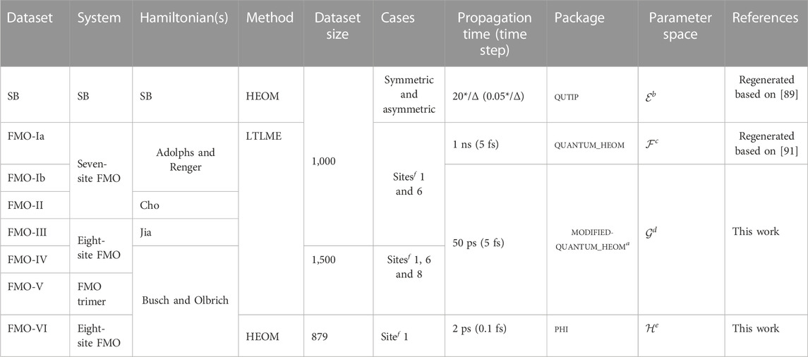
TABLE 1. Summary of all datasets. More details are given in the main text. Here, “SB” stands for the spin-boson model. ^amodified-quantum_HEOM is the quantum_HEOM package with some local modifications to make it compatible for larger Hamiltonians. ^bIn the parameter space $\mathcal{E}$, we define $\widetilde{ϵ}=ϵ/\mathrm{\Delta }=\{\mathrm{0,1}\}$, $\tilde{\lambda }=\lambda /\mathrm{\Delta }=\left\{0.1\right.$, 0.2, 0.3, 0.4, 0.5, 0.6, 0.7, 0.8, 0.9, 1.0}, $\tilde{\gamma }=\gamma /\mathrm{\Delta }=\left\{1\right.$, 2, 3, 4, 5, 6, 7, 8, 9, 10}, and $\tilde{\beta }=\beta \mathrm{\Delta }=\left\{0.1\right.$, 0.25, 0.5, 0.75, 1}, where the tunneling matrix element Δ is set as an energy unit. For all combinations of these parameters, the system reduced density matrix was propagated. ^cIn the parameter space $\mathcal{F}$, we choose the top 500 (most distant) combinations of (λ, γ, and T) based on farthest-point sampling. The parameter range for each dimension is λ = {10, 40, 70, …, 310} cm⁻¹; γ = {25, 50, 75, …, 300} fs rad⁻¹; and T = {30, 50, 70, …, 310} K. ^dIn the parameter space $\mathcal{G}$, we adopt the same procedure as in the parameter space $\mathcal{F}$ and choose the most distant 500 points (based on farthest-point sampling) from 3D space (λ, γ, and T) where λ = {10, 40, 70, …, 520} cm⁻¹; γ = {25, 50, 75, …, 500} cm⁻¹; and T = {30, 50, 70, …, 510} K. ^eIn the parameter space $\mathcal{H}$, the parameter range remains the same as in $\mathcal{G}$. In addition, the same farthest-point sampling was adopted but with the only difference being that instead of 500, 1,100 most distant sets of parameters were chosen. Approximately 20% of the initial dataset was removed because of the prohibitive memory requirements. For the remaining 80% of the dataset, HEOM calculations were performed for 2.0 ps using 0.1 fs as a time step. ^fIn the case of the FMO complex, this column lists the initially excited sites of the FMO complex in each subset of the corresponding dataset.

The FMO system has become one of the most extensively studied natural light-harvesting complexes [54–60]. Under physiological conditions, the FMO complex forms a homotrimer consisting of eight bacteriochlorophyll-a (BChla) molecules per monomer. The biological function of the FMO trimer is to transfer excitation energy from the chlorosome to the reaction center (RC) [61]. An interest in this light-harvesting system sparked when two-dimensional electronic spectroscopy experiments detected the presence of quantum coherence effects in the FMO complex [62]; [63]; [64]. These observations triggered intense debates about the role this coherence might play in highly efficient excitation energy transfer (EET).

Early studies of the FMO complex considered only seven-site FMO models comprising BChla 1–7. Until BChla 8 was discovered, BChla 1 and 6 were both assumed to be possible locations for accepting the excitation from the chlorosome because they are believed to be the nearest pigments to the antenna, which captures sunlight [65]; [66]; [67]. From there, the energy is subsequently funneled through two nearly independent routes: from site 1 to 2 (pathway 1) or from site 6 to sites 7, 5, and 4 (pathway 2). The terminal point of either route is site 3, where the exciton is then transferred to the RC [68].

Ever since the discovery of the eighth BChla, the role of this pigment in EET has been extensively investigated [69]; [70]; [71]; [72]; [58]; [73]; [74]; [68]; [75]. In particular, it was shown that while the population dynamics of the eight-site FMO model is markedly different from that of a seven-site configuration, the EET efficiencies in both models were predicted to remain comparable and very high [68]. BChla 8 has also been suggested as a possible recipient of the initial excitation.

The dynamics of the FMO model has been a subject of numerous computational studies, primarily focusing on understanding the role of the protein environment in the efficiency of EET (see, e.g., [76]; [77]; [78]; [79]). Numerical simulations typically employ one of the several parameterized or fitted into the experimental data FMO model Hamiltonians that differ in the BChla excitation energies and the couplings between different BChla [61]; [80]; [54]; [81]; [82]; [83]; [84]. Simulations of the full FMO trimer containing 24 BChlas have also been performed [85]; [86].

Accompanying this data report, the QD3SET-1 database contains seven datasets of time-evolved population dynamics of FMO models with different system Hamiltonians and initial excitations for several hundreds of bath and system–bath parameters. The hierarchy of equations of motion (HEOM) approach [5,7] was used to simulate the population dynamics of SB and FMO models, in one of the seven FMO datasets. HEOM is a numerically exact method that can describe the dynamics of a system with a non-perturbative and non-Markovian system–bath interaction. The high computational cost of HEOM, however, limits the number of FMO simulations that can be performed with this method. To generate the other six FMO datasets, an approximate method—the local thermalizing Lindblad master equation (LTLME) [87]; [88]—was used.

Some of our data were already used in previous studies developing and benchmarking ML models for quantum dynamics simulations [37,38]; [35]; [36]. Here, we regenerate one of the datasets to augment it with more data and provide many new datasets generated from scratch (Table 1). To facilitate their use, we organized the datasets in a coherently formatted database and provided metadata and extraction scripts. We expect that our database that accompanies this data report will serve as a valuable resource in the development of new quantum dynamics methods.

Methods

Spin-boson dataset

This dataset is regenerated with the same settings and parameters as in on our previous SB dataset [38] in order to include all the elements (populations and coherences) of the reduced density matrix (RDM) of the system. The populations and population differences were published and used previously [38]; [35]. In the following section, we provide a brief summary of the self-containing presentation of the dataset.

Spin-boson model

The spin-boson model comprises a two-level quantum subsystem (TLS) coupled to a bath of harmonic oscillators. The Hamiltonian has the following standard system–bath form: $\widehat{H}={\widehat{H}}_s+{\widehat{H}}_b+{\widehat{H}}_{sb}$. The Hamiltonian of the TLS in the local (or site) basis {| + ⟩, | − ⟩} is given by (ℏ = 1)

${\widehat{H}}_s=ϵ\left(|+\rangle \langle +|-|-\rangle \langle -|\right)+\mathrm{\Delta }\left(|+\rangle \langle -|+|-\rangle \langle +|\right),(1)$

where ϵ is the so-called energy bias and Δ is the tunneling matrix element. The harmonic bath is an ensemble of independent harmonic oscillators

${\widehat{H}}_b={\displaystyle \sum _{j=1}^{N_b}}\left(\frac{{\widehat{p}}_j^2}{2m_j}+\frac{1}{2}{m}_j{\omega }_j^2{\widehat{x}}_j^2\right),(2)$

where $\{{\widehat{x}}_j\}$ and $\{{\widehat{p}}_j\}$ are the coordinates and momenta, respectively, of N_b independent harmonic bath modes with masses {m_j} and frequencies {ω_j}. The TLS and bath are coupled through the additional term

${\widehat{H}}_{sb}=-{\displaystyle \sum _{j=1}^{N_b}}{c}_j{\widehat{x}}_j\left(|+\rangle \langle +|-|-\rangle \langle -|\right),(3)$

where {c_j} is the coupling coefficients.

The effects of the bath on the dynamics of the TLS are collectively determined by the spectral density function [89]

$J\left(\omega \right)=\frac{\pi }{2}{\displaystyle \sum _{j=1}^{N_b}}\frac{c_j^2}{m_j{\omega }_j}\delta \left(\omega -{\omega }_j\right).(4)$

In this work, we choose to employ the Debye form of the spectral density (Ohmic spectral density with the Drude–Lorentz cutoff) [90]

$J\left(\omega \right)=2\lambda \frac{\omega \gamma }{{\omega }^2+{\gamma }^2},(5)$

where λ is the bath reorganization energy, which controls the strength of system–bath coupling, and the cutoff frequency γ = 1/τ_c (τ_c is the bath relaxation time).

All dynamical properties of the TLS can be obtained from the RDM

${\tilde{\rho }}_{\alpha \beta }\left(t\right)={\text{Tr}}_b⟨\alpha |e^{-i\widehat{H}t/\hslash }\widehat{\rho }\left(0\right)e^{i\widehat{H}t/\hslash }|\beta ⟩,(6)$

where α, β ∈ {| + ⟩, | − ⟩}, $\widehat{\rho }$ is the total density operator, and the trace is taken over bath degrees of freedom. For example, the commonly used population difference in benchmark studies is obtained from the RDM as follows: $p_{+}(t)-p_{-}(t)={\tilde{\rho }}_{++}(t)-{\tilde{\rho }}_{--}(t)$.

The initial state of the total system is assumed to be a product state of the system and bath in the following form:

$\widehat{\rho }\left(0\right)={\widehat{\rho }}_{\text{s}}\left(0\right){\widehat{\rho }}_{\text{b}}\left(0\right).(7)$

In Eq. 7, the bath density operator is an equilibrium canonical density operator ${\widehat{\rho }}_b(0)=e^{-\beta {\widehat{H}}_{\text{b}}}/{\mathrm{Tr}}_{\text{b}}\left[e^{-\beta {\widehat{H}}_{\text{b}}}\right]$, where $\beta ={(k_{\text{B}}T)}^{-1}$ is the inverse temperature and k_B is the Boltzmann constant. The initial density operator of the system is chosen to be ${\widehat{\rho }}_{\text{s}}(0)=|+\rangle \langle +|$. These conditions correspond to instantaneous photoexcitation of the subsystem.

Data generation for the spin-boson model

The dataset for the spin-boson model was generated as described previously [38]. We also summarize it here. The following system and bath parameters were chosen: $\widetilde{ϵ}=ϵ/\mathrm{\Delta }=\{\mathrm{0,1}\}$, $\tilde{\lambda }=\lambda /\mathrm{\Delta }=\{0.1,0.2,0.3,0.4,0.5,0.6,0.7,0.8,0.9,1.0\}$, $\tilde{\gamma }=\gamma /\mathrm{\Delta }=\{\mathrm{1,2,3},\mathrm{4,5},\mathrm{6,7},\mathrm{8,9,10}\}$, and $\tilde{\beta }=\beta \mathrm{\Delta }=\{0.1,0.25,0.5,0.75,1\}$, where the tunneling matrix element Δ is set as an energy unit. For all combinations of these parameters, the system RDM was propagated using the HEOM approach implemented in the QuTiP software package [91]. The total propagation time was t_maxΔ = 20, and the HEOM integration time step was set to dtΔ = 0.05. In total, 1,000 HEOM calculations, 500 for symmetric (ϵ/Δ = 0) and 500 for asymmetric (ϵ/Δ = 1) spin-boson Hamiltonians, were performed. The dataset contains a set of RDMs from tΔ = 0 to t_maxΔ = 20, saved every dtΔ = 0.05, for every combination of the parameters $(\widetilde{ϵ},\tilde{\lambda },\tilde{\gamma },\tilde{\beta })$ described previously.

Fenna–Matthews–Olson complex datasets

In this section, we first describe the general theory behind the FMO model Hamiltonian, and later, for each dataset, we provide specific technical details. Table 1 provides an overview of each dataset.

FMO model Hamiltonian

The FMO complex in this work is described by the system–bath Hamiltonian with the renormalization term $\widehat{H}={\widehat{H}}_s+{\widehat{H}}_b+{\widehat{H}}_{sb}+{\widehat{H}}_{\mathit{ren}}$. The electronic system is described by the Frenkel exciton Hamiltonian

${\widehat{H}}_s={\displaystyle \sum _{n=1}^{N_e}}{E}_n|n\rangle \langle n|+{\displaystyle \sum _{n,m=1,n\ne m}^{N_e}}{V}_{nm}|n\rangle \langle m|,(8)$

where |n⟩ denotes that only the nth site is in its electronically excited state and all other sites are in their electronically ground states, E_n is the transition energies, and V_nm is the Coulomb coupling between nth and mth sites. The couplings are assumed to be constant (the Condon approximation). It should be noted that the overall electronic ground state of the pigment protein complex |0⟩ is assumed to be only radiatively coupled to the single-excitation manifold, and as such, it is not included in the dynamics calculations. Analogous with the SB model, the bath is modeled by a set of independent harmonic oscillators. The thermal bath is coupled to the subsystem’s states |n⟩ through the system–bath interaction term

${\widehat{H}}_{sb}={\displaystyle \sum _{n=1}^{N_e}}{\displaystyle \sum _{j=1}^{N_b}}{c}_{nj}{\widehat{x}}_j|n\rangle \langle n|,(9)$

where each subsystem’s state is independently coupled to its own harmonic environment and c_nj is the pigment–phonon coupling constants of environmental phonons local to the nth BChla.

The FMO model Hamiltonian contains a reorganization term that counters the shift in the minimum energy positions of harmonic oscillators introduced by the system–bath coupling. In the case that each state |n⟩ is independently coupled to the environment, the renormalization term takes the following form:

${\widehat{H}}_{\mathit{ren}}={\displaystyle \sum _{n=1}^{N_e}}{\lambda }_n|n\rangle \langle n|,(10)$

where ${\lambda }_n={\sum }_j{c}_{nj}^2/(2m_j{\omega }_j^2)$ is the bath reorganization energy. The bath spectral density associated with each electronic state is assumed to be given by the Lorentz–Drude spectral density (Eq. 5).

Analogous to the SB dataset, the initial state of the total system is assumed to be a product state of the system and bath. The initial electronic density operator given by ${\widehat{\rho }}_s(0)$ was varied, as described in the following section. The bath density operator is taken to be the equilibrium canonical density operator.

FMO-Ia, FMO-Ib, and FMO-II datasets: seven-site FMO models using the local thermalizing Lindblad master equation approach

We generated datasets for the two seven-site system (N_e = 7) Hamiltonians. The FMO-I dataset was generated for the system Hamiltonian parameterized by Adolphs and Renger [54], and is given by (in cm⁻¹)

$H_s=\left(\begin{array}{ccccccc}\hfill 200\hfill & \hfill -87.7\hfill & \hfill 5.5\hfill & \hfill -5.9\hfill & \hfill 6.7\hfill & \hfill -13.7\hfill & \hfill -9.9\hfill \\ \hfill -87.7\hfill & \hfill 320\hfill & \hfill 30.8\hfill & \hfill 8.2\hfill & \hfill 0.7\hfill & \hfill 11.8\hfill & \hfill 4.3\hfill \\ \hfill 5.5\hfill & \hfill 30.8\hfill & \hfill 0\hfill & \hfill -53.5\hfill & \hfill -2.2\hfill & \hfill -9.6\hfill & \hfill 6.0\hfill \\ \hfill -5.9\hfill & \hfill 8.2\hfill & \hfill -53.5\hfill & \hfill 110\hfill & \hfill -70.7\hfill & \hfill -17.0\hfill & \hfill -63.6\hfill \\ \hfill 6.7\hfill & \hfill 0.7\hfill & \hfill -2.2\hfill & \hfill -70.7\hfill & \hfill 270\hfill & \hfill 81.1\hfill & \hfill -1.3\hfill \\ \hfill -13.7\hfill & \hfill 11.8\hfill & \hfill -9.6\hfill & \hfill -17.0\hfill & \hfill 81.1\hfill & \hfill 420\hfill & \hfill 39.7\hfill \\ \hfill -9.9\hfill & \hfill 4.3\hfill & \hfill 6.0\hfill & \hfill -63.3\hfill & \hfill -1.3\hfill & \hfill 39.7\hfill & \hfill 230\hfill \end{array}\right).(11)$

The FMO-Ia dataset comes directly from our previous studies [37,49], and the FMO-Ib dataset was generated here for a broader parameter space described as follows.

The FMO-II dataset was generated for the Hamiltonian parameterized by Cho et al. [81], which takes the following form (in cm⁻¹):

$H_s=\left(\begin{array}{ccccccc}\hfill 280\hfill & \hfill -106\hfill & \hfill 8\hfill & \hfill -5\hfill & \hfill 6\hfill & \hfill -8\hfill & \hfill -4\hfill \\ \hfill -106\hfill & \hfill 420\hfill & \hfill 28\hfill & \hfill 6\hfill & \hfill 2\hfill & \hfill 13\hfill & \hfill 1\hfill \\ \hfill 8\hfill & \hfill 28\hfill & \hfill 0\hfill & \hfill -62\hfill & \hfill -1\hfill & \hfill -9\hfill & \hfill 17\hfill \\ \hfill -5\hfill & \hfill 6\hfill & \hfill -62\hfill & \hfill 175\hfill & \hfill -70\hfill & \hfill -19\hfill & \hfill -57\hfill \\ \hfill 6\hfill & \hfill 2\hfill & \hfill -1\hfill & \hfill -70\hfill & \hfill 320\hfill & \hfill 40\hfill & \hfill -2\hfill \\ \hfill -8\hfill & \hfill 13\hfill & \hfill -9\hfill & \hfill -19\hfill & \hfill 40\hfill & \hfill 360\hfill & \hfill 32\hfill \\ \hfill -4\hfill & \hfill 1\hfill & \hfill 17\hfill & \hfill -57\hfill & \hfill -2\hfill & \hfill 32\hfill & \hfill 260\hfill \end{array}\right).(12)$

The diagonal offset of 12,210 cm⁻¹ is added to both Hamiltonians. Each site is coupled to its own bath characterized by the Drude–Lorentz spectral density, Eq. 5, but the bath of each site is described by the same spectral density.

For the FMO-Ia dataset, the following spectral density parameters and temperatures were employed: λ = {10, 40, 70, …, 310} cm⁻¹; γ = {25, 50, 75, …, 300} fs rad⁻¹; and T = {30, 50, 70, …, 310} K. For the FMO-Ib and FMO-II datasets, the spectral density parameters and temperatures were λ = {10, 40, 70, …, 520} cm⁻¹; γ = {25, 50, 75, …, 500} cm⁻¹; and T = {30, 50, 70, …, 510} K. Our choice of temperatures is relevant for most of the experiments performed on the FMO and other photosynthetic complexes [92]; [93]; [56].

For FMO-Ia, FMO-Ib, and FMO-II datasets, farthest-point sampling [94] was employed to select the most distant points in the Euclidean space [37] of parameters, which typically more efficiently covers relevant space than random sampling [94]. We choose the top 500 (most distant) combinations of (λ, γ, and T) based on farthest-point sampling. For each selected set of parameters, the system RDM was calculated using the so-called local thermalizing Lindblad master equation (LTLME) approach [95]; [88]. Implemented in the quantum_HEOM package [5,96], the LTLME method is based on the Lindblad quantum master equation, which is the commonly used approach to study the dynamics of open quantum systems [97]; [98]; [99]. Specifically, in the LTLME approach, for each unique frequency gap between eigenstates of the system Hamiltonian and for every possible combination of site n, Lindblad operators are constructed. A sum is carried out over all transitions with a unique frequency, and the contribution of each population transfer is weighted by $c_n^{*}({\mathrm{\Omega }}^{\prime })c_n(\mathrm{\Omega })$, where c_n(Ω) is the nth site coefficient of exciton (eigenstate) Ω, while $c_n^{*}({\mathrm{\Omega }}^{\prime })$ is the complex conjugate corresponding to exciton Ω′. More details can be found in the work of Mohseni et al. [95].

Coming to data generation, two subsets of the dataset were generated, one for the initial electronic density operator ${\widehat{\rho }}_s(0)=|1\rangle \langle 1|$ corresponding to the initial excitation of site 1 and the other one for the initial density operator ${\widehat{\rho }}_s(0)=|6\rangle \langle 6|$ corresponding to the initial excitation of site 6. In each case, 500 RDM trajectories were generated. The dataset contains both diagonal (populations) and off-diagonal (coherences) elements of the RDM on a time grid from 0 to 1 ns (in the case of FMO-Ia) and 0 to 50 ps (in the case of FMO-Ib and FMO-II) with a 5 fs time step.

FMO-III and FMO-IV datasets: eight-site FMO models using the local thermalizing Lindblad master equation approach

Using the same LTLME-based approach, we generated a dataset for two different Hamiltonians for the eight-site FMO model. The first Hamiltonian (FMO-III dataset) was parameterized by Jia et al. [75]. The electronic system Hamiltonian is given by (in cm⁻¹)

$H_s=\left(\begin{array}{cccccccc}\hfill 218\hfill & \hfill -91.0\hfill & \hfill 4.1\hfill & \hfill -6.3\hfill & \hfill 6.3\hfill & \hfill -8.8\hfill & \hfill -7.8\hfill & \hfill 32.4\hfill \\ \hfill -91.0\hfill & \hfill 81\hfill & \hfill 28.7\hfill & \hfill 8.2\hfill & \hfill 1.0\hfill & \hfill 8.8\hfill & \hfill 3.4\hfill & \hfill 6.3\hfill \\ \hfill 4.1\hfill & \hfill 28.7\hfill & \hfill 0\hfill & \hfill -46.6\hfill & \hfill -4.4\hfill & \hfill -9.3\hfill & \hfill 1.3\hfill & \hfill 1.3\hfill \\ \hfill -6.3\hfill & \hfill 8.2\hfill & \hfill -46.6\hfill & \hfill 105\hfill & \hfill -73.9\hfill & \hfill -17.7\hfill & \hfill -59.1\hfill & \hfill -1.9\hfill \\ \hfill 6.3\hfill & \hfill 1.0\hfill & \hfill -4.4\hfill & \hfill -73.9\hfill & \hfill 105\hfill & \hfill 76.0\hfill & \hfill -3.1\hfill & \hfill 4.2\hfill \\ \hfill -8.8\hfill & \hfill 8.8\hfill & \hfill -9.3\hfill & \hfill -17.7\hfill & \hfill 76.0\hfill & \hfill 186\hfill & \hfill 25.9\hfill & \hfill -11.6\hfill \\ \hfill -7.8\hfill & \hfill 3.4\hfill & \hfill 1.3\hfill & \hfill -59.1\hfill & \hfill -3.1\hfill & \hfill 25.9\hfill & \hfill 169\hfill & \hfill -11.9\hfill \\ \hfill 32.4\hfill & \hfill 6.3\hfill & \hfill 1.3\hfill & \hfill -1.9\hfill & \hfill 4.2\hfill & \hfill -11.6\hfill & \hfill -11.9\hfill & \hfill 154\hfill \end{array}\right),(13)$

with a diagonal offset of 11,332 cm⁻¹.

The FMO-IV dataset was generated for the Hamiltonian parameterized by Busch et al. [69] (site energies) and Olbrich et al. [72] (excitonic couplings) and takes the following form (in cm⁻¹):

$H_s=\left(\begin{array}{cccccccc}\hfill 310\hfill & \hfill -80.3\hfill & \hfill 3.5\hfill & \hfill -4.0\hfill & \hfill 4.5\hfill & \hfill -10.2\hfill & \hfill -4.9\hfill & \hfill 21.0\hfill \\ \hfill -80.3\hfill & \hfill 230\hfill & \hfill 23.5\hfill & \hfill 6.7\hfill & \hfill 0.5\hfill & \hfill 7.5\hfill & \hfill 1.5\hfill & \hfill 3.3\hfill \\ \hfill 3.5\hfill & \hfill 23.5\hfill & \hfill 0\hfill & \hfill -49.8\hfill & \hfill -1.5\hfill & \hfill -6.5\hfill & \hfill 1.2\hfill & \hfill 0.7\hfill \\ \hfill -4.0\hfill & \hfill 6.7\hfill & \hfill -49.8\hfill & \hfill 180\hfill & \hfill 63.4\hfill & \hfill -13.3\hfill & \hfill -42.2\hfill & \hfill -1.2\hfill \\ \hfill 4.5\hfill & \hfill 0.5\hfill & \hfill -1.5\hfill & \hfill 63.4\hfill & \hfill 450\hfill & \hfill 55.8\hfill & \hfill 4.7\hfill & \hfill 2.8\hfill \\ \hfill -10.2\hfill & \hfill 7.5\hfill & \hfill -6.5\hfill & \hfill -13.3\hfill & \hfill 55.8\hfill & \hfill 320\hfill & \hfill 33.0\hfill & \hfill -7.3\hfill \\ \hfill -4.9\hfill & \hfill 1.5\hfill & \hfill 1.2\hfill & \hfill -42.2\hfill & \hfill 4.7\hfill & \hfill 33.0\hfill & \hfill 270\hfill & \hfill -8.7\hfill \\ \hfill 21.0\hfill & \hfill 3.3\hfill & \hfill 0.7\hfill & \hfill -1.2\hfill & \hfill 2.8\hfill & \hfill -7.3\hfill & \hfill -8.7\hfill & \hfill 505\hfill \end{array}\right),(14)$

with a diagonal offset of 12,195 cm⁻¹.

The same set of spectral density parameters and temperatures that was used in the generation of the FMO-Ib and FMO-II datasets was used here. The LTLME method was used to propagate the system RDM from 0 to 50 ps with a 5 fs time step, and three initial states of the electronic system were considered: sites 1, 6, and 8. The dataset contains both diagonal (populations) and off-diagonal (coherences) elements of the RDM. The calculations were performed using the quantum_HEOM package [96] with some local modifications to make it compatible for the Hamiltonians with larger dimension. We refer to this as modified-quantum_HEOM implementation.

FMO-V dataset: FMO trimer using the local thermalizing Lindblad master equation approach

Additionally, we also generated a dataset for the FMO trimer. The overall excitonic Hamiltonian of all three subunits is given by

$H_s=\left(\begin{array}{ccc}\hfill H_A\hfill & \hfill H_B\hfill & \hfill H_B^T\hfill \\ \hfill H_B^T\hfill & \hfill H_A\hfill & \hfill H_B\hfill \\ \hfill H_B\hfill & \hfill H_B^T\hfill & \hfill H_A\hfill \end{array}\right),(15)$

where H_A is the subunit Hamiltonian for which we used the same Hamiltonian as in the FMO-IV dataset (Eq. 14), while H_B is the inter-subunit Hamiltonian, which is taken from the work of Olbrich et al. [72] and is given by (in cm⁻¹)

$H_B=\left(\begin{array}{cccccccc}\hfill 1.0\hfill & \hfill 0.3\hfill & \hfill -0.6\hfill & \hfill 0.7\hfill & \hfill 2.3\hfill & \hfill 1.5\hfill & \hfill 0.9\hfill & \hfill 0.1\hfill \\ \hfill 1.5\hfill & \hfill -0.4\hfill & \hfill -2.5\hfill & \hfill -1.5\hfill & \hfill 7.4\hfill & \hfill 5.2\hfill & \hfill 1.5\hfill & \hfill 0.7\hfill \\ \hfill 1.4\hfill & \hfill 0.1\hfill & \hfill -2.7\hfill & \hfill 5.7\hfill & \hfill 4.6\hfill & \hfill 2.3\hfill & \hfill 4.0\hfill & \hfill 0.8\hfill \\ \hfill 0.3\hfill & \hfill 0.5\hfill & \hfill 0.7\hfill & \hfill 1.9\hfill & \hfill -0.6\hfill & \hfill -0.4\hfill & \hfill 1.9\hfill & \hfill -0.8\hfill \\ \hfill 0.7\hfill & \hfill 0.9\hfill & \hfill 1.1\hfill & \hfill -0.1\hfill & \hfill 1.8\hfill & \hfill 0.1\hfill & \hfill -0.7\hfill & \hfill 1.3\hfill \\ \hfill 0.1\hfill & \hfill 0.7\hfill & \hfill 0.8\hfill & \hfill 1.4\hfill & \hfill -1.4\hfill & \hfill -1.5\hfill & \hfill 1.6\hfill & \hfill -1.0\hfill \\ \hfill 0.3\hfill & \hfill 0.2\hfill & \hfill -0.7\hfill & \hfill 4.8\hfill & \hfill -1.6\hfill & \hfill 0.1\hfill & \hfill 5.7\hfill & \hfill -2.3\hfill \\ \hfill 0.1\hfill & \hfill 0.6\hfill & \hfill 1.5\hfill & \hfill -1.1\hfill & \hfill 4.0\hfill & \hfill -3.1\hfill & \hfill -5.2\hfill & \hfill 3.6\hfill \end{array}\right).(16)$

We propagate dynamics with LTLME from 0 to 50 ps with a 5 fs time step for the same parameters as were adopted in the calculations for the FMO-Ib–FMO-IV datasets. The calculations were performed with the modified-quantum_HEOM implementation for the initial excited sites 1, 6, and 8.

FMO-VI dataset: an eight-site FMO model using the hierarchy of equations of motion approach

The LTLME approach provides only an approximate description of the quantum dynamics of the FMO complex. Therefore, the FMO-I–FMO-V datasets are useful merely for developing machine learning models for quantum dynamics studies. For example, they can be used to train a neural network model, which can then be further improved on more accurate but smaller datasets (e.g., via transfer learning). However, LTLME dynamics cannot be used to benchmark other quantum dynamics methods. In this case, high-quality reference data are needed.

To generate a dataset with accurate FMO dynamics, we performed HEOM calculations for the eight-site FMO model with the Hamiltonian given by Eq. 14. HEOM calculations were performed using the parallel hierarchy integrator (PHI) code [100]. The initial dataset was chosen on the basis of farthest-point sampling, similar to how it was performed in the FMO-Ib–FMO-V datasets, with the only difference being that instead of the 500 most distant sets of parameters that were chosen in the preparation of FMO-Ib–FMO-V data sets, the 1,100 most distant sets of parameters were used to prepare the initial FMO-VI dataset. For certain parameters, the RAM requirements exceeded the RAM of computing nodes available to us (1 TB). Therefore, such parameter sets were excluded from the dataset. Excluded parameters correspond to low temperatures, high reorganization energies, and low cutoff frequencies. Such strong non-Markovian regimes pose significant challenges in the computational studies of open quantum systems. Approximately 20% of the initial dataset was removed because of prohibitive memory requirements. We note that even though graphics processing unit (GPU) implementations of HEOM (e.g., Kreisbeck et al. [101]) are much faster than their CPU-based counterparts, they are still limited by the small amount of memory in presently available GPUs.

For the remaining 80% of the dataset, HEOM calculations were performed for 2.0 ps. To speed up calculations, an adaptive integration Runge–Kutta–Fehlberg 4/5 [102] (RKF45) method was used, as implemented in the PHI code. Using adaptive integration reduces both the total computation time and memory requirements but can lead to artifacts if the accuracy threshold is set too large [100]. In this work, the PHI default accuracy threshold of 1·10⁻⁶ was used. The initial integration time step was set to 0.1 fs. In RKF45, the integration time step is varied, and therefore, the output comprises time-evolved RDMs on an unevenly spaced time grid. To obtain the RDMs on an evenly spaced time grid of 0.1 fs, cubic spline interpolation was used. The interpolation errors were examined on a few cases where 0.1 fs fixed time step integration was feasible. The errors in the populations were found to be less than 10⁻⁵, which is much smaller than the convergence thresholds, as illustrated in the Technical Validation section of Supplementary Material. The final FMO-VI dataset contains 879 entries, each comprising all the populations and coherences for the RDM from 0 to 2 ps with a time step of 0.1 fs.

In Figure 1, we present a comparison of the dynamics of the eight-site FMO model described by Eq. 14. The calculations were performed using the LTLME and HEOM methods for two different parameter sets: T = 330 K, λ = 10 cm⁻¹, and γ = 475 cm⁻¹ and T = 310 K, λ = 430 cm⁻¹, and γ = 75 cm⁻¹. The results clearly demonstrate the differences between the two methods. HEOM, being a numerically exact method, accurately captures the coherence dynamics of the FMO Hamiltonian. On the other hand, LTLME is an approximate method that does not fully account for the back-reaction from the bath to the system. As a result, it tends to underestimate the coherence dynamics in this context.

FIGURE 1

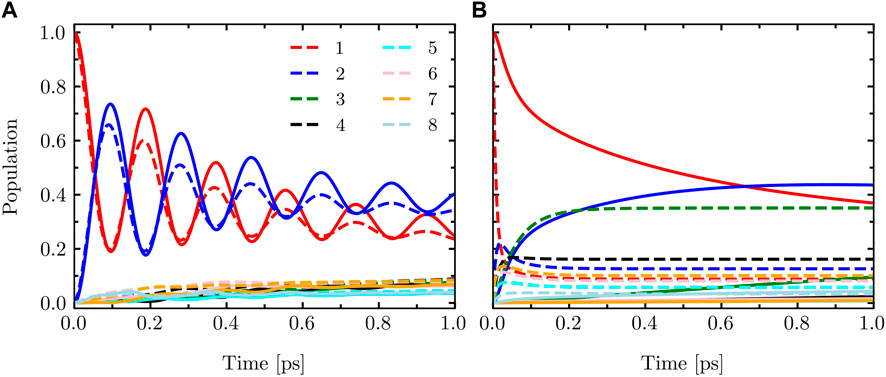
FIGURE 1. Population dynamics of the eight-site FMO model with the system Hamiltonian given by Eq. 14 calculated using HEOM (solid) and LTLME (dashed) methods for the following parameters (A): T = 330 K, λ = 10 cm⁻¹, and γ = 475 cm⁻¹ and (B) T = 310 K, λ = 430 cm⁻¹, and γ = 75 cm⁻¹.

Data availability statement

All data sets can be accessed at Figshare https://doi.org/10.25452/figshare.plus.c.6389553. The data sets are stored in standard NumPy [103] binary file format (.npy) files. The following format of file names was adopted in the SB data set 2_epsilon-X_Delta-1.0_lambda-Y_gamma-Z_beta-XX.npy where X denotes the value of the energy bias (∼ε), Y is the reorganization energy ∼λ, Z is the cut-off frequency ∼γ and XX is the inverse temperature ∼β. The following format of file names was adopted in all FMO data sets X_initial-Y_gamma-Z_lambda-XX_temp-YY.npy, where X denotes the number of sites in the FMO model, Y is the initial state, Z is the value of bath frequency, XX is the value of reorganization energy, and YY is the temperature. A Python package for extracting data is provided together with the data set and can be accessed at https://github.com/Arif-PhyChem/QD3SET.

Author contributions

PD and AU conceived the idea of creating a HEOM-based spin-boson database. AU conceived the idea of creating an LTLME-based database for the FMO complex. AK conceived the idea of creating an FMO dataset using the HEOM method. AU performed the HEOM calculations for the spin-boson, along with the LTLME calculations for the FMO complex. AU wrote the provided package for easy extraction of the data. AK and LH performed the calculations and created database files for the FMO-VI dataset. All authors analyzed the results. AK took the lead in writing the original draft of the manuscript. All authors contributed to the article and approved the submitted version.

Funding

This work was supported by General University Research (GUR) Grants and startup funds of the College of Arts and Sciences and the Department of Physics and Astronomy of the University of Delaware. PD acknowledges funding by the National Natural Science Foundation of China [No. 22003051 and funding via the Outstanding Youth Scholars (Overseas, 2021) project], the Fundamental Research Funds for the Central Universities (No. 20720210092), and via the Lab project of the State Key Laboratory of Physical Chemistry of Solid Surfaces. This project was supported by the Science and Technology Projects of Innovation Laboratory for Sciences and Technologies of Energy Materials of Fujian Province (IKKEM) (No. RD2022070103). AK acknowledges the Ralph E. Powe Junior Faculty Enhancement Award from Oak Ridge Associated Universities.

Acknowledgments

This research was supported in part through the use of Data Science Institute (DSI) computational resources at the University of Delaware. Calculations were also performed with high-performance computing resources provided by the Xiamen University.

Conflict of interest

The authors declare that the research was conducted in the absence of any commercial or financial relationships that could be construed as a potential conflict of interest.

Publisher’s note

All claims expressed in this article are solely those of the authors and do not necessarily represent those of their affiliated organizations, or those of the publisher, the editors, and the reviewers. Any product that may be evaluated in this article, or claim that may be made by its manufacturer, is not guaranteed or endorsed by the publisher.

Supplementary material

The Supplementary Material for this article can be found online at: https://www.frontiersin.org/articles/10.3389/fphy.2023.1223973/full#supplementary-material

References

1. Meyer H, Gatti F, Worth G. Multidimensional quantum dynamics: MCTDH theory and applications. Wiley (2009).

Google Scholar

2. Makri N. Time-dependent quantum methods for large systems. Annu Rev Phys Chem (1999) 50:167–91. doi:10.1146/annurev.physchem.50.1.167

PubMed Abstract | CrossRef Full Text | Google Scholar

3. Meyer H-D, Manthe U, Cederbaum L. The multi-configurational time-dependent Hartree approach. Chem Phys Lett (1990) 165:73–8. doi:10.1016/0009-2614(90)87014-I

CrossRef Full Text | Google Scholar

4. Wang H, Thoss M. Multilayer formulation of the multiconfiguration time-dependent hartree theory. J Chem Phys (2003) 119:1289–99. doi:10.1063/1.1580111

CrossRef Full Text | Google Scholar

5. Tanimura Y. Numerically “exact” approach to open quantum dynamics: The hierarchical equations of motion (HEOM). J Chem Phys (2020) 153:020901. doi:10.1063/5.0011599

PubMed Abstract | CrossRef Full Text | Google Scholar

6. Tanimura Y, Kubo R. Two-time correlation functions of a system coupled to a heat bath with a Gaussian–Markoffian interaction. Proc Jpn Soc (1989) 58:1199–206. doi:10.1143/jpsj.58.1199

CrossRef Full Text | Google Scholar

7. Tanimura Y. Nonperturbative expansion method for a quantum system coupled to a harmonic-oscillator bath. Phys Rev A (1990) 41:6676–87. doi:10.1103/PhysRevA.41.6676

PubMed Abstract | CrossRef Full Text | Google Scholar

8. Greene SM, Batista VS. Tensor-train split-operator Fourier transform (tt-soft) method: Multidimensional nonadiabatic quantum dynamics. J Chem Theor Comput. (2017) 13:4034–42. doi:10.1021/acs.jctc.7b00608

CrossRef Full Text | Google Scholar

9. Kapral R. Progress in the theory of mixed quantum-classical dynamics. Annu Rev Phys Chem (2006) 57:129–57. doi:10.1146/annurev.physchem.57.032905.104702

PubMed Abstract | CrossRef Full Text | Google Scholar

10. Kapral R. Surface hopping from the perspective of quantum–classical Liouville dynamics. Chem Phys (2016) 481:77–83. doi:10.1016/j.chemphys.2016.05.016

CrossRef Full Text | Google Scholar

11. Min SK, Agostini F, Tavernelli I, Gross EK. Ab initio nonadiabatic dynamics with coupled trajectories: A rigorous approach to quantum (de) coherence. J Phys Chem Lett (2017) 8:3048–55. doi:10.1021/acs.jpclett.7b01249

PubMed Abstract | CrossRef Full Text | Google Scholar

12. Min SK, Agostini F, Gross EKU. Coupled-Trajectory quantum-classical approach to electronic decoherence in nonadiabatic processes. Phys Rev Lett (2015) 115:073001. doi:10.1103/physrevlett.115.073001

PubMed Abstract | CrossRef Full Text | Google Scholar

13. Gao X, Geva E. Improving the accuracy of quasiclassical mapping Hamiltonian methods by treating the window function width as an adjustable parameter. The J Phys Chem A (2020) 124:11006–16. doi:10.1021/acs.jpca.0c09750

PubMed Abstract | CrossRef Full Text | Google Scholar

14. Crespo-Otero R, Barbatti M. Recent advances and perspectives on nonadiabatic mixed quantum–classical dynamics. Chem Rev (2018) 118:7026–68. doi:10.1021/acs.chemrev.7b00577

PubMed Abstract | CrossRef Full Text | Google Scholar

15. Subotnik JE, Jain A, Landry B, Petit A, Ouyang W, Bellonzi N. Understanding the surface hopping view of electronic transitions and decoherence. Annu Rev Phys Chem (2016) 67:387–417. doi:10.1146/annurev-physchem-040215-112245

PubMed Abstract | CrossRef Full Text | Google Scholar

16. Wang L, Akimov A, Prezhdo OV. Recent progress in surface hopping: 2011–2015. J Phys Chem Lett (2016) 7:2100–12. doi:10.1021/acs.jpclett.6b00710

PubMed Abstract | CrossRef Full Text | Google Scholar

17. McLachlan AD. A variational solution of the time-dependent Schrodinger equation. Mol Phys (2006) 8:39–44. doi:10.1080/00268976400100041

CrossRef Full Text | Google Scholar

18. Tully JC. Molecular dynamics with electronic transitions. J Chem Phys (1990) 93:1061–71. doi:10.1063/1.459170

CrossRef Full Text | Google Scholar

19. Shushkov P, Li R, Tully JC. Ring polymer molecular dynamics with surface hopping. J Chem Phys (2012) 137:22A549. doi:10.1063/1.4766449

PubMed Abstract | CrossRef Full Text | Google Scholar

20. Huo P, Miller TF, Coker DF. Communication: Predictive partial linearized path integral simulation of condensed phase electron transfer dynamics. J Chem Phys (2013) 139:151103. doi:10.1063/1.4826163

PubMed Abstract | CrossRef Full Text | Google Scholar

21. Kapral R, Ciccotti G. Mixed quantum-classical dynamics. J Chem Phys (1999) 110:8919–29. doi:10.1063/1.478811

CrossRef Full Text | Google Scholar

22. Miller WH, Cotton SJ. Classical molecular dynamics simulation of electronically non-adiabatic processes. Faraday Discuss (2016) 195:9–30. doi:10.1039/c6fd00181e

PubMed Abstract | CrossRef Full Text | Google Scholar

23. Sun X, Geva E. Equilibrium fermi’s golden rule charge transfer rate constants in the condensed phase: The linearized semiclassical method vs classical marcus theory. J Phys Chem A (2016) 120:2976–90. doi:10.1021/acs.jpca.5b08280

PubMed Abstract | CrossRef Full Text | Google Scholar

24. Chenu A, Scholes GD. Coherence in energy transfer and photosynthesis. Annu Rev Phys Chem (2015) 66:69–96. doi:10.1146/annurev-physchem-040214-121713

PubMed Abstract | CrossRef Full Text | Google Scholar

25. Han L, Ullah A, Yan Y-A, Zheng X, Yan Y, Chernyak V. Stochastic equation of motion approach to fermionic dissipative dynamics. i. formalism. J Chem Phys (2020) 152:204105. doi:10.1063/1.5142164

PubMed Abstract | CrossRef Full Text | Google Scholar

26. Ullah A, Han L, Yan Y-A, Zheng X, Yan Y, Chernyak V. Stochastic equation of motion approach to fermionic dissipative dynamics. ii. numerical implementation. J Chem Phys (2020) 152:204106. doi:10.1063/1.5142166

PubMed Abstract | CrossRef Full Text | Google Scholar

27. Yan Y-A, Zheng X, Shao J. Piecewise ensemble averaging stochastic liouville equations for simulating non-markovian quantum dynamics. New J Phys (2022) 24:103012. doi:10.1088/1367-2630/ac94f1

CrossRef Full Text | Google Scholar

28. Chen Z-H, Wang Y, Zheng X, Xu R-X, Yan Y. Universal time-domain prony fitting decomposition for optimized hierarchical quantum master equations. J Chem Phys (2022) 156:221102. doi:10.1063/5.0095961

PubMed Abstract | CrossRef Full Text | Google Scholar

29. Runeson JE, Lawrence JE, Mannouch JR, Richardson JO. Explaining the efficiency of photosynthesis: Quantum uncertainty or classical vibrations? J Phys Chem Lett (2022) 13:3392–9. doi:10.1021/acs.jpclett.2c00538

PubMed Abstract | CrossRef Full Text | Google Scholar

30. Runeson JE, Richardson JO. Generalized spin mapping for quantum-classical dynamics. J Chem Phys (2020) 152:084110. doi:10.1063/1.5143412

PubMed Abstract | CrossRef Full Text | Google Scholar

31. Guo M, Wang Z, Wang F. Equation-of-motion coupled-cluster theory for double electron attachment with spin–orbit coupling. J Chem Phys (2020) 153:214118. doi:10.1063/5.0032716

PubMed Abstract | CrossRef Full Text | Google Scholar

32. Mandal A, Yamijala SS, Huo P. Quasi-diabatic representation for nonadiabatic dynamics propagation. J Chem Theor Comput (2018) 14:1828–40. doi:10.1021/acs.jctc.7b01178

CrossRef Full Text | Google Scholar

33. Ye J, Sun K, Zhao Y, Yu Y, Kong Lee C, Cao J. Excitonic energy transfer in light-harvesting complexes in purple bacteria. J Chem Phys (2012) 136:245104. doi:10.1063/1.4729786

PubMed Abstract | CrossRef Full Text | Google Scholar

34. Herrera Rodríguez LE, Kananenka AA. Convolutional neural networks for long time dissipative quantum dynamics. J Phys Chem Lett (2021) 12:2476–83. doi:10.1021/acs.jpclett.1c00079

PubMed Abstract | CrossRef Full Text | Google Scholar

35. Herrera LE, Ullah A, Rueda KJ, Dral PO, Kananenka A. A comparative study of different machine learning methods for dissipative quantum dynamics. Machine Learn Sci Tech (2022) 3:045016. doi:10.1088/2632-2153/ac9a9d

CrossRef Full Text | Google Scholar

36. Ullah A, Dral PO. One-shot trajectory learning of open quantum systems dynamics. J Phys Chem Lett (2022) 13:6037–41. doi:10.1021/acs.jpclett.2c01242

PubMed Abstract | CrossRef Full Text | Google Scholar

37. Ullah A, Dral PO. Predicting the future of excitation energy transfer in light-harvesting complex with artificial intelligence-based quantum dynamics. Nat Commun (2022) 13:1930–8. doi:10.1038/s41467-022-29621-w

PubMed Abstract | CrossRef Full Text | Google Scholar

38. Ullah A, Dral PO. Speeding up quantum dissipative dynamics of open systems with kernel methods. New J Phys (2021) 23:113019. doi:10.1088/1367-2630/ac3261

CrossRef Full Text | Google Scholar

39. Naicker K, Sinayskiy I, Petruccione F. Machine learning for excitation energy transfer dynamics. Phys Rev Res (2022) 4:033175. doi:10.1103/physrevresearch.4.033175

CrossRef Full Text | Google Scholar

40. Akimov AV. Extending the time scales of nonadiabatic molecular dynamics via machine learning in the time domain. J Phys Chem Lett (2021) 12:12119–28. doi:10.1021/acs.jpclett.1c03823

PubMed Abstract | CrossRef Full Text | Google Scholar

41. Secor M, Soudackov AV, Hammes-Schiffer S. Artificial neural networks as propagators in quantum dynamics. J Phys Chem Lett (2021) 12:10654–62. doi:10.1021/acs.jpclett.1c03117

PubMed Abstract | CrossRef Full Text | Google Scholar

42. Banchi L, Grant E, Rocchetto A, Severini S. Modelling non-markovian quantum processes with recurrent neural networks. New J Phys (2018) 20:123030. doi:10.1088/1367-2630/aaf749

CrossRef Full Text | Google Scholar

43. Bandyopadhyay S, Huang Z, Sun K, Zhao Y. Applications of neural networks to the simulation of dynamics of open quantum systems. Chem Phys (2018) 515:272–8. doi:10.1016/j.chemphys.2018.05.019

CrossRef Full Text | Google Scholar

44. Yang B, He B, Wan J, Kubal S, Zhao Y. Applications of neural networks to dynamics simulation of Landau–Zener transitions. Chem Phys (2020) 528:110509. doi:10.1016/j.chemphys.2019.110509

CrossRef Full Text | Google Scholar

45. Wu D, Hu Z, Li J, Sun X. Forecasting nonadiabatic dynamics using hybrid convolutional neural network/long short-term memory network. J Chem Phys (2021) 155:224104. doi:10.1063/5.0073689

PubMed Abstract | CrossRef Full Text | Google Scholar

46. Lin K, Peng J, Gu FL, Lan Z. Simulation of open quantum dynamics with bootstrap-based long short-term memory recurrent neural network. J Phys Chem Lett (2021) 12:10225–34. doi:10.1021/acs.jpclett.1c02672

PubMed Abstract | CrossRef Full Text | Google Scholar

47. Tang D, Jia L, Shen L, Fang WH. Fewest-switches surface hopping with long short-term memory networks. J Phys Chem Lett (2022) 13:10377–87. doi:10.1021/acs.jpclett.2c02299

PubMed Abstract | CrossRef Full Text | Google Scholar

48. Lin K, Peng J, Xu C, Gu FL, Lan Z. Realization of the trajectory propagation in the mm-sqc dynamics by using machine learning (2022). arXiv preprint arXiv:2207.05556.

Google Scholar

49. Lin K, Peng J, Xu C, Gu FL, Lan Z. Automatic evolution of machine-learning-based quantum dynamics with uncertainty analysis. J Chem Theor Comput (2022) 18:5837–55. doi:10.1021/acs.jctc.2c00702

CrossRef Full Text | Google Scholar

50. Choi M, Flam-Shepherd D, Kyaw TH, Aspuru-Guzik A. Learning quantum dynamics with latent neural ordinary differential equations. Phys Rev A (2022) 105:042403. doi:10.1103/PhysRevA.105.042403

CrossRef Full Text | Google Scholar

51. Zhang L, Ullah A, Pinheiro M, Dral PO, Barbatti M. Excited-state dynamics with machine learning. In: Quantum Chemistry in the age of machine learning. Elsevier (2023). p. 329–53.

CrossRef Full Text | Google Scholar

52. Leggett AJ, Chakravarty S, Dorsey AT, Fisher MPA, Garg A, Zwerger W. Dynamics of the dissipative two-state system. Rev Mod Phys (1987) 59:1–85. doi:10.1103/revmodphys.59.1

CrossRef Full Text | Google Scholar

53. Weiss U. Quantum Dissipative Systems. Series in modern condensed matter physics. World Scientific (2012).

Google Scholar

54. Adolphs J, Renger T. How proteins trigger excitation energy transfer in the fmo complex of green sulfur bacteria. Biophys J (2006) 91:2778–97. doi:10.1529/biophysj.105.079483

PubMed Abstract | CrossRef Full Text | Google Scholar

55. Ishizaki A, Fleming GR. Theoretical examination of quantum coherence in a photosynthetic system at physiological temperature. Proc Natl Acad Sci U.S.A (2009) 106:17255–60. doi:10.1073/pnas.0908989106

PubMed Abstract | CrossRef Full Text | Google Scholar

56. Panitchayangkoon G, Hayes D, Fransted KA, Caram JR, Harel E, Wen J, et al. Long-lived quantum coherence in photosynthetic complexes at physiological temperature. Proc Natl Acad Sci U.S.A (2010) 107:12766–70. doi:10.1073/pnas.1005484107

PubMed Abstract | CrossRef Full Text | Google Scholar

57. Harush EZ, Dubi Y. Do photosynthetic complexes use quantum coherence to increase their efficiency? Probably not. Sci Adv (2021) 7:eabc4631. doi:10.1126/sciadv.abc4631

PubMed Abstract | CrossRef Full Text | Google Scholar

58. Ritschel G, Roden J, Strunz WT, Aspuru-Guzik A, Eisfeld A. Absence of quantum oscillations and dependence on site energies in electronic excitation transfer in the Fenna–Matthews–Olson trimer. J Phys Chem Lett (2011) 2:2912–7. doi:10.1021/jz201119j

CrossRef Full Text | Google Scholar

59. Shim S, Rebentrost P, Valleau S, Aspuru-Guzik A. Atomistic study of the long-lived quantum coherences in the Fenna–Matthews–Olson complex. Biophys J (2012) 102:649–60. doi:10.1016/j.bpj.2011.12.021

PubMed Abstract | CrossRef Full Text | Google Scholar

60. Fenna RE, Matthews BW. Chlorophyll arrangement in a bacteriochlorophyll protein from Chlorobium limicola. Nature (1975) 258:573–7. doi:10.1038/258573a0

CrossRef Full Text | Google Scholar

61. Milder MTW, Brüggemann B, Grondelle RV, Herek JL. Revisiting the optical properties of the FMO protein. Photosynthesis Res (2010) 104:257–74. doi:10.1007/s11120-010-9540-1

PubMed Abstract | CrossRef Full Text | Google Scholar

62. Engel GS, Calhoun TR, Read EL, Ahn T-K, Mancal T, Cheng YC, et al. Evidence for wavelike energy transfer through quantum coherence in photosynthetic systems. Nature (2007) 446:782–6. doi:10.1038/nature05678

PubMed Abstract | CrossRef Full Text | Google Scholar

63. Scholes GD, Fleming GR, Chen LX, Aspuru-Guzik A, Buchleitner A, Coker DF, et al. Using coherence to enhance function in chemical and biophysical systems. Nature (2017) 543:647–56. doi:10.1038/nature21425

PubMed Abstract | CrossRef Full Text | Google Scholar

64. Engel GS. Quantum coherence in photosynthesis. Proced Chem (2011) 3:222–31. 22nd Solvay Conference on Chemistry. doi:10.1016/j.proche.2011.08.029

CrossRef Full Text | Google Scholar

65. Renger T, May V. Ultrafast exciton motion in photosynthetic antenna systems: The fmo-complex. J Phys Chem A (1998) 102:4381–91. doi:10.1021/jp9800665

CrossRef Full Text | Google Scholar

66. Louwe RJW, Vrieze J, Hoff AJ, Aartsma TJ. Toward an integral interpretation of the optical steady-state spectra of the fmo-complex of prosthecochloris aestuarii. 2. exciton simulations. The J Phys Chem B (1997) 101:11280–7. doi:10.1021/jp9722162

CrossRef Full Text | Google Scholar

67. List NH, Curutchet C, Knecht S, Mennucci B, Kongsted J. Toward reliable prediction of the energy ladder in multichromophoric systems: A benchmark study on the fmo light-harvesting complex. J Chem Theor Comput (2013) 9:4928–38. doi:10.1021/ct400560m

CrossRef Full Text | Google Scholar

68. Moix J, Wu J, Huo P, Coker D, Cao J. Efficient energy transfer in light-harvesting systems, III: The influence of the eighth bacteriochlorophyll on the dynamics and efficiency in FMO. J Phys Chem Lett (2011) 2:3045–52. doi:10.1021/jz201259v

CrossRef Full Text | Google Scholar

69. Busch MSa., Mü h F, Madjet ME-A, Renger T. The eighth bacteriochlorophyll completes the excitation energy funnel in the FMO protein. J Phys Chem Lett (2011) 2:93–8. doi:10.1021/jz101541b

PubMed Abstract | CrossRef Full Text | Google Scholar

70. Huang RY-C, Wen J, Blankenship RE, Gross ML. Hydrogen–deuterium exchange mass spectrometry reveals the interaction of fenna–matthews–olson protein and chlorosome csma protein. Biochemistry (2012) 51:187–93. doi:10.1021/bi201620y

PubMed Abstract | CrossRef Full Text | Google Scholar

71. Bina D, Blankenship RE. Chemical oxidation of the FMO antenna protein from Chlorobaculum tepidum. Photosynthesis Res (2013) 116:11–9. doi:10.1007/s11120-013-9878-2

PubMed Abstract | CrossRef Full Text | Google Scholar

72. Olbrich C, Jansen TLC, Liebers J, Aghtar M, Strumpfer J, Schulten K, et al. From atomistic modeling to excitation transfer and two-dimensional spectra of the FMO light-harvesting complex. J Phys Chem B (2011) 115:8609–21. doi:10.1021/jp202619a

PubMed Abstract | CrossRef Full Text | Google Scholar

73. Mühlbacher L, Kleinekathöfer U. Preparational effects on the excitation energy transfer in the fmo complex. J Phys Chem B (2012) 116:3900–6. doi:10.1021/jp301444q

PubMed Abstract | CrossRef Full Text | Google Scholar

74. Tronrud DE, Wen J, Gay L, Blankenship RE. The structural basis for the difference in absorbance spectra for the FMO antenna protein from various green sulfur bacteria. Photosynthesis Res (2009) 100:79–87. doi:10.1007/s11120-009-9430-6

PubMed Abstract | CrossRef Full Text | Google Scholar

75. Jia X, Mei Y, Zhang JZ, Mo Y. Hybrid QM/MM study of FMO complex with polarized protein-specific charge. Scientific Rep (2015) 5:17096. doi:10.1038/srep17096

PubMed Abstract | CrossRef Full Text | Google Scholar

76. Shabani A, Mohseni M, Rabitz H, Lloyd S. Efficient estimation of energy transfer efficiency in light-harvesting complexes. Phys Rev E (2012) 86:011915. doi:10.1103/PhysRevE.86.011915

PubMed Abstract | CrossRef Full Text | Google Scholar

77. Wu J, Liu F, Shen Y, Cao J, Silbey RJ. Efficient energy transfer in light-harvesting systems, i: Optimal temperature, reorganization energy and spatial–temporal correlations. New J Phys (2010) 12:105012. doi:10.1088/1367-2630/12/10/105012

CrossRef Full Text | Google Scholar

78. Suzuki Y, Watanabe H, Okiyama Y, Ebina K, Tanaka S. Comparative study on model parameter evaluations for the energy transfer dynamics in Fenna–Matthews–Olson complex. Chem Phys (2020) 539:110903. doi:10.1016/j.chemphys.2020.110903

CrossRef Full Text | Google Scholar

79. Mohseni M, Shabani A, Lloyd S, Rabitz H. Energy-scales convergence for optimal and robust quantum transport in photosynthetic complexes. J Chem Phys (2014) 140:035102. doi:10.1063/1.4856795

PubMed Abstract | CrossRef Full Text | Google Scholar

80. Vulto SIE, Baat MAD, Louwe RJW, Permentier HP, Neef T, Miller M, et al. Exciton simulations of optical spectra of the FMO complex from the green sulfur bacterium chlorobium tepidum at 6 K. J Phys Chem B (1998) 102:9577–82. doi:10.1021/jp982095l

CrossRef Full Text | Google Scholar

81. Cho M, Vaswani HM, Brixner T, Stenger J, Fleming GR. Exciton analysis in 2D electronic spectroscopy. J Phys Chem B (2005) 109:10542–56. doi:10.1021/jp050788d

PubMed Abstract | CrossRef Full Text | Google Scholar

82. Hayes D, Engel G. Extracting the excitonic Hamiltonian of the fenna-matthews-olson complex using three-dimensional third-order electronic spectroscopy. Biophysical J (2011) 100:2043–52. doi:10.1016/j.bpj.2010.12.3747

PubMed Abstract | CrossRef Full Text | Google Scholar

83. Kell A, Blankenship RE, Jankowiak R. Effect of spectral density shapes on the excitonic structure and dynamics of the fenna–matthews–olson trimer from chlorobaculum tepidum. J Phys Chem A (2016) 120:6146–54. doi:10.1021/acs.jpca.6b03107

PubMed Abstract | CrossRef Full Text | Google Scholar

84. Rolczynski BS, Yeh S-H, Navotnaya P, Lloyd LT, Ginzburg AR, Zheng H, et al. Time-domain line-shape analysis from 2d spectroscopy to precisely determine Hamiltonian parameters for a photosynthetic complex. J Phys Chem B (2021) 125:2812–20. doi:10.1021/acs.jpcb.0c08012

PubMed Abstract | CrossRef Full Text | Google Scholar

85. Ke Y, Zhao Y. Hierarchy of forward-backward stochastic Schrödinger equation. J Chem Phys (2016) 145:024101. doi:10.1063/1.4955107

PubMed Abstract | CrossRef Full Text | Google Scholar

86. Wilkins DM, Dattani NS. Why quantum coherence is not important in the fenna–matthews–olsen complex. J Chem Theor Comput (2015) 11:3411–9. doi:10.1021/ct501066k

CrossRef Full Text | Google Scholar

87. Bourne Worster S, Stross C, Vaughan FM, Linden N, Manby FR. Structure and efficiency in bacterial photosynthetic light harvesting. J Phys Chem Lett (2019) 10:7383–90. doi:10.1021/acs.jpclett.9b02625

PubMed Abstract | CrossRef Full Text | Google Scholar

88. Abbott JW. Quantum dynamics of bath influenced excitonic energy transfer in photosynthetic pigment-protein complexes. Master Thesis. Bristol: University of Bristol United Kingdom (2020). doi:10.5281/zenodo.7229807

CrossRef Full Text | Google Scholar

89. Caldeira A, Leggett A. Path integral approach to quantum Brownian motion. Physica A: Stat Mech its Appl (1983) 121:587–616. doi:10.1016/0378-4371(83)90013-4

CrossRef Full Text | Google Scholar

90. Wang H, Song X, Chandler D, Miller WH. Semiclassical study of electronically nonadiabatic dynamics in the condensed-phase: Spin-boson problem with debye spectral density. J Chem Phys (1999) 110:4828–40. doi:10.1063/1.478388

CrossRef Full Text | Google Scholar

91. Johansson J, Nation P, Nori F. Qutip: An open-source python framework for the dynamics of open quantum systems. Comput Phys Commun (2012) 183:1760–72. doi:10.1016/j.cpc.2012.02.021

CrossRef Full Text | Google Scholar

92. Brixner T, Stenger J, Vaswani HM, Cho M, Blankenship RE, Fleming GR. Two-dimensional spectroscopy of electronic couplings in photosynthesis. Nature (2005) 434:625–8. doi:10.1038/nature03429

PubMed Abstract | CrossRef Full Text | Google Scholar

93. Harel E, Engel GS. Quantum coherence spectroscopy reveals complex dynamics in bacterial light-harvesting complex 2 (LH2). Proc Natl Acad Sci (2012) 109:706–11. doi:10.1073/pnas.1110312109

PubMed Abstract | CrossRef Full Text | Google Scholar

94. Dral PO. Mlatom: A program package for quantum chemical research assisted by machine learning. J Comput Chem (2019) 40:2339–47. doi:10.1002/jcc.26004

PubMed Abstract | CrossRef Full Text | Google Scholar

95. Mohseni M, Rebentrost P, Lloyd S, Aspuru-Guzik A. Environment-assisted quantum walks in photosynthetic energy transfer. J Chem Phys (2008) 129:174106. doi:10.1063/1.3002335

PubMed Abstract | CrossRef Full Text | Google Scholar

96. Abbott JW. jwa7/quantum_heom (2019). Github repository: https://github.com/jwa7/quantum_HEOM (accessed on November 1, 2022).

Google Scholar

97. Breuer H-P, Petruccione F. The theory of open quantum systems. New York, NY: Oxford University Press (2002).

Google Scholar

98. Gardiner C, Zoller P, Zoller P. Quantum noise: A handbook of markovian and non-markovian quantum stochastic methods with applications to quantum optics. In: Springer series in synergetics. Springer (2004).

Google Scholar

99. Rivas Á, Huelga S. SpringerBriefs in physics. Springer Berlin Heidelberg (2011).Open quantum systems: An introduction

Google Scholar

100. Strümpfer J, Schulten K. Open quantum dynamics calculations with the hierarchy equations of motion on parallel computers. J Chem Theor Comput (2012) 8:2808–16. doi:10.1021/ct3003833

CrossRef Full Text | Google Scholar

101. Kreisbeck C, Kramer T, Rodríguez M, Hein B. High-performance solution of hierarchical equations of motion for studying energy transfer in light-harvesting complexes. J Chem Theor Comput (2011) 7:2166–74. doi:10.1021/ct200126d

CrossRef Full Text | Google Scholar

102. Fehlberg E. Some old and new Runge-Kutta formulas with stepsize control and their error coefficients. Computing (1985) 34:265–70. doi:10.1007/bf02253322

CrossRef Full Text | Google Scholar

103. Oliphant TE. Python for scientific computing. Comput Sci Eng (2007) 9:10–20. doi:10.1109/mcse.2007.58

CrossRef Full Text | Google Scholar