Adaptive command-filtered finite-time consensus tracking control for single-link flexible-joint robotic multi-agent systems

This article presents a command-filtered finite-time consensus tracking control strategy for the considered single-link flexible-joint robotic multi-agent systems. First, each agent system considered in this article is a nonlinear nonstrict-feedback system with unknown nonlinearities, so the traditional backstepping method cannot be directly applied to the design controller. However, by applying the unique structure of the Gaussian function in radial basis function neural networks, the challenges in controller design caused by the aforementioned nonstrict-feedback system have been overcome. Second, the problem of unknown nonlinearities in the system is solved by the approximation property of radial basis function neural network technology. In addition, the traditional backstepping approach often leads to an “explosion of complexity” resulting from repeated derivation of virtual control signals. Our design addresses this issue by employing command filtering technology, which simplifies the controller design process. Meanwhile, new compensation signals are designed, which successfully eliminate the error influence posed by the filters. It is seen that the control strategy presented in this article can guarantee the tracking errors converge to a small neighborhood of origin in a finite time, and all signals in the closed-loop systems remain bounded. Eventually, the simulation results show the validity of the acquired control scheme.

1 Introduction

As industrial automation continues to evolve, the study of flexible-joint robots has become increasingly popular. Recently, numerous control strategies have been proposed for research on robots with flexible joints [1–6]. For example, in [7], a prescribed performance tracking control approach was introduced for free-flying flexible-joint space robots that experience disturbances due to input saturation. Meanwhile, in [8], a full-state tracking control approach was proposed for the flexible-joint robots with singular perturbation techniques. However, the aforementioned flexible-joint robot system is a single system, which cannot meet the needs of practical engineering in the age of network communication. At present, the study of the consensus tracking control of multi-agent systems (MASs) has also received widespread attention [9–12]. For instance, an event-triggered coordination via a Lyapunov-based approach was presented for MASs in [9]. Compared with the single system, MASs have higher pragmatic value in the industrial field, such as the formation of unmanned aerial vehicles, autonomous underwater vehicles, and intelligent robot cooperation. Nevertheless, there are relatively few studies on single-link flexible-joint robotic MASs due to the complex structure of such systems and the influence of frequent information interaction.

Significantly, the study of nonlinear systems is a hot topic at present [13–18], and most practical systems are unknown nonlinear systems, which will bring great difficulties to the controller design. Accordingly, fuzzy logic systems (FLSs) were applied to deal with unknown nonlinearities in the system due to their excellent universal approximation performance [19–22]. For example, an adaptive fuzzy control method was proposed for nontriangular structure nonlinear systems in the study by Li et al. [23]. In [24,25], FLSs were further introduced to handle the unknown nonlinearities of robot systems. However, the aforementioned proposed methods are not applicable for nonlinear nonstrict-feedback systems. By comparison, neural network (NN) technology not only has excellent approximation performance [26–30] but also can deal with the difficulties of the controller design for nonstrict-feedback systems. Therefore, in [31], the radial basis function neural network (RBF NN) technology was introduced to handle unknown nonlinearities in nonstrict-feedback systems, and the simulation proved the validity of the approximation ability of the RBF NN technology. It is worth noting that the aforementioned research studies always had the challenge of “explosion of complexity,” which can add to the complexity of the controller design process. Lately, several research studies have proposed the dynamic surface control (DSC) technology by utilizing first-order filters to tackle the challenge of “explosion of complexity” in the controller design process [32–34]. For instance, in [35], an adaptive fuzzy decentralized DSC approach was presented for switched large-scale nonlinear systems with full-state constraints. Nevertheless, the boundary layer errors generated by the filters are difficult to be handled using the DSC technique. Therefore, the command filtering technology was applied to uncertain switched nonlinear systems, which simultaneously settled the problem of “explosion of complexity” and the influence of boundary layer errors in [36]. It is noteworthy that the disadvantages of the DSC technology are overcome by designing the error compensation signals in using the command filtering technology. However, practical systems have very high requirements for the convergence speed of systems, but the control methods proposed earlier cannot ensure system stability in finite time. Therefore, how to devise a finite-time control strategy for the considered system is an extremely significant research topic.

Considering the practical industrial application, the finite-time tracking control is very significant, which can ensure that the system states converge to the equilibrium point in finite time. The finite-time stability was defined for the equilibrium point of continuous but non-Lipschitzian autonomous systems in [37], which was widely used in the design procedure of the finite-time controller. Based on this theory, the research on the finite-time control problem has made great progress. For instance, in order to address full-state constrained nonlinear systems with dead zone, researchers combined the adaptive backstepping method with barrier Lyapunov functions, ultimately presenting the adaptive finite-time tracking control approach as outlined in [38]. By proposing the finite-time control schemes, in [39], the control method of nonlinear systems with actuator failures was investigated. In addition, in [40], a finite-time command-filtered backstepping method was designed to solve finite-time control issues for systems with input saturation. Nevertheless, the finite-time control strategies proposed earlier cannot be directly applied to single-link flexible-joint robotic MASs with nonstrict-feedback and the directed communication topology.

In view of the aforestated discussions, a new adaptive command-filtered finite-time consensus tracking control strategy is presented for the considered single-link flexible-joint robotic MASs, which solves the difficulties caused by nonstrict-feedback and “explosion of complexity.” The characteristics of this article are given as follows: (1) In contrast to the previous research in [36,41], the considered MASs in this paper are nonlinear nonstrict-feedback systems, which are more extensively applied in actual application than nonlinear strict-feedback systems. (2) Different from the conventional backstepping method in [28], the presented command-filtered control strategy in this article overcomes the challenge of “explosion of complexity” so that the complexity of the controller design procedure is simplified. Meanwhile, new compensation signals are devised in the command filter technology, which eliminate the error effect caused by the filters. (3) In [42], the proposed control strategy for nonlinear MASs with flexible-joint manipulators can reach stability only when time tends to infinity. Therefore, the finite-time control strategy is designed for the considered nonlinear nonstrict-feedback single-link flexible-joint robotic MASs in this paper for the first time, which can guarantee that the tracking errors converge to a small neighborhood of origin and that all the closed-loop systems are stable within a finite time.

2 Problem statement and preliminaries

2.1 Graph theory

In this paper, we consider N agents and the directed topology graph among the agents, which can be described as G = (V, E). V = {1, …, N} represents the set of nodes. E ⊆ V × V represents the set of edges. An edge can be described as e_ji = (j, i) ∈ E, which expresses that agent i can get the information from agent j. Meanwhile, agent j is described as the neighbor of agent i. Then, the neighbor set of agent i is represented by N_i = {j|(j, i) ∈ E}. Furthermore, the adjacency matrix is defined as A = [a_ij] ∈ R^N×N. The element a_ij > 0 if e_ji = (j, i) ∈ E; otherwise, a_ij = 0. Generally, self-edge (i, i) is not allowed, which means that the diagonal elements of A are all zeros, i.e., a_ii = 0. Next, we define an in-degree matrix D = diag{d₁, d₂, …, d_N} ∈ R^N×N as a diagonal matrix, and its diagonal elements are $d_i={\sum }_{j=1}^N{a}_{ij}$for agent i. Hence, the Laplacian matrix of digraph G can be expressed as L = D − A.

The augmented graph $\bar{G}$ can be described as the corresponding topology between the leader and the followers generally when the leader is considered. Therefore, $\bar{G}=(\bar{V},\bar{E})$ represents the augmented graph. $\bar{V}$ represents the node sets, including the leader and the followers. $\bar{E}$represents the edge sets, displaying the communication relationship between the leader and the followers. The diagonal elements b_i > 0 of B = diag{b_i} ∈ R^N×N denote that there is a weight between agent i and the leader, which is b_i = 0 otherwise. If a directed graph has a directed path from the root to every other node, it is said to have a spanning tree.

2.2 Problem statement

We consider a nonlinear flexible-joint robotic MAS with a leader and N followers. The dynamics of agent i in Figure 1 are given as follows:

$\left\{\begin{array}{c}{J}_1{\ddot{q}}_{i,1}+F_1{\dot{q}}_{i,1}+K\left(q_{i,1}-\frac{q_{i,2}}{N}\right)+Mgd\cos q_{i,1}=0,\hfill \\ J_2{\ddot{q}}_{i,2}+F_2{\dot{q}}_{i,2}-\frac{K}{N}\left(q_{i,1}-\frac{q_{i,2}}{N}\right)=K_t{I}_i,\hfill \\ L\dot{I_i}+R{I}_i+K_b{\dot{q}}_{i,2}=u_i,\hfill \end{array}\right.(1)$

where q_i,1, ${\dot{q}}_{i,1}$, and ${\ddot{q}}_{i,1}$ represent the link position, velocity, and acceleration, respectively. q_i,2, ${\dot{q}}_{i,2}$, and ${\ddot{q}}_{i,2}$ denote the motor shaft position, velocity, and acceleration, respectively. I_i denotes the armature current. J₁ and J₂ represent the link inertias. F₁ and F₂ are the viscous friction constants. K, K_t, and K_b denote the spring constant, torque constant, and back-emf constant, respectively. M, g, d, N, L, and R are the link mass, acceleration of gravity, position of the link center of gravity, gear ratio, armature inductance, and armature resistance, respectively. u_i is the armature voltage.

FIGURE 1

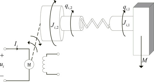
FIGURE 1. The single-link flexible-joint robotic manipulator of agent i.

For the convenience of studying system (1), we define x_i,1 = q_i,1, $x_{i,2}={\dot{q}}_{i,1}$, x_i,3 = q_i,2, $x_{i,4}={\dot{q}}_{i,2}$, and x_i,5 = I_i. Then, system (1) can be transformed as follows:

$\left\{\begin{array}{c}{\dot{x}}_{i,1}=x_{i,2},\hfill \\ {\dot{x}}_{i,2}={\delta }_{i,2}\left(x_{i,1},x_{i,2},x_{i,3}\right)+x_{i,3},\hfill \\ {\dot{x}}_{i,3}=x_{i,4},\hfill \\ {\dot{x}}_{i,4}={\delta }_{i,4}\left(x_{i,1},x_{i,2},x_{i,3},x_{i,4},x_{i,5}\right)+x_{i,5},\hfill \\ {\dot{x}}_{i,5}={\delta }_{i,5}\left(x_{i,1},x_{i,2},x_{i,3},x_{i,4},x_{i,5}\right)+\frac{1}{L}{u}_i,\hfill \\ y_i=x_{i,1},\hfill \end{array}\right.(2)$

where ${\delta }_{i,2}(x_{i,1},x_{i,2},x_{i,3})={J_1}^{-1}(-Mgd\cos x_{i,1}-F_1{x}_{i,2}-K(x_{i,1}-\frac{x_{i,3}}{N})-x_{i,3})$xi,3), ${\delta }_{i,4}(x_{i,1},x_{i,2},x_{i,3},x_{i,4},x_{i,5})={J_2}^{-1}(\frac{K}{N}(x_{i,1}-\frac{x_{i,3}}{N})-F_2{x}_{i,4}+K_t{x}_{i,5}-x_{i,5})$, δ_i,5(x_i,1, x_i,2, x_i,3, x_i,4, x_i,5) = L⁻¹(−Rx_i,5 − K_bx_i,4), and $x_i={\left[x_{i,1},\cdots x_{i,5}\right]}^T\in R^5$ are the whole states of agent i. y_i and u_i represent the output and control input of agent i, respectively. To simplify the design procedure of the controller, the parameters of the functions will be omitted in the subsequent design procedure. For example, the function δ_i,2(x_i,1, x_i,2, x_i,3) is expressed as δ_i,2. After that, the dynamic model of the leader is expressed as

$\begin{array}{c}{\dot{x}}_d=f_d\left(x_d,t\right),\hfill \\ y_d=x_d,\hfill \end{array}(3)$

where y_d ∈ R means the output of the leader. f_d(x_d, t) is a piecewise continuous function, which meets the local Lipschitz condition about x_d for t ≥ 0.

Assumption 1. In the augmented graph $\bar{G}$, the leader is the root node of a directed spanning tree. Additionally, each agent i can only receive state information from its neighbors.

Assumption 2. There is a continuous function f(⋅) and a positive constant X_d, which makes the inequalities $\left|f_d(x_d,t)\right|\le f(x_d)$ and $\left|x_d(t)\right|\le X_d$ hold for all t ≥ t₀.

2.3 Preliminaries

Our goal is to present an adaptive consensus tracking control protocol for the flexible-joint robotic MASs (2) to make sure that the tracking errors converge to a small neighborhood of origin within a finite time and that all signals in the closed-loop systems remain bounded. Therefore, the following knowledge is needed in the design process of the controller:

Lemma 1. (See [43]). For ∀ψ ∈ R, the following inequality is true:

$0\le \left|\psi \right|-\psi \tanh \left(\frac{\psi }{t}\right)\le \rho t,\forall t\ge 0,(4)$

where ρ = 0.2785.

Lemma 2. (See [44]). For any variable, ι, γ, one has

${\left|\iota \right|}^{{\kappa }_1}{\left|\gamma \right|}^{{\kappa }_2}\le \frac{{\kappa }_1}{{\kappa }_1+{\kappa }_2}{\kappa }_3{\left|\iota \right|}^{{\kappa }_1+{\kappa }_2}+\frac{{\kappa }_2}{{\kappa }_1+{\kappa }_2}{\kappa }_3^{-\frac{{\kappa }_1}{{\kappa }_2}}{\left|\gamma \right|}^{{\kappa }_1+{\kappa }_2},(5)$

where κ₁, κ₂, and κ₃ are arbitrary positive constants.

Lemma 3. (See [45]). For s_i ∈ R, i = 1, 2, …, n, and 0 < j ≤ 1, it holds that

${\left({\displaystyle \sum _{i=1}^n}\left|s_i\right|\right)}^j\le {\displaystyle \sum _{i=1}^n}{\left|s_i\right|}^j\le n^{1-j}{\left({\displaystyle \sum _{i=1}^n}\left|s_i\right|\right)}^j.(6)$

Definition 1. (See [41]). For any incipient condition ζ(0) ∈ ζ₀, if there is a constant ɛ > 0 and a settling time T(ɛ, ζ₀) < ∞ such that

$‖\zeta \left(t\right)‖<\epsilon ,\forall t>T,(7)$

the solution, which belongs to the nonlinear system $\dot{\zeta }=f(\zeta (t))$, is practical finite-time stable.

Lemma 4. (See [46]). The solution of $\dot{\zeta }=f(\zeta (t))$ is practical finite-time stable if there is a positive-definite function that meets the following formula:

$\dot{V}\left(\zeta \right)\le -\alpha V\left(\zeta \right)-\beta V^p\left(\zeta \right)+\mathrm{\Gamma },(8)$

where the design constants α > 0, β > 0, 0 < p < 1, and 0 < Γ < ∞.

RBF NNs [47]: In this paper, RBF NN technology is utilized to approximate unknown continuous functions. For the unknown continuous nonlinear function h(Z): R^S → R defined over a compact set Ω_Z ∈ R^s and the given precision ɛ* > 0, h(Z) can be approximated by RBF NNs as follows:

$h\left(Z\right)={\theta }^{*T}\phi \left(Z\right)+\epsilon \left(Z\right),(9)$

where Z ∈ Ω_Z ⊂ R^s is the input vector. ɛ(Z) denotes the approximation error with $\left|\epsilon (Z)\right|\le {\epsilon }^{*}$. $\phi (Z)={[{\phi }_1(Z),\dots ,{\phi }_l(Z)]}^T$ represents the basis function vector, and l > 1 represents a positive integer. Generally, the basis function φ_i(Z) can been chosen as the following Gaussian function:

${\phi }_i\left(Z\right)=\exp \left[-\frac{{\left(Z-{\mu }_i\right)}^T\left(Z-{\mu }_i\right)}{{{\kappa }_i}^2}\right],i=1,\dots ,l,(10)$

where ${\mu }_i={[{\mu }_{i1},\dots ,{\mu }_{il}]}^T$ and κ_i are the center and the width of the Gaussian function, respectively. In addition, ${\theta }^{*}={[{\theta }_1,\dots ,{\theta }_l]}^T\in R^l$ represents an ideal weight vector defined as

${\theta }^{*}=\arg \underset{\theta \in R^l}{\min }\left\{\underset{Z\in {\mathrm{\Omega }}_Z}{\sup }\left|h\left(Z\right)-{\theta }^T\phi \left(Z\right)\right|\right\},(11)$

where θ is the weight vector.

Lemma 5. (See [31]). Suppose $h({\bar{x}}_q)={[h_1({\bar{x}}_q),\dots ,h_l({\bar{x}}_q)]}^T$ is the basis function vector of RBF NNs, where ${\bar{x}}_q={[x_1,\dots ,x_q]}^T$. Then, the following inequality holds:

${‖h\left({\bar{x}}_q\right)‖}^2\le {‖h\left({\bar{x}}_L\right)‖}^2,(12)$

where the arbitrary positive integer L satisfies L ≤ q.

3 Controller design and stability analysis

3.1 Controller design

In this section, we design an adaptive command-filtered finite-time consensus tracking control scheme for MASs (2). The consensus tracking error of agent i is defined as

$z_{i,1}={\displaystyle \sum _{j=1}^N}{a}_{ij}\left(y_i-y_j\right)+b_i\left(y_i-y_d\right),(13)$

where a_ij and b_i are defined in the graph theory.

Remark 1. It is worth noting that (13) includes a_ij and b_i. Therefore, the consensus tracking error z_i,1 is influenced by the topology structure of the augmented graph $\bar{G}$. Furthermore, b_i + d_i > 0 is met for all the agents.

The coordinate transformation is designed as follows:

$z_{i,k}=x_{i,k}-{\bar{\alpha }}_{i,k},(14)$

where k = 2, …, 5. ${\bar{\alpha }}_{i,k}$ represents the output of the following command filter:

${\tau }_{i,k}{\dot{\stackrel{̄}{\alpha }}}_{i,k}+{\bar{\alpha }}_{i,k}={\alpha }_{i,k},{\bar{\alpha }}_{i,k}\left(0\right)={\alpha }_{i,k}\left(0\right),(15)$

where τ_i,k > 0 is a design constant. α_i,k is both the input of the command filter and the virtual controller, which will be presented later. Then, considering the impact of the error brought by the command filter (15), we define the following compensating signals:

$\left\{\begin{array}{c}{\dot{\eta }}_{i,1}=-\left(c_{i,1}+1\right){\eta }_{i,1}+\left(d_i+b_i\right){\eta }_{i,2}+\left(d_i+b_i\right)\left({\bar{\alpha }}_{i,2}-{\alpha }_{i,2}\right)-{\lambda }_{i,1}\mathrm{sgn}\left({\eta }_{i,1}\right),\hfill \\ {\dot{\eta }}_{i,2}=-\left(c_{i,2}+1\right){\eta }_{i,2}+{\eta }_{i,3}+\left({\bar{\alpha }}_{i,3}-{\alpha }_{i,3}\right)-\left(d_i+b_i\right){\eta }_{i,1}-{\lambda }_{i,2}\mathrm{sgn}\left({\eta }_{i,2}\right),\hfill \\ {\dot{\eta }}_{i,3}=-\left(c_{i,3}+\frac{1}{2}\right){\eta }_{i,3}+{\eta }_{i,4}+\left({\bar{\alpha }}_{i,4}-{\alpha }_{i,4}\right)-{\eta }_{i,2}-{\lambda }_{i,3}\mathrm{sgn}\left({\eta }_{i,3}\right),\hfill \\ {\dot{\eta }}_{i,4}=-\left(c_{i,4}+1\right){\eta }_{i,4}+{\eta }_{i,5}+\left({\bar{\alpha }}_{i,5}-{\alpha }_{i,5}\right)-{\eta }_{i,3}-{\lambda }_{i,4}\mathrm{sgn}\left({\eta }_{i,4}\right),\hfill \\ {\dot{\eta }}_{i,5}=-\left(c_{i,5}+1\right){\eta }_{i,5}-{\eta }_{i,4}-{\lambda }_{i,5}\mathrm{sgn}\left({\eta }_{i,5}\right),\hfill \end{array}\right.(16)$

where c_i,k > 0, λ_i,k > 0, and η_i,k(0) = 0 for k = 1, 2, 3, 4, 5. Next, we define the compensated tracking error v_i,k = z_i,k − η_i,k for k = 1, 2, 3, 4, 5.

Then, the virtual controllers are designed as follows:

$\left\{\begin{array}{c}{\alpha }_{i,2}=\frac{1}{d_i+b_i}\left(-\left(c_{i,1}+1\right)z_{i,1}-e_{i,1}{v}_{i,1}^{2p-1}-\frac{1}{2a_{i,1}^2}{v}_{i,1}{\widehat{\theta }}_{i,1}{\phi }_{i,1}^T{\phi }_{i,1}\right),\hfill \\ {\alpha }_{i,3}=-\left(c_{i,2}+1\right)z_{i,2}-e_{i,2}{v}_{i,2}^{2p-1}-\frac{1}{2a_{i,2}^2}{v}_{i,2}{\widehat{\theta }}_{i,2}{\phi }_{i,2}^T{\phi }_{i,2}-\left(d_i+b_i\right)z_{i,1}+{\dot{\stackrel{̄}{\alpha }}}_{i,2},\hfill \\ {\alpha }_{i,4}=-\left(c_{i,3}+\frac{1}{2}\right)z_{i,3}-e_{i,3}{v}_{i,3}^{2p-1}-z_{i,2}+{\dot{\stackrel{̄}{\alpha }}}_{i,3},\hfill \\ {\alpha }_{i,5}=-\left(c_{i,4}+1\right)z_{i,4}-e_{i,4}{v}_{i,4}^{2p-1}-\frac{1}{2a_{i,4}^2}{v}_{i,4}{\widehat{\theta }}_{i,4}{\phi }_{i,4}^T{\phi }_{i,4}-z_{i,3}+{\dot{\stackrel{̄}{\alpha }}}_{i,4},\hfill \end{array}\right.(17)$

where 1/2 < p < 1, p = ϖ₁/ϖ₂ and ϖ₁, ϖ₂ are odd integers. ${\widehat{\theta }}_{i,k}$ denotes the estimation of θ_i,k, and the estimation error is ${\tilde{\theta }}_{i,k}={\theta }_{i,k}-{\widehat{\theta }}_{i,k}$. e_i,k and a_i,k are positive design parameters.

Consequently, the adaptive laws are designed as follows:

${\dot{\widehat{\theta }}}_{i,k}=\frac{r_{i,k}}{2a_{i,k}^2}{v}_{i,k}^2{\phi }_{i,k}^T{\phi }_{i,k}-{\sigma }_{i,k}{\widehat{\theta }}_{i,k},(18)$

where r_i,k and σ_i,k are positive design parameters for k = 1, 2, 4, 5.

Then, we give the detailed design process for the system controllers.

Step 1. Taking the derivative of v_i,1, one has

$\begin{array}{c}\hfill \begin{array}{cc}\hfill {\dot{v}}_{i,1}& ={\dot{z}}_{i,1}-{\dot{\eta }}_{i,1}\hfill \\ \hfill & ={\displaystyle \sum _{j=1}^N}{a}_{i,j}\left({\dot{y}}_i-{\dot{y}}_j\right)+b_i\left({\dot{y}}_i-{\dot{y}}_d\right)-{\dot{\eta }}_{i,1}\hfill \\ \hfill & ={\displaystyle \sum _{j=1}^N}{a}_{i,j}\left(x_{i,2}-x_{j,2}\right)+b_i\left(x_{i,2}-f_d\left(x_d,t\right)\right)-{\dot{\eta }}_{i,1}\hfill \\ \hfill & =\left(d_i+b_i\right)x_{i,2}-b_i{f}_d\left(x_d,t\right)-{\displaystyle \sum _{j=1}^N}{a}_{i,j}{x}_{j,2}-{\dot{\eta }}_{i,1}.\hfill \end{array}\hfill \end{array}(19)$

Then, we design the following candidate Lyapunov function:

$V_{i,1}=\frac{1}{2}{v}_{i,1}^2+\frac{1}{2r_{i,1}}{\tilde{\theta }}_{i,1}^2.(20)$

Next, the derivation of V_i,1 is given as follows:

$\begin{array}{c}\hfill \begin{array}{cc}\hfill {\dot{V}}_{i,1}& =v_{i,1}{\dot{v}}_{i,1}-\frac{1}{r_{i,1}}{\tilde{\theta }}_{i,1}{\dot{\widehat{\theta }}}_{i,1}\hfill \\ \hfill & =v_{i,1}\left(\left(d_i+b_i\right)x_{i,2}-b_i{f}_d\left(x_d,t\right)-{\displaystyle \sum _{j=1}^N}{a}_{i,j}{x}_{j,2}-{\dot{\eta }}_{i,1}\right)-\frac{1}{r_{i,1}}{\tilde{\theta }}_{i,1}{\dot{\widehat{\theta }}}_{i,1}\hfill \\ \hfill & =v_{i,1}\left(\left(d_i+b_i\right)v_{i,2}+\left(d_i+b_i\right){\eta }_{i,2}+\left(d_i+b_i\right){\bar{\alpha }}_{i,2}-b_i{f}_d\left(x_d,t\right)-{\displaystyle \sum _{j=1}^N}{a}_{i,j}{x}_{j,2}-{\dot{\eta }}_{i,1}\right)-\frac{1}{r_{i,1}}{\tilde{\theta }}_{i,1}{\dot{\widehat{\theta }}}_{i,1}.\hfill \end{array}\hfill \end{array}(21)$

According to Assumption 2 and Lemma 1, it is easy to get

$-b_i{v}_{i,1}{f}_d\left(x_d,t\right)\le b_i\left|v_{i,1}\right|f\left(x_d\right)\le b_i{v}_{i,1}f\left(x_d\right)\tanh \left(\frac{v_{i,1}}{t_{i,1}}\right)+\rho t_{i,1}.(22)$

Substituting (22) into (21) yields

${\dot{V}}_{i,1}\le v_{i,1}\left(\left(d_i+b_i\right)v_{i,2}+\left(d_i+b_i\right){\eta }_{i,2}+\left(d_i+b_i\right){\bar{\alpha }}_{i,2}+{\bar{g}}_{i,1}-{\dot{\eta }}_{i,1}\right)+\rho t_{i,1}-\frac{1}{r_{i,1}}{\tilde{\theta }}_{i,1}{\dot{\widehat{\theta }}}_{i,1},(23)$

where ${\bar{g}}_{i,1}=b_{i}f(x_d)\tanh (\frac{v_{i,1}}{t_{i,1}})-{\displaystyle \sum _{j=1}^N}{a}_{i,j}{x}_{j,2}$.From (9), one can obtain

${\bar{g}}_{i,1}={\theta }_{i,1}^{\ast T}{\phi }_{i,1}+{\epsilon }_{i,1},(24)$

where $\left|{\epsilon }_{i,1}\right|\le {\epsilon }_{i,1}^{*}$, and ${\epsilon }_{i,1}^{*}$ is a positive constant.By applying Young’s inequality and Lemma 5, one can get

$v_{i,1}{\bar{g}}_{i,1}\le \frac{v_{i,1}^2{\theta }_{i,1}{\phi }_{i,1}^T{\phi }_{i,1}}{2a_{i,1}^2}+\frac{a_{i,1}^2}{2}+\frac{{\mathrm{v}}_{i,1}^2}{2}+\frac{{{\epsilon }_{i,1}^{*}}^2}{2},(25)$

$v_{i,1}{\lambda }_{i,1}\mathrm{sgn}\left({\eta }_{i,1}\right)\le \frac{1}{2}{v}_{i,1}^2+\frac{1}{2}{\lambda }_{i,1}^2,(26)$

where ${‖{\theta }_{i,1}^{*}‖}^2={\theta }_{i,1}$. Then, by substituting (16)–(18) and (24)–(26) into (23), it is derived that

${\dot{V}}_{i,1}\le -c_{i,1}{v}_{i,1}^2-e_{i,1}{v}_{i,1}^{2p}+\left(d_i+b_i\right)v_{i,1}{v}_{i,2}+\frac{a_{i,1}^2}{2}+\frac{{{\epsilon }_{i,1}^{*}}^2}{2}+\frac{{\lambda }_{i,1}^2}{2}+\rho t_{i,1}+\frac{{\sigma }_{i,1}}{r_{i,1}}{\tilde{\theta }}_{i,1}{\widehat{\theta }}_{i,1}.(27)$

Step 2. Taking the derivative of v_i,2, one can get

$\begin{array}{c}\hfill \begin{array}{cc}\hfill {\dot{v}}_{i,2}& ={\dot{z}}_{i,2}-{\dot{\eta }}_{i,2}\hfill \\ \hfill & ={\delta }_{i,2}+x_{i,3}-{\dot{\stackrel{̄}{\alpha }}}_{i,2}-{\dot{\eta }}_{i,2}.\hfill \end{array}\hfill \end{array}(28)$

The candidate Lyapunov function V_i,2 is chosen as follows:

$V_{i,2}=V_{i,1}+\frac{1}{2}{v}_{i,2}^2+\frac{1}{2r_{i,2}}{\tilde{\theta }}_{i,2}^2.(29)$

Then, the derivation of V_i,2 is given as follows:

${\dot{V}}_{i,2}={\dot{V}}_{i,1}+v_{i,2}\left({\delta }_{i,2}+x_{i,3}-{\dot{\stackrel{̄}{\alpha }}}_{i,2}-{\dot{\eta }}_{i,2}\right)-\frac{1}{r_{i,2}}{\tilde{\theta }}_{i,2}{\dot{\widehat{\theta }}}_{i,2}.(30)$

From (9), one can obtain

${\delta }_{i,2}={\theta }_{i,2}^{\ast T}{\phi }_{i,2}+{\epsilon }_{i,2},(31)$

where $\left|{\epsilon }_{i,2}\right|\le {\epsilon }_{i,2}^{*}$, and ${\epsilon }_{i,2}^{*}$ is a positive constant.By applying Young’s inequality and Lemma 5, one can get

$v_{i,2}{\delta }_{i,2}\le \frac{v_{i,2}^2{\theta }_{i,2}{\phi }_{i,2}^T{\phi }_{i,2}}{2a_{i,2}^2}+\frac{a_{i,2}^2}{2}+\frac{v_{i,2}^2}{2}+\frac{{{\epsilon }_{i,2}^{*}}^2}{2},(32)$

$v_{i,2}{\lambda }_{i,2}\mathrm{sgn}\left({\eta }_{i,2}\right)\le \frac{1}{2}{v}_{i,2}^2+\frac{1}{2}{\lambda }_{i,2}^2,(33)$

where ${‖{\theta }_{i,2}^{*}‖}^2={\theta }_{i,2}$. Then, by substituting (16)–(18), (27), and (31)–(33) into (30), it is derived that

${\dot{V}}_{i,2}\le -{\displaystyle \sum _{j=1}^2}{c}_{i,j}{v}_{i,j}^2-{\displaystyle \sum _{j=1}^2}{e}_{i,j}{v}_{i,j}^{2p}+v_{i,2}{v}_{i,3}+{\displaystyle \sum _{j=1}^2}\frac{a_{i,j}^2}{2}+{\displaystyle \sum _{j=1}^2}\frac{{{\epsilon }_{i,j}^{*}}^2}{2}+{\displaystyle \sum _{j=1}^2}\frac{{\lambda }_{i,j}^2}{2}+\rho t_{i,1}+{\displaystyle \sum _{j=1}^2}\frac{{\sigma }_{i,j}}{r_{i,j}}{\tilde{\theta }}_{i,j}{\widehat{\theta }}_{i,j}.(34)$

Step 3. Taking the derivative of v_i,3, one can obtain

$\begin{array}{c}\hfill \begin{array}{cc}\hfill {\dot{v}}_{i,3}& ={\dot{z}}_{i,3}-{\dot{\eta }}_{i,3}\hfill \\ \hfill & =v_{i,4}+{\eta }_{i,4}+{\bar{\alpha }}_{i,4}-{\dot{\stackrel{̄}{\alpha }}}_{i,3}-{\dot{\eta }}_{i,3}.\hfill \end{array}\hfill \end{array}(35)$

The candidate Lyapunov function V_i,3 is chosen as follows:

$V_{i,3}=V_{i,2}+\frac{1}{2}{v}_{i.3}^2.(36)$

Then, the following equation holds:

${\dot{V}}_{i,3}={\dot{V}}_{i,2}+v_{i,3}\left(v_{i,4}+{\eta }_{i,4}+{\bar{\alpha }}_{i,4}-{\dot{\stackrel{̄}{\alpha }}}_{i,3}-{\dot{\eta }}_{i,3}\right).(37)$

By using Young’s inequality, we get

$v_{i,3}{\lambda }_{i,3}\mathrm{sgn}\left({\eta }_{i,3}\right)\le \frac{1}{2}{v}_{i,3}^2+\frac{1}{2}{\lambda }_{i,3}^2.(38)$

By substituting (16)–(18), (34), and (38) into (37), it is obtained that

${\dot{V}}_{i,3}\le -{\displaystyle \sum _{j=1}^3}{c}_{i,j}{v}_{i,j}^2-{\displaystyle \sum _{j=1}^3}{e}_{i,j}{v}_{i,j}^{2p}+v_{i,3}{v}_{i,4}+{\displaystyle \sum _{j=1}^2}\frac{a_{i,j}^2}{2}+{\displaystyle \sum _{j=1}^2}\frac{{{\epsilon }_{i,j}^{*}}^2}{2}+{\displaystyle \sum _{j=1}^3}\frac{{\lambda }_{i,j}^2}{2}+\rho t_{i,1}+{\displaystyle \sum _{j=1}^2}\frac{{\sigma }_{i,j}}{r_{i,j}}{\tilde{\theta }}_{i,j}{\widehat{\theta }}_{i,j}.(39)$

Step 4. Taking the derivative of v_i,4, one can get

$\begin{array}{c}\hfill \begin{array}{cc}\hfill {\dot{v}}_{i,4}& ={\dot{z}}_{i,4}-{\dot{\eta }}_{i,4}\hfill \\ \hfill & =v_{i,5}+{\eta }_{i,5}+{\bar{\alpha }}_{i,5}+{\delta }_{i,4}-{\dot{\stackrel{̄}{\alpha }}}_{i,4}-{\dot{\eta }}_{i,4}.\hfill \end{array}\hfill \end{array}(40)$

The candidate Lyapunov function V_i,4 is chosen as follows:

$V_{i,4}=V_{i,3}+\frac{1}{2}{v}_{i,4}^2+\frac{1}{2r_{i,4}}{\tilde{\theta }}_{i,4}^2.(41)$

In addition, the following equation can be obtained:

${\dot{V}}_{i,4}={\dot{V}}_{i,3}+v_{i,3}\left(v_{i,5}+{\eta }_{i,5}+{\bar{\alpha }}_{i,5}+{\delta }_{i,4}-{\dot{\stackrel{̄}{\alpha }}}_{i,4}-{\dot{\eta }}_{i,4}\right)-\frac{1}{r_{i,4}}{\tilde{\theta }}_{i,4}{\dot{\widehat{\theta }}}_{i,4}.(42)$

From (9), we get

${\delta }_{i,4}={\theta }_{i,4}^{\ast T}{\phi }_{i,4}+{\epsilon }_{i,4},(43)$

where $\left|{\epsilon }_{i,4}\right|\le {\epsilon }_{i,4}^{*}$, and ${\epsilon }_{i,4}^{*}$ is a positive constant.By using Young’s inequality and Lemma 5, one can get

$v_{i,4}{\delta }_{i,4}\le \frac{v_{i,4}^2{\theta }_{i,4}{\phi }_{i,4}^T{\phi }_{i,4}}{2a_{i,4}^2}+\frac{a_{i,4}^2}{2}+\frac{v_{i,4}^2}{2}+\frac{{{\epsilon }_{i,4}^{*}}^2}{2},(44)$

$v_{i,4}{\lambda }_{i,4}\mathrm{sgn}\left({\eta }_{i,4}\right)\le \frac{1}{2}{v}_{i,4}^2+\frac{1}{2}{\lambda }_{i,4}^2,(45)$

where ${‖{\theta }_{i,4}^{*}‖}^2={\theta }_{i,4}$. Then, by substituting (16)–(18), (39), and (43)–(45) into (42), it is derived that

${\dot{V}}_{i,4}\le -{\displaystyle \sum _{j=1}^4}{c}_{i,j}{v}_{i,j}^2-{\displaystyle \sum _{j=1}^4}{e}_{i,j}{v}_{i,j}^{2p}+v_{i,4}{v}_{i,5}+{\displaystyle \sum _{j=\mathrm{1,2,4}}}\frac{a_{i,j}^2}{2}+{\displaystyle \sum _{j=\mathrm{1,2,4}}}\frac{{{\epsilon }_{i,j}^{*}}^2}{2}+{\displaystyle \sum _{j=1}^4}\frac{{\lambda }_{i,j}^2}{2}+\rho t_{i,1}+{\displaystyle \sum _{j=\mathrm{1,2,4}}}\frac{{\sigma }_{i,j}}{r_{i,j}}{\tilde{\theta }}_{i,j}{\widehat{\theta }}_{i,j}.(46)$

Step 5. Taking the derivative of v_i,5, one can get

$\begin{array}{c}\hfill \begin{array}{cc}\hfill {\dot{v}}_{i,5}& ={\dot{z}}_{i,5}-{\dot{\eta }}_{i,5}\hfill \\ \hfill & ={\delta }_{i,5}+\frac{1}{L}{u}_i-{\dot{\stackrel{̄}{\alpha }}}_{i,5}-{\dot{\eta }}_{i,5}.\hfill \end{array}\hfill \end{array}(47)$

The candidate Lyapunov function V_i,5 is chosen as follows:

$V_{i,5}=V_{i,4}+\frac{1}{2}{v}_{i,5}^2+\frac{1}{2r_{i,5}}{\tilde{\theta }}_{i,5}^2.(48)$

Next, the following equation can be obtained:

${\dot{V}}_{i,5}={\dot{V}}_{i,4}+v_{i,5}\left({\delta }_{i,5}+\frac{1}{L}{u}_i-{\dot{\stackrel{̄}{\alpha }}}_{i,5}-{\dot{\eta }}_{i,5}\right)-\frac{1}{r_{i,5}}{\tilde{\theta }}_{i,5}{\dot{\widehat{\theta }}}_{i,5}.(49)$

From (9), one has

${\delta }_{i,5}={\theta }_{i,5}^{\ast T}{\phi }_{i,5}+{\epsilon }_{i,5},(50)$

where $\left|{\epsilon }_{i,5}\right|\le {\epsilon }_{i,5}^{*}$, and ${\epsilon }_{i,5}^{*}$ is a positive constant.By applying Young’s inequality and Lemma 5, one can obtain

$v_{i,5}{\delta }_{i,5}\le \frac{v_{i,5}^2{\theta }_{i,5}{\phi }_{i,5}^T{\phi }_{i,5}}{2a_{i,5}^2}+\frac{a_{i,5}^2}{2}+\frac{v_{i,5}^2}{2}+\frac{{{\epsilon }_{i,5}^{*}}^2}{2},(51)$

$v_{i,5}{\lambda }_{i,5}\mathrm{sgn}\left({\eta }_{i,5}\right)\le \frac{1}{2}{v}_{i,5}^2+\frac{1}{2}{\lambda }_{i,5}^2,(52)$

where ${‖{\theta }_{i,5}^{*}‖}^2={\theta }_{i,5}$.Furthermore, design the controller u_i is expressed as

$u_i=L\left[-\left(c_{i,5}+1\right)z_{i,5}-e_{i,5}{v}_{i,5}^{2p-1}-\frac{1}{2a_{i,5}^2}{v}_{i,5}{\widehat{\theta }}_{i,5}{\phi }_{i,5}^T{\phi }_{i,5}-z_{i,4}+{\dot{\stackrel{̄}{\alpha }}}_{i,5}\right].(53)$

Finally, by substituting (16)–(18), (46), and (50)–(53) into (49), it is obtained that

${\dot{V}}_{i,5}\le -{\displaystyle \sum _{j=1}^5}{c}_{i,j}{v}_{i,j}^2-{\displaystyle \sum _{j=1}^5}{e}_{i,j}{v}_{i,j}^{2p}+{\displaystyle \sum _{j=\mathrm{1,2,4,5}}}\frac{a_{i,j}^2}{2}+{\displaystyle \sum _{j=\mathrm{1,2,4,5}}}\frac{{{\epsilon }_{i,j}^{*}}^2}{2}+{\displaystyle \sum _{j=1}^5}\frac{{\lambda }_{i,j}^2}{2}+\rho t_{i,1}+{\displaystyle \sum _{j=\mathrm{1,2,4,5}}}\frac{{\sigma }_{i,j}}{r_{i,j}}{\tilde{\theta }}_{i,j}{\widehat{\theta }}_{i,j}.(54)$

3.2 Stability analysis

Theorem 1. Considering the flexible-joint robotic MASs (1) and (2), the augmented graph $\bar{G}$, the leader (3), the command filter (15), the virtual controllers (17), the adaptive laws (18), and the actual controller (53) satisfying assumptions 1 and 2, and the following conclusions hold:

1) The proposed adaptive command-filtered consensus control scheme can guarantee that the tracking errors converge to a small neighborhood of origin within a finite time

2) All signals in the closed-loop systems are bounded

Proof. Based on Young’s inequality, one can obtain

${\displaystyle \sum _{j=\mathrm{1,2,4,5}}}\frac{{\sigma }_{i,j}}{r_{i,j}}{\tilde{\theta }}_{i,j}{\widehat{\theta }}_{i,j}\le {\displaystyle \sum _{j=\mathrm{1,2,4,5}}}-\frac{{\sigma }_{i,j}}{2r_{i,j}}{{\tilde{\theta }}^2}_{i,j}+{\displaystyle \sum _{j=\mathrm{1,2,4,5}}}\frac{{\sigma }_{i,j}}{2r_{i,j}}{\theta }_{i,j}^2.(55)$

Substituting (55) into (54) yields

$\begin{array}{cc}\hfill {\dot{V}}_{i,5}\le & -{\displaystyle \sum _{j=1}^5}{c}_{i,j}{v}_{i,j}^2-{\displaystyle \sum _{j=1}^5}{e}_{i,j}{v}_{i,j}^{2p}+{\displaystyle \sum _{j=\mathrm{1,2,4,5}}}\frac{a_{i,j}^2}{2}+{\displaystyle \sum _{j=\mathrm{1,2,4,5}}}\frac{{{\epsilon }_{i,j}^{*}}^2}{2}+{\displaystyle \sum _{j=1}^5}\frac{{\lambda }_{i,j}^2}{2}+\rho t_{i,1}-{\displaystyle \sum _{j=\mathrm{1,2,4,5}}}\frac{{\sigma }_{i,j}}{2r_{i,j}}{{\tilde{\theta }}^2}_{i,j}+\hfill \\ \hfill & {\displaystyle \sum _{j=\mathrm{1,2,4,5}}}\frac{{\sigma }_{i,j}}{2r_{i,j}}{\theta }_{i,j}^2+{\displaystyle \sum _{j=\mathrm{1,2,4,5}}}{\sigma }_{i,j}{\left(\frac{{\tilde{\theta }}_{i,j}^2}{2r_{i,j}}\right)}^p-{\displaystyle \sum _{j=\mathrm{1,2,4,5}}}{\sigma }_{i,j}{\left(\frac{{\tilde{\theta }}_{i,j}^2}{2r_{i,j}}\right)}^p.\hfill \end{array}(56)$

By using Lemma 2 to deal with the term ${\displaystyle \sum _{j=\mathrm{1,2,4,5}}}{\sigma }_{i,j}{\left(\frac{{\tilde{\theta }}_{i,j}^2}{2r_{i,j}}\right)}^p$, one can obtain

${\displaystyle \sum _{j=\mathrm{1,2,4,5}}}{\sigma }_{i,j}{\left(\frac{{\tilde{\theta }}_{i,j}^2}{2r_{i,j}}\right)}^p\le {\displaystyle \sum _{j=\mathrm{1,2,4,5}}}p\frac{{\sigma }_{i,j}}{2r_{i,j}}{\tilde{\theta }}_{i,j}^2+{\displaystyle \sum _{j=\mathrm{1,2,4,5}}}{\sigma }_{i,j}\left(1-p\right).(57)$

By substituting (57) into (56) and applying Lemma 3, one has

$\begin{array}{c}\begin{array}{cc}\hfill {\dot{V}}_{i,5}\le & -{\displaystyle \sum _{j=1}^5}{c}_{i,j}{v}_{i,j}^2-{\displaystyle \sum _{j=\mathrm{1,2,4,5}}}\left(1-p\right)\frac{{\sigma }_{i,j}}{2r_{i,j}}{{\tilde{\theta }}^2}_{i,j}-{\displaystyle \sum _{j=1}^5}{e}_{i,j}{v}_{i,j}^{2p}-{\displaystyle \sum _{j=\mathrm{1,2,4,5}}}{\sigma }_{i,j}{\left(\frac{{\tilde{\theta }}_{i,j}^2}{2r_{i,j}}\right)}^p\hfill \\ \hfill & +{\displaystyle \sum _{j=\mathrm{1,2,4,5}}}\frac{a_{i,j}^2}{2}+{\displaystyle \sum _{j=\mathrm{1,2,4,5}}}\frac{{{\epsilon }_{i,j}^{*}}^2}{2}+{\displaystyle \sum _{j=1}^5}\frac{{\lambda }_{i,j}^2}{2}+\rho t_{i,1}+{\displaystyle \sum _{j=\mathrm{1,2,4,5}}}\frac{{\sigma }_{i,j}}{2r_{i,j}}{\theta }_{i,j}^2+{\displaystyle \sum _{j=\mathrm{1,2,4,5}}}{\sigma }_{i,j}\left(1-p\right)\hfill \\ \hfill \le -\alpha V_{i,5}-\beta V_{i,5}^p+\mathrm{\Gamma },\end{array}\hfill \end{array}(58)$

where $\alpha =\min \left\{2c_{i,j},(1-p){\sigma }_{i,j}\right\}$, $\beta =\min \left\{2^p{e}_{i,j},{\sigma }_{i,j}\right\}$, and $\mathrm{\Gamma }={\displaystyle {\sum }_{j=\mathrm{1,2,4,5}}}\frac{a_{i,j}^2}{2}+{\displaystyle {\sum }_{j=\mathrm{1,2,4,5}}}\frac{{{\epsilon }_{i,j}^{*}}^2}{2}+{\displaystyle \sum _{j=1}^5}\frac{{\lambda }_{i,j}^2}{2}+\rho t_{i,1}+{\displaystyle {\sum }_{j=\mathrm{1,2,4,5}}}\frac{{\sigma }_{i,j}}{2r_{i,j}}{\theta }_{i,j}^2+{\displaystyle {\sum }_{j=\mathrm{1,2,4,5}}}{\sigma }_{i,j}(1-p)$. It can be easily obtained that ${\dot{V}}_{i,5}(t)\le -\alpha V_{i,5}(t)+\mathrm{\Gamma }$ and $V_{i,5}(t)\le (V_{i,5}(0)-\frac{\mathrm{\Gamma }}{\alpha })e^{-\alpha t}+\frac{\mathrm{\Gamma }}{\alpha }$, which indicates that v_i,j, ${\tilde{\theta }}_{i,j}$, and ${\widehat{\theta }}_{i,j}$ remain bounded. From (58) and Lemma 2.4, it is seen that v_i,j is practical finite-time stable.Then, the following Lyapunov function is constructed:

$V_{i,6}={\displaystyle \sum _{j=1}^5}\frac{1}{2}{\eta }_{i,j}^2.(59)$

Therefore, one can get

$\begin{array}{c}\begin{array}{cc}\hfill {\dot{V}}_{i,6}=& -\left(c_{i,1}+1\right){\eta }_{i,1}^2+\left(d_i+b_i\right){\eta }_{i,1}{\eta }_{i,2}+\left(d_i+b_i\right){\eta }_{i,1}\left({\bar{\alpha }}_{i,2}-{\alpha }_{i,2}\right)-{\eta }_{i,1}{\lambda }_{i,1}\mathrm{sgn}\left({\eta }_{i,1}\right)\hfill \\ \hfill & -\left(c_{i,2}+1\right){\eta }_{i,2}^2+{\eta }_{i,2}{\eta }_{i,3}+{\eta }_{i,2}\left({\bar{\alpha }}_{i,3}-{\alpha }_{i,3}\right)-\left(d_i+b_i\right){\eta }_{i,1}{\eta }_{i,2}-{\eta }_{i,2}{\lambda }_{i,2}\mathrm{sgn}\left({\eta }_{i,2}\right)\hfill \\ \hfill & -\left(c_{i,3}+\frac{1}{2}\right){\eta }_{i,3}^2+{\eta }_{i,3}{\eta }_{i,4}+{\eta }_{i,3}\left({\bar{\alpha }}_{i,4}-{\alpha }_{i,4}\right)-{\eta }_{i,2}{\eta }_{i,3}-{\eta }_{i,3}{\lambda }_{i,3}\mathrm{sgn}\left({\eta }_{i,3}\right)\hfill \\ \hfill & -\left(c_{i,4}+1\right){\eta }_{i,4}^2+{\eta }_{i,4}{\eta }_{i,5}+{\eta }_{i,4}\left({\bar{\alpha }}_{i,5}-{\alpha }_{i,5}\right)-{\eta }_{i,3}{\eta }_{i,4}-{\eta }_{i,4}{\lambda }_{i,4}\mathrm{sgn}\left({\eta }_{i,4}\right)\hfill \\ \hfill & -\left(c_{i,5}+1\right){\eta }_{i,5}^2-{\eta }_{i,4}{\eta }_{i,5}-{\eta }_{i,5}{\lambda }_{i,5}\mathrm{sgn}\left({\eta }_{i,5}\right)\le \hfill \\ \hfill & -{\displaystyle \sum _{j=1}^5}\left(c_{i,j}+\frac{1}{2}\right){\eta }_{i,j}^2+{\displaystyle \sum _{j=1}^4}\left|m_{i,j}\right|\left|{\eta }_{i,j}\right|\left|{\bar{\alpha }}_{i,j+1}-{\alpha }_{i,j+1}\right|-{\displaystyle \sum _{j=1}^5}{\lambda }_{i,j}\left|{\eta }_{i,j}\right|,\hfill \end{array}\hfill \end{array}(60)$

where m_i,1 = d_i + b_i and m_i,2 = m_i,3 = m_i,4 = 1. According to [48], there is a known constant ϑ_j satisfying $‖{\bar{\alpha }}_{i,j+1}-{\alpha }_{i,j+1}‖\le {\vartheta }_{i,j}(j=\mathrm{1,2,3,4})$ in a finite time. Next, we can choose an appropriate parameter λ_i,j to make sure $\left|m_{i,j}\right|{\vartheta }_{i,j}\le {\lambda }_{i,j}$. So, the following inequality holds:

$\begin{array}{c}\begin{array}{cc}\hfill {\dot{V}}_{i,6}\le & -{\displaystyle \sum _{j=1}^5}\left(c_{i,j}+\frac{1}{2}\right){\eta }_{i,j}^2-{\displaystyle \sum _{j=1}^5}\left({\lambda }_{i,j}-\left|m_{i,j}\right|{\vartheta }_{i,j}\right)\left|{\eta }_{i,j}\right|\hfill \\ \hfill \le & -{\mathrm{\Xi }}_{i,1}{V}_{i,6}-{\mathrm{\Xi }}_{i,2}{V}_{i,6}^{\frac{1}{2}},\hfill \end{array}\hfill \end{array}(61)$

where ϑ_i,5 = 0, ${\mathrm{\Xi }}_{i,1}=\min \left\{2(c_{i,j}+\frac{1}{2}),j=\mathrm{1,2,3,4,5}\right\}$, and ${\mathrm{\Xi }}_{i,2}=\min \left\{\sqrt{2}({\lambda }_{i,j}-\left|m_{i,j}\right|{\vartheta }_{i,j}),j=\mathrm{1,2,3,4,5}\right\}$. By using (61) and Lemma 2.4, one can obtain that η_i,j can converge to the origin within a finite time. According to the definition v_i,j = z_i,j − η_i,j, z_i,j is bounded, and z_i,1 can converge to a small neighborhood of origin in a finite time. Hence, the correctness of Theorem 1 has been proved.

4 Simulation example

In this part, the availability of the presented adaptive finite-time consensus control scheme will be verified. Figure 2 shows the augmented graph $\bar{G}$, which indicates the communication topological relationship between the leader and three followers. It is seen that node d represents the leader and other nodes represent the followers.

FIGURE 2

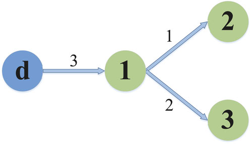
FIGURE 2. Topology of communication graph.

It can be easily obtained from Figure 2 that $A=\left[\begin{array}{ccc}\hfill 0\hfill & \hfill 0\hfill & \hfill 0\hfill \\ \hfill 1\hfill & \hfill 0\hfill & \hfill 0\hfill \\ \hfill 2\hfill & \hfill 0\hfill & \hfill 0\hfill \end{array}\right]$ represents the adjacency matrix, $D=\left[\begin{array}{ccc}\hfill 0\hfill & \hfill 0\hfill & \hfill 0\hfill \\ \hfill 0\hfill & \hfill 1\hfill & \hfill 0\hfill \\ \hfill 0\hfill & \hfill 0\hfill & \hfill 2\hfill \end{array}\right]$ is the in-degree matrix, and $L=\left[\begin{array}{ccc}\hfill 0\hfill & \hfill 0\hfill & \hfill 0\hfill \\ \hfill -1\hfill & \hfill 1\hfill & \hfill 0\hfill \\ \hfill -2\hfill & \hfill 0\hfill & \hfill 2\hfill \end{array}\right]$ indicates the Laplacian matrix. In addition, we can obtain that d₁ = 0, d₂ = 1, d₃ = 2, b₁ = 3, b₂ = 0, and b₃ = 0.

In the simulation, we choose the parameters of system (1) as J₁ = 0.02 Kgm², J₂ = 0.16 Kgm², F₁ = 1.4Nms/rad, F₂ = 2.5Nms/rad, K = 10, K_t = 10Nm/A, K_b = 0.1Nm/A, N = 0.09, M = 1Kg, g = 10N/Kg, d = 0.06m, L = 10H, and R = 0.05Ω. Next, the desired signal is selected as y_d = −15 cos t.

The incipient conditions are $x_1(0)={\left[0.5,\mathrm{0,0.1},0.1,0.1\right]}^T$, $x_2(0)={\left[0.5,\mathrm{0,0.1},0.1,0.1\right]}^T$, and $x_3(0)={\left[0.5,\mathrm{0,0.1},0.1,0.1\right]}^T$. The design parameters are chosen as c_1,1 = 40, c_1,2 = 0.05, c_1,3 = 0.1, c_1,4 = c_1,5 = 0.001, c_2,1 = 49, c_2,2 = 1, c_2,3 = 0.1, c_2,4 = 0.05, c_2,5 = 0.1, c_3,1 = 44, c_3,2 = 1.4, c_3,3 = 0.02, c_3,4 = c_3,5 = 0.1, e_1,1 = 0.0001, e_1,2 = e_1,3 = 0.0008, e_1,4 = e_1,5 = 0.001, e_2,1 = 0.0001, e_2,2 = e_2,3 = 0.0008, e_2,4 = e_2,5 = 0.001, e_3,1 = 0.0001, e_3,2 = e_3,3 = 0.0008, e_3,4 = 0.001, e_3,5 = 0.0008, λ_1,1 = 0.015, λ_1,2 = 0.002, λ_1,3 = λ_1,4 = 0.01, λ_1,5 = 0.008, λ_2,1 = 0.01, λ_2,2 = 0.002, λ_2,3 = λ_2,4 = 0.01, λ_2,5 = 0.008, λ_3,1 = 0.01, λ_3,2 = 0.001, λ_3,3 = λ_3,4 = 0.01, λ_3,5 = 0.008, a_1,1 = 2, a_1,2 = a_1,4 = 50, a_1,5 = 200, a_2,1 = 3, a_2,2 = a_2,4 = 50, a_2,5 = 20, a_3,1 = 2, a_3,2 = a_3,4 = 50, a_3,5 = 20, τ_1,1 = 0.7, τ_1,2 = 700, τ_1,4 = 1, τ_1,5 = 0.2, τ_2,1 = 50, τ_2,2 = 20, τ_2,4 = 0.5, τ_2,5 = 50, τ_3,1 = 30, τ_3,2 = 20, τ_3,4 = 0.25, τ_3,5 = 50, σ_1,1 = 150, σ_1,2 = 200, σ_1,4 = 10, σ_1,5 = 400, σ_2,1 = 10, σ_2,2 = 1, σ_2,4 = 10, σ_2,5 = 1, σ_3,1 = 10, σ_3,2 = 1, σ_3,4 = 11, σ_3,5 = 1, r_i,j = 10(i = 1, 2, 3; j = 1, 2, 4, 5), and p = 81/101.

The simulation results are displayed in Figures 3–8. Figure 3 displays the output trajectories of three followers and the leader. Figure 4 indicates the consensus tracking errors of three followers, which obviously converge to a small neighborhood of origin within a finite time. Figures 5–8 display the trajectories of the adaptive laws, which show that these signals are bounded. According to the simulation results, we know that all the signals in the closed-loop systems remain bounded.

FIGURE 3

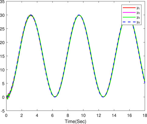
FIGURE 3. The output trajectories of three followers and the leader.

FIGURE 4

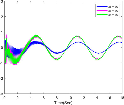
FIGURE 4. The consensus tracking errors of three followers.

FIGURE 5

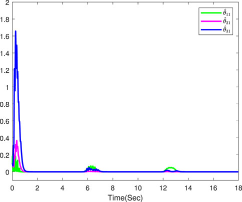
FIGURE 5. The first adaptive law of three followers.

FIGURE 6

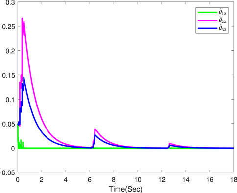
FIGURE 6. The second adaptive law of three followers.

FIGURE 7

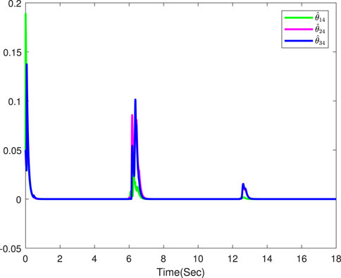
FIGURE 7. The third adaptive law of three followers.

FIGURE 8

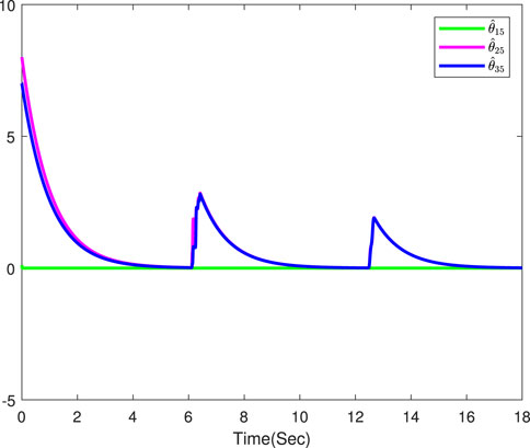
FIGURE 8. The fourth adaptive law of three followers.

5 Conclusion

This article has proposed an adaptive command-filtered finite-time consensus control strategy for the considered single-link flexible-joint robotic MASs. First, RBF NN technology was used to approximate the unknown nonlinearities in the system, so the design challenges due to the unknown nonlinearities have been solved. Second, the problem of “explosion of complexity” in the backstepping process has been successfully settled by using the command filtering technology with the new compensation signals, which eliminated the error impact posed by the command filters. It is seen that the presented adaptive command-filtered finite-time consensus control strategy ensured that the tracking errors converge to a small neighborhood of origin within a finite time, and all signals in the closed-loop systems are bounded. Eventually, the validity of the proposed control scheme has been proven by the simulation example. Next, we will research the consensus tracking control with the fixed-time and the predefined-time for the studied single-link flexible-joint robotic MASs.

Data availability statement

The original contributions presented in the study are included in the article/Supplementary Material; further inquiries can be directed to the corresponding author.

Author contributions

CL, LH, BY, BN, SL, and XL contributed the idea and design of the study. CL wrote the first draft of the manuscript. CL organized the literature. LH, BY, and BN performed the design of figures. SL and XL verified the experimental design. All authors contributed to the article and approved the submitted version.

Conflict of interest

The authors declare that the research was conducted in the absence of any commercial or financial relationships that could be construed as a potential conflict of interest.

Publisher’s note

All claims expressed in this article are solely those of the authors and do not necessarily represent those of their affiliated organizations, or those of the publisher, the editors, and the reviewers. Any product that may be evaluated in this article, or claim that may be made by its manufacturer, is not guaranteed or endorsed by the publisher.

References

1. Diao S, Sun W, Su S-F. Neural-based adaptive event-triggered tracking control for flexible-joint robots with random noises. Int J Robust Nonlinear Control (2022) 32:2722–40. doi:10.1002/rnc.5382

CrossRef Full Text | Google Scholar

2. Yin S, Shi P, Yang H. Adaptive fuzzy control of strict-feedback nonlinear time-delay systems with unmodeled dynamics. IEEE Trans cybernetics (2015) 46:1926–38. doi:10.1109/tcyb.2015.2457894

CrossRef Full Text | Google Scholar

3. Ma H, Zhou Q, Li H, Lu R. Adaptive prescribed performance control of a flexible-joint robotic manipulator with dynamic uncertainties. IEEE Trans Cybernetics (2021) 52:12905–15. doi:10.1109/tcyb.2021.3091531

CrossRef Full Text | Google Scholar

4. Ding S, Peng J, Zhang H, Wang Y. Neural network-based adaptive hybrid impedance control for electrically driven flexible-joint robotic manipulators with input saturation. Neurocomputing (2021) 458:99–111. doi:10.1016/j.neucom.2021.05.095

CrossRef Full Text | Google Scholar

5. Zaare S, Soltanpour MR, Moattari M Voltage based sliding mode control of flexible joint robot manipulators in presence of uncertainties. Robotics Autonomous Syst (2019) 118:204–19. doi:10.1016/j.robot.2019.05.014

CrossRef Full Text | Google Scholar

6. Zaare S, Soltanpour MR, Moattari M. Adaptive sliding mode control of $n$ flexible-joint robot manipulators in the presence of structured and unstructured uncertainties. Multibody Syst Dyn (2019) 47:397–434. doi:10.1007/s11044-019-09693-1

CrossRef Full Text | Google Scholar

7. Liu L, Yao W, Guo Y. Prescribed performance tracking control of a free-flying flexible-joint space robot with disturbances under input saturation. J Franklin Inst (2021) 358:4571–601. doi:10.1016/j.jfranklin.2021.03.001

CrossRef Full Text | Google Scholar

8. Kim J, Croft EA. Full-state tracking control for flexible joint robots with singular perturbation techniques. IEEE Trans Control Syst Tech (2017) 27:63–73. doi:10.1109/tcst.2017.2756962

CrossRef Full Text | Google Scholar

9. Chen C, Lewis FL, Li X. Event-triggered coordination of multi-agent systems via a lyapunov-based approach for leaderless consensus. Automatica (2022) 136:109936. doi:10.1016/j.automatica.2021.109936

CrossRef Full Text | Google Scholar

10. Liu J, Zhang Y, Yu Y, Sun C. Fixed-time leader–follower consensus of networked nonlinear systems via event/self-triggered control. IEEE Trans Neural networks Learn Syst (2020) 31:5029–37. doi:10.1109/tnnls.2019.2957069

CrossRef Full Text | Google Scholar

11. Li H, Liu Q, Feng G, Zhang X. Leader–follower consensus of nonlinear time-delay multiagent systems: A time-varying gain approach. Automatica (2021) 126:109444. doi:10.1016/j.automatica.2020.109444

CrossRef Full Text | Google Scholar

12. Zhang J, Zhang H, Sun S, Gao Z. Leader-follower consensus control for linear multi-agent systems by fully distributed edge-event-triggered adaptive strategies. Inf Sci (2021) 555:314–38. doi:10.1016/j.ins.2020.10.056

CrossRef Full Text | Google Scholar

13. Li Y-X. Barrier lyapunov function-based adaptive asymptotic tracking of nonlinear systems with unknown virtual control coefficients. Automatica (2020) 121:109181. doi:10.1016/j.automatica.2020.109181

CrossRef Full Text | Google Scholar

14. Niu B, Zhao P, Liu J-D, Ma H-J, Liu Y-J. Global adaptive control of switched uncertain nonlinear systems: An improved mdadt method. Automatica (2020) 115:108872. doi:10.1016/j.automatica.2020.108872

CrossRef Full Text | Google Scholar

15. Niu B, Liu J, Wang D, Zhao X, Wang H. Adaptive decentralized asymptotic tracking control for large-scale nonlinear systems with unknown strong interconnections. IEEE/CAA J Automatica Sinica (2021) 9:173–86. doi:10.1109/jas.2021.1004246

CrossRef Full Text | Google Scholar

16. Niu B, Kong J, Zhao X, Zhang J, Wang Z, Li Y. Event-triggered adaptive output-feedback control of switched stochastic nonlinear systems with actuator failures: A modified mdadt method. IEEE Trans Cybernetics (2022) 53:900–12. doi:10.1109/tcyb.2022.3169142

CrossRef Full Text | Google Scholar

17. Niu B, Zhang Y, Zhao X, Wang H, Sun W. Adaptive predefined-time bipartite consensus tracking control of constrained nonlinear mass: An improved nonlinear mapping function method. IEEE Trans Cybernetics (2023) 1–10. doi:10.1109/tcyb.2022.3231900

CrossRef Full Text | Google Scholar

18. Niu B, Chen W, Su W, Wang H, Wang D, Zhao X. Switching event-triggered adaptive resilient dynamic surface control for stochastic nonlinear cpss with unknown deception attacks. IEEE Trans Cybernetics (2022) 1–9. doi:10.1109/tcyb.2022.3209694

CrossRef Full Text | Google Scholar

19. Tang F, Niu B, Wang H, Zhang L, Zhao X. Adaptive fuzzy tracking control of switched mimo nonlinear systems with full state constraints and unknown control directions. IEEE Trans Circuits Syst Express Briefs (2022) 69:2912–6. doi:10.1109/tcsii.2022.3149886

CrossRef Full Text | Google Scholar

20. Zhang L, Che W-W, Chen B, Lin C. Adaptive fuzzy output-feedback consensus tracking control of nonlinear multiagent systems in prescribed performance. IEEE Trans Cybernetics (2022) 53:1932–43. doi:10.1109/tcyb.2022.3171239

CrossRef Full Text | Google Scholar

21. Chen M, Wang H, Liu X. Adaptive fuzzy practical fixed-time tracking control of nonlinear systems. IEEE Trans Fuzzy Syst (2019) 29:664–73. doi:10.1109/tfuzz.2019.2959972

CrossRef Full Text | Google Scholar

22. Li Y-X, Hu X, Che W, Hou Z. Event-based adaptive fuzzy asymptotic tracking control of uncertain nonlinear systems. IEEE Trans Fuzzy Syst (2020) 29:3003–13. doi:10.1109/tfuzz.2020.3010643

CrossRef Full Text | Google Scholar

23. Li Y, Shao X, Tong S. Adaptive fuzzy prescribed performance control of nontriangular structure nonlinear systems. IEEE Trans Fuzzy Syst (2019) 28:2416–26. doi:10.1109/tfuzz.2019.2937046

CrossRef Full Text | Google Scholar

24. Yu X, He W, Li H, Sun J. Adaptive fuzzy full-state and output-feedback control for uncertain robots with output constraint. IEEE Trans Syst Man, Cybernetics: Syst (2020) 51:6994–7007. doi:10.1109/tsmc.2019.2963072

CrossRef Full Text | Google Scholar

25. Yilmaz BM, Tatlicioglu E, Savran A, Alci M. Adaptive fuzzy logic with self-tuned membership functions based repetitive learning control of robotic manipulators. Appl Soft Comput (2021) 104:107183. doi:10.1016/j.asoc.2021.107183

CrossRef Full Text | Google Scholar

26. Fuentes-Aguilar RQ, Chairez I. Adaptive tracking control of state constraint systems based on differential neural networks: A barrier lyapunov function approach. IEEE Trans Neural networks Learn Syst (2020) 31:5390–401. doi:10.1109/tnnls.2020.2966914

CrossRef Full Text | Google Scholar

27. Wu L-B, Park JH, Xie X-P, Liu Y-J. Neural network adaptive tracking control of uncertain mimo nonlinear systems with output constraints and event-triggered inputs. IEEE Trans Neural networks Learn Syst (2020) 32:695–707. doi:10.1109/tnnls.2020.2979174

CrossRef Full Text | Google Scholar

28. Liu Y-J, Zhao W, Liu L, Li D, Tong S, Chen CP. Adaptive neural network control for a class of nonlinear systems with function constraints on states. IEEE Trans Neural Networks Learn Syst (2021) 34 1–10. doi:10.1109/tnnls.2021.3107600

CrossRef Full Text | Google Scholar

29. Liu P, Yu H, Cang S. Adaptive neural network tracking control for underactuated systems with matched and mismatched disturbances. Nonlinear Dyn (2019) 98:1447–64. doi:10.1007/s11071-019-05170-8

CrossRef Full Text | Google Scholar

30. Feng Y, Zheng WX. Adaptive tracking control for nonlinear heterogeneous multi-agent systems with unknown dynamics. J Franklin Inst (2019) 356:2780–97. doi:10.1016/j.jfranklin.2018.12.003

CrossRef Full Text | Google Scholar

31. Sun Y, Chen B, Lin C, Wang H. Adaptive neural control for a class of stochastic non-strict-feedback nonlinear systems with time-delay. Neurocomputing (2016) 214:750–7. doi:10.1016/j.neucom.2016.06.060

CrossRef Full Text | Google Scholar

32. Swaroop D, Hedrick JK, Yip PP, Gerdes JC. Dynamic surface control for a class of nonlinear systems. IEEE Trans automatic Control (2000) 45:1893–9. doi:10.1109/tac.2000.880994

CrossRef Full Text | Google Scholar

33. Shi X, Cheng Y, Yin C, Huang X, Zhong S-M. Design of adaptive backstepping dynamic surface control method with rbf neural network for uncertain nonlinear system. Neurocomputing (2019) 330:490–503. doi:10.1016/j.neucom.2018.11.029

CrossRef Full Text | Google Scholar

34. von Ellenrieder KD. Dynamic surface control of trajectory tracking marine vehicles with actuator magnitude and rate limits. Automatica (2019) 105:433–42. doi:10.1016/j.automatica.2019.04.018

CrossRef Full Text | Google Scholar

35. Zhang J, Li S, Ahn CK, Xiang Z. Adaptive fuzzy decentralized dynamic surface control for switched large-scale nonlinear systems with full-state constraints. IEEE Trans Cybernetics (2021) 52:10761–72. doi:10.1109/tcyb.2021.3069461

CrossRef Full Text | Google Scholar

36. Chen Z, Niu B, Zhang L, Zhao J, Ahmad AM, Alassafi MO. Command filtering-based adaptive neural network control for uncertain switched nonlinear systems using event-triggered communication. Int J Robust Nonlinear Control (2022) 32:6507–22. doi:10.1002/rnc.6154

CrossRef Full Text | Google Scholar

37. Bhat SP, Bernstein DS. Finite-time stability of continuous autonomous systems. SIAM J Control optimization (2000) 38:751–66. doi:10.1137/s0363012997321358

CrossRef Full Text | Google Scholar

38. Li H, Zhao S, He W, Lu R. Adaptive finite-time tracking control of full state constrained nonlinear systems with dead-zone. Automatica (2019) 100:99–107. doi:10.1016/j.automatica.2018.10.030

CrossRef Full Text | Google Scholar

39. Wang F, Liu Z, Li X, Zhang Y, Chen CP. Observer-based finite time control of nonlinear systems with actuator failures. Inf Sci (2019) 500:1–14. doi:10.1016/j.ins.2019.05.067

CrossRef Full Text | Google Scholar

40. Yu J, Zhao L, Yu H, Lin C, Dong W. Fuzzy finite-time command filtered control of nonlinear systems with input saturation. IEEE Trans cybernetics (2017) 48:2378–87. doi:10.1109/TCYB.2017.2738648

CrossRef Full Text | Google Scholar

41. Diao S, Sun W, Su S-F, Xia J. Adaptive fuzzy event-triggered control for single-link flexible-joint robots with actuator failures. IEEE Trans Cybernetics (2021) 52:7231–41. doi:10.1109/tcyb.2021.3049536

CrossRef Full Text | Google Scholar

42. Ma C, Wu W. Distributed leader-follower consensus of nonlinear multi-agent systems with unconsensusable switching topologies and its application to flexible-joint manipulators. Syst Sci Control Eng (2018) 6:200–7. doi:10.1080/21642583.2018.1547991

CrossRef Full Text | Google Scholar

43. Polycarpou MM, Ioannou PA. A robust adaptive nonlinear control design. In: 1993 American control conference; June 2-4, 1993; San Francisco. IEEE (1993). p. 1365–9.

CrossRef Full Text | Google Scholar

44. Farrell JA, Polycarpou M, Sharma M, Dong W. Command filtered backstepping. IEEE Trans Automatic Control (2009) 54:1391–5. doi:10.1109/tac.2009.2015562

CrossRef Full Text | Google Scholar

45. Wang F, Chen B, Liu X, Lin C. Finite-time adaptive fuzzy tracking control design for nonlinear systems. IEEE Trans Fuzzy Syst (2017) 26:1207–16. doi:10.1109/tfuzz.2017.2717804

CrossRef Full Text | Google Scholar

46. Li Y-X. Finite time command filtered adaptive fault tolerant control for a class of uncertain nonlinear systems. Automatica (2019) 106:117–23. doi:10.1016/j.automatica.2019.04.022

CrossRef Full Text | Google Scholar

47. Shang Y, Chen B, Lin C. Consensus tracking control for distributed nonlinear multiagent systems via adaptive neural backstepping approach. IEEE Trans Syst Man, Cybernetics: Syst (2018) 50:2436–44. doi:10.1109/tsmc.2018.2816928

CrossRef Full Text | Google Scholar

48. Huang X, Lin W, Yang B. Global finite-time stabilization of a class of uncertain nonlinear systems. Automatica (2005) 41:881–8. doi:10.1016/j.automatica.2004.11.036

CrossRef Full Text | Google Scholar